Test of OPE and OGE through mixing angles of negative parity
$N^{*}$ resonances in electromagnetic transitions

Abstract

In this report, by using the mixing angles of one-gluon-exchange model(OGE) and one-pion-exchange model(OPE), and by using the electromagnetic Hamiltonian of Close and Li, we calculate the amplitudes of $L=1$ $N^{*}$ resonances for photoproduction and electroproduction. The results are compared to experimental data. It’s found that the data support OGE, not OPE.

Which is the interaction between quarks mediated by, glouns or mesons? In one form or another, it has been used in a wide variety of models for the last two decades. In 2000, Isgur published his critiquecritique to the reviewGR of Glozman and Riska in which it is proposed that baryon spectroscopy can be described by OPE without the standard OGE forces of ref. IK and OGE .

In the critique, it is said that predicting the spectrum of baryon resonances is not a very stringent test of a model. A prototypical example is properties of the two $N^{*}_{1/2^{-}}$ states. Among models which perfectly describe the spectrum, there is still a composition of these states since all values of $\theta_{{1/2}^{-}}$ from 0 to $\pi$ correspond to distinct states. OPE model predicts $\theta_{1/2^{-}}=\pm 13^{\circ}$ and $\theta_{3/2^{-}}=\pm 8^{\circ}$. Such a $\theta_{1/2^{-}}$ has almost no impact on explaining the anomalously large N$\eta$ branching ratio of the $N^{*}(1535)_{1/2^{-}}$ and the anomalously small N$\eta$ branching ratio of the $N^{*}(1650)_{1/2^{-}}$.

Recently, by using the method of Isgur and Karl IK77 , Chizma and Karl gave another values of mixing angles of OPE, $\theta_{1/2^{-}}=25.5^{\circ}$ and $\theta_{3/2^{-}}=-52.7^{\circ}$ CK . Their results are independent of spectrum and decay data. We know that most values of mixing angles including the ”experiment” one are obtained through fitting the spectrum and decay. The error of ”experiment” values of Hey $et.al.$ expangle is of order of $10^{\circ}$. Thus, we can’t judge which model is better through only comparing with ”experiment” mixing angle values. Since the predicting of the spectrum of states is not enough to test a model critique , it is necessary to examine the exchange models with further experimental data. Here, we will compare OPE and OGE in eletroproduction and photoproduction through the mixing angles. Using the wave functions obtained by Chizma and Karl, we calculate the amplitudes of transition from ground state to $L=1$ $N^{*}$ resonances, then compare results with experiment to test different models.

In ref. CK , Chizma and Karl used the OGE and OPE interaction Hamiltonians as following:

$$H_{hyp}^{OGE}= A\{(8\pi/3)\ {\bf S}_{1}\cdot{\bf S}_{2}\ \ \delta^{3}({\bf\rho})\ \ \ \$$ (1)

$$+(3{\bf S}_{1}\cdot\widehat{{\bf\rho}}\ {\bf S}_{2}\cdot\widehat{{\bf\rho}}-{\bf S}_{1}\cdot{\bf S}_{2})\ \rho^{-3}\}\ ,$$

$$H_{hyp}^{OPE}= B\{(-4\pi/3)\ {\bf S}_{1}\cdot{\bf S}_{2}\ \ \delta^{3}({\bf\rho})$$ (2)

$$+(3{\bf S}_{1}\cdot\widehat{{\bf\rho}}\ {\bf S}_{2}\cdot\widehat{{\bf\rho}}-{\bf S}_{1}\cdot{\bf S}_{2})\ \rho^{-3}\}\ {\bf\lambda}_{1}^{f}\cdot{\bf\lambda}_{2}^{f}\ ,$$

where, $\hat{\rho}=\frac{\overrightarrow{\rho}}{|\overrightarrow{\rho}|}$. A, or B, is an overall constant which determines the strength of the interaction. ${\bf S}_{1,2}$, $\lambda^{f}_{1,2}$ are spins and the eight $3\times 3$ Gell-Mann SU(3) flavor matrices for quarks number 1 and 2. Here we assumed the mass of pion is zero because it does not change the results significantly.

Ignoring the color wavefunction, the harmonic-oscillator wavefunctions for $L=1$ $N^{*}$ resonances have following forms:IK

$$S=3/2: \Psi(^{4}P)=\frac{1}{\sqrt{2}}\chi^{s}\{\psi^{\lambda}\phi^{\lambda}+\psi^{\rho}\phi^{\rho}\}\ ,$$ (3)

$$S=1/2: \Psi(^{2}P)=\frac{1}{2}\{\chi^{\lambda}\psi^{\rho}\phi^{\rho}+\chi^{\rho}\psi^{\lambda}\phi^{\rho}+\chi^{\rho}\psi^{\rho}\phi^{\lambda}$$ (4)

$$-\chi^{\lambda}\psi^{\lambda}\phi^{\lambda}\}\ .$$

The spin angular momentum $S=1/2$ or $3/2$ has to be coupled with the orbital angular momentum $L=1$ to give the total angular momentum $|L+S|\geq J\geq|L-S|$. As a result there are two states each at $J=1/2$ and $J=3/2$, namely spin doublet and spin quartet: ${}^{2}P_{1/2}$,${}^{4}P_{1/2}$ and ${}^{2}P_{3/2}$,${}^{4}P_{3/2}$. The physical eigenstates are linear combinations of these two states, and can be obtained by diagonalizing the Hamiltonian in this space of states. Then, mixing angles are : CK

$$OPE:\ \theta_{3/2}=-52.7^{\circ},\ \theta_{1/2}=25.5^{\circ}\ ;$$

$$OGE:\ \theta_{3/2}=6^{\circ},\ \theta_{1/2}=-32^{\circ}\ ,$$ (5)

and the wave functions have the forms:

$$|N1700\rangle=cos\theta_{3/2}|^{4}P_{3/2}\rangle+sin\theta_{3/2}|^{2}P_{3/2}\rangle\ ,$$

$$|N1520\rangle=-sin\theta_{3/2}|^{4}P_{3/2}\rangle+cos\theta_{3/2}|^{2}P_{3/2}\rangle\ ,$$ (6)

$$|N1650\rangle=cos\theta_{1/2}|^{4}P_{1/2}\rangle+sin\theta_{1/2}|^{2}P_{1/2}\rangle\ ,$$

$$|N1535\rangle=-sin\theta_{1/2}|^{4}P_{1/2}\rangle+cos\theta_{1/2}|^{2}P_{1/2}\rangle\ .$$ (7)

To calculate the electromagnetic transition amplitudes, we use the electromagnetic interaction of Close and Li CL which can be derived from B-S equation brodsky . It avoids the explicit appearance of the binding potential through the method of McClary and Byers MB . Its explicit form is:

$$H^{em} = \sum_{i=1}^{3}H_{i}=\sum_{i=1}^{3}\{-e_{i}{\bf r}_{i}\cdot{\bf E}_{i}+i\frac{e_{i}}{2m^{*}}({\bf p}_{i}\cdot{\bf k}_{i}{\bf r}_{i}\cdot{\bf A}_{i}+{\bf r}_{i}\cdot{\bf A}_{i}{\bf p}_{i}\cdot{\bf k}_{i})-\mu_{i}{\bf\sigma}_{i}{\bf B}_{i}$$ (8)

$$-\frac{1}{2m^{*}}(2\mu_{i}-\frac{e_{i}}{2m^{*}})\frac{{\bf\sigma}_{i}}{2}\cdot[{\bf E}_{i}\times{\bf p}_{i}-{\bf p}_{i}\times{\bf E}_{i}]\}+\sum_{i<j}\frac{1}{2M_{T}m^{*}}(\frac{{\bf\sigma}_{i}}{2}-\frac{{\bf\sigma}_{j}}{2})\cdot[e_{j}{\bf E}_{j}\times{\bf p}_{i}-e_{i}{\bf E}_{i}\times{\bf p}_{i}]\ ,$$

where we keep to O $(1/m^{2})$, and use long wave approximation. ${\bf E}_{i}$ and ${\bf B}_{i}$ are the electromagnetic fields, $e_{i}$, ${\bf\sigma}_{i}$, $\mu_{i}$ are the charge, spin, and magnetic moment of quark $i$. $M_{T}$ is recoil mass. $m^{*}_{i}$ is the effective quark mass including the effect of long-range scalar simple harmonic potential, but it is independent on the exchange potential. So $\mu_{i}$ or $m_{i}^{*}$ in two models can be treated as the same free parameters.

By insertion of the usual radiation field for the absorption of a photon into Eq.(8), and by integrating over the baryon center-of-mass coordinate, we obtain the transverse photoexcited value over flavor spin and spatial coordinates C

$$A_{\lambda}^{N}=\sum_{i=1}^{3}\langle X;J\lambda|H_{i}|N;\frac{1}{2}\lambda-1\rangle\ .$$ (9)

Here the initial photon has a momentum $\mathbf{k}||\widehat{z}$. A simple procedure, that of transforming the wave functions to a basis which has redefined Jacobi coordinates, allows the calculation of the matrix elements of the $H_{1}$ and $H_{2}$ operators to proceed in an exactly similar way to that of the operator $H_{3}$. Calculation of the matrix elements of $H_{3}$ avoids complicated functions of the relative coordinates in the ”recoil” exponential.

By using the wave functions (6), (7), or non-admixture wave functions (which can be seen as the wave functions with zero mixing angles ) and by using Hamiltonian (8), we calculate the amplitudes of photoexitation from the ground states N(p,n) to the resonance X by Eq. (9) in Breit-frame. In the calculation, we follow the convention of Koniuk and Isgur KI . For the photocouplings of the states made of light quarks, and the states which are not highly exited, it should be a reasonable approximation to treat the quark kinetic mass $m^{*}_{i}$ as a constant effective mass $m^{*}$. As the reference C , We keep recoil mass at $M_{T}=3m^{*}$, and use parameter values, $\alpha=0.5GeV$, and $m^{*}=0.437GeV$. (in fact, the result isn’t sensitive to the values of $M_{T}$ and $m^{*}$)

In the photoproduction, nucleon is excited by a real photon, which mass equals to zero, $i.e.$ $Q^{2}=0$ (here $Q^{2}=-q^{2}$,where $q^{\mu}$ is the transferred four-momentum). A useful measure of the quality of the fit is to form a $\chi^{2}$ statistic in the usual way. Introducing a ”theoretical error” error avoids overemphasis in the fitting procedure of a few very well-measured photocouplings. In Table I, we give amplitudes and $\chi^{2}$ of non-admixture, of OPE, and of OGE, and list the experimental values in last column.

Table 1: Breit-frame photoproduction amplitudes using wave function of no-admixture(NA), of OPE, and of OGE. Here $\alpha=0.5GeV$, $m^{*}=0.437GeV$, g=1.3, $M_{T}=3m^{*}$. Amplitudes are in units of $10^{-3}Gev^{1/2}$; a factor of +i is suppressed for all amplitudes. Experimental values are from PDG PDG

state	$A_{\lambda}^{N}$	NA	$\chi^{2}_{NA}$	OPE	$\chi^{2}_{OPE}$	OGE	$\chi^{2}_{OGE}$	Expt.
$N\frac{3}{2}^{-}(1700)$	$A^{p}_{\frac{1}{2}}$	-21	0.0	29	3.9	-26	0.1	$-18\pm 13$
	$A^{n}_{\frac{1}{2}}$	19	0.1	33	0.4	17	0.1	$0\pm 50$
	$A^{p}_{\frac{3}{2}}$	-36	1.3	-131	17.2	-21	0.4	$-1\pm 24$
	$A^{n}_{\frac{3}{2}}$	-14	0.1	89	3.6	-27	0.2	$-3\pm 44$
$N\frac{3}{2}^{-}(1520)$	$A^{p}_{\frac{1}{2}}$	-23	0.0	-31	0.1	-21	0.0	$-24\pm 9\$
	$A^{n}_{\frac{1}{2}}$	-38	1.0	-5	6.2	-40	0.8	$-59\pm 9\$
	$A^{p}_{\frac{3}{2}}$	139	1.8	55	29.0	142	1.4	$166\pm 5\$
	$A^{n}_{\frac{3}{2}}$	-125	0.4	-74	8.1	-124	0.4	$-139\pm 11$
$N\frac{1}{2}^{-}(1650)$	$A^{p}_{\frac{1}{2}}$	19	1.8	-35	11.9	81	1.2	$53\pm 16$
	$A^{n}_{\frac{1}{2}}$	-1	0.2	36	3.1	-46	1.1	$-15\pm 21$
$N\frac{1}{2}^{-}(1535)$	$A^{p}_{\frac{1}{2}}$	109	0.3	106	0.2	82	0.0	$90\pm 30$
	$A^{n}_{\frac{1}{2}}$	-82	1.1	-75	0.8	-66	0.4	$-46\pm 27$

In the first two columns of Table I, the amplitudes without admixture and $\chi^{2}$ of those amplitudes are displayed. We can see that amplitudes of many states agree with experimental data well. But $A_{1/2}^{p}$ for $N(1650)$, $A_{3/2}^{p}$ for $N(1520)$, $A_{1/2}^{n}$ for $N(1535)$ and $A_{3/2}^{p}$ for $N(1700)$ should be uplifted. $A_{3/2}^{n}$ for $N(1520)$ and $A_{1/2}^{n}$ for $N(1520)$ should be suppressed. Obviously, if we mix two spin-1/2 states and spin-3/2 states separately as Equs. [6], and [7], we can realize it. The other noteworthy information we can get from the first two columns is that the difference between $A_{1/2}^{p,n}$ for $N(1650)$ and $A_{1/2}^{p,n}$ for $N(1535)$, or the difference between $A_{3/2}^{p,n}$ for $N(1700)$ and $A_{3/2}^{p,n}$ for $N(1520)$, is too large. So the admixture should not be very large. Otherwise the results which have agreed with experiment will be destroyed. The third and forth columns in Table I give the results of OPE. Except $A_{1/2}^{p,n}$ for $N(1535)$, $\chi^{2}$ of most amplitudes increase. $\chi^{2}$ of $A_{1/2}^{p}$ for $N(1650)$, $A_{3/2}^{p}$ for $N(1700)$, or $A_{3/2}^{p}$ for $N(1520)$, is even larger than 10. All those amplitudes are obtained by mixing two amplitudes with large difference. Even some states change to wrong direction. For example, $A_{1/2}^{p}$ for $N(1650)$ should be uplifted, but admixture of OPE makes it lower. The sum $\chi^{2}$ of twelve amplitudes also increases from 8.0 to 84.6. The fifth and sixth columns present results of OGE. Admixture of OGE gives significant improvement on no-admixture results. Almost all amplitudes agree with experiment well. The sum value of $\chi^{2}$ decreases from 8.0 to 6.2.

Electroproduction amplitudes are extracted from eN scattering. In this procedure, nucleon is excited from ground state to excited state by a virtual photon, which mass isn’t zero, $i.\ e.$ $-Q^{2}\neq 0$. In Fig 1, We draw curves of calculated amplitudes, which vary with $Q^{2}$. The results of no-admixture, OPE, and OGE are presented along with experimental data in the figure.

In Fig. 1 (b), $A_{1/2}^{p}$ for $N(1535)$, and Fig. 1 (d), $A_{1/2}^{p}$ for $N(1520)$, the differences between OPE and OGE are small. The relativistic effect on wave functions, which we did not consider in this paper, may smear the small differences. So they are useless to compare OPE and OGE. Discrepancies of different models in the other two graphs are large. In Fig 1 (a), $A_{1/2}^{p}$ for $N(1650)$, and (c), $A_{3/2}^{p}$ for $N(1520)$, OGE is superior to OPE obviously. In addition, we can see that in Fig. 1 (a) the curve without admixture is between those of OPE and OPE. It suggest that one of models will give wrong direction correction. According to data and our results of photoproduction, it should be OPE. In Fig. 1 (c) OPE gives too large correction obviously.

Though we use the non-relativistic wave functions here, from Table I of reference C and from the calculations of this paper, we can find that relativistic effect won’t reverse our conclusion. For the most results with large differences between OPE and OGE, the conclusion can be kept when we change mixing angles of OPE and OGE separately by $\pm 10^{\circ}$. For example, the sum of $\chi^{2}$ for OGE varies between 5.1 and 11.3, and that of OPE varies between 57.5 and 117.5. In this case, OGE is still superior to OPE obviously. Through our calculation, it is believable that the OGE is better than OPE in fit with photoproduction and electroproduction amplitudes of the $N^{*}$ resonances with negative parity. In other words, OGE gives consistent mixing angles to explain spectrum, decay branching, photoproduction and electroproduction amplitudes.

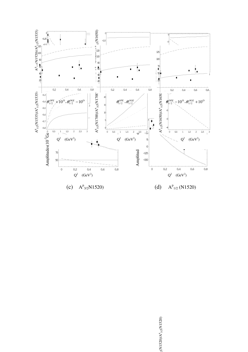
Figure 1: Breit-frame electroproduction amplitudes. Here $\alpha=0.5GeV$, $m^{*}=0.437GeV$, g=1.3, $M_{T}=3m^{*}$. A factor of +i is suppressed. Full curves are calculated in OGE, dashed ones in OPE, and dotted ones without admixture. Experimental values are from WSWR ; data ; PDG

- (1) N. Isgur, Phys.Rev.D 62, 054026(2000).
- (2) L. Ya Glozman and D. O. Riska, Phys. Rep. 268, 263(1996); L. Y. Glozman, nul-th/9909021.
- (3) N. Isgur and G. Karl, Phys. Lett. B72, 109(1977); Phys. Lett. B74,353(1978); Phys. Rev. D18, 4187(1978); Phys. Rev. 2653(1979).
- (4) A. De Rjula, H. Georgi, S. L. Glashow, Phys. Rev. D12, 147(1975).
- (5) N. Isgur and G. Karl, Phys. Lett. B72, 109(1977).
- (6) J. Chizma and G. Karl, hep-ph/0210126. According to private communication, there is a mistake in this article: B is positive indeed. Then correct values of mixing angles are given in eq.(5).
- (7) A. J. G. Hey, P. J. Litchfield and R. J. Cashmore, Nucl. Phys. B95, 516(1975).
- (8) Frank E. Close and Zhenping Li, Phys. Rev. D42, 2194(1990).
- (9) S. J. Brodsky and J. Primack, Ann. Phys. (N.Y.1) 52, 315 (1969).
- (10) Richard McClary and Nina Byers, Phys. Rev. D28 1692(1983).
- (11) Simon Capstick, Phy. Rev. D46, 2864(1992).
- (12) Roman Koniuk and Nathan Isgur, Phys. Rev. D21, 1868(1980).
- (13) Particle Data Group, J. J. Hernndez , Phys. Lett. B239, 1(1990).
- (14) Particle Data Group, Phys. Rev. D66 1-I(2002).
- (15) M. Warns, H. Schröder, W. Pfeil and H. Rollnik, Z. Phy. C45, 627(1990).
- (16) V.D. Burkert, R. De Vita, M. Battaglieri, M. Ripani and V. Mokeev, JLAB-PHY-02-23, Dec 2002. e-Print Archive: hep-ph/0212108.