Relativistic formulation of Glauber theory for $A(e,e^{\prime}p)$ reactions

Abstract

At sufficiently large proton energies, Glauber multiple-scattering theory offers good opportunities for describing the final state interactions in electro-induced proton emission off nuclear targets. A fully unfactorized relativistic formulation of Glauber multiple-scattering theory is presented. The effect of truncating the Glauber multiple-scattering series is discussed. Relativistic effects in the description of the final-state interactions are found not to exceed the few percent level. Also the frequently adopted approximation of replacing the wave functions for the individual scattering nucleons by some average density, is observed to have a minor impact on the results. Predictions for the separated ⁴He$(e,e^{\prime}p)$ response functions are given in quasi-elastic kinematics and a domain corresponding with $1\leq Q^{2}\leq 2$ (GeV)².

, , , , and

1 Introduction

From early in the seventies till recent years, a systematic survey with the exclusive $A(e,e^{\prime}p)$ reaction on a whole range of target nuclei revealed that the momentum distributions of bound protons in nuclei are in line with the predictions of the nuclear mean-field model. The occupation probabilities for the single-particle levels, on the other hand, turned out to be substantially smaller than what could be expected within the context of a naive mean-field model [1]. This observation provided sound evidence for the importance of short- and long-range correlations for the properties of nuclei [2]. From 1990 onwards, the scope of $A(e,e^{\prime}p)$ reactions has been widened. These days, rather than for studying mean-field properties, electro-induced single-proton knockout off nuclei is used as an experimental tool to learn for example about relativistic effects in nuclei [3] or to study fundamental issues like possible medium modifications of protons and neutrons when they are embedded in a dense hadronic medium like the nucleus [4, 5]. Another issue is the question at what distance scales quark and gluons become relevant degrees of freedom for understanding the behavior of nuclei. Here, searches for the onset of the color transparency phenomenon in $A(e,e^{\prime}p)$ reactions play a pivotal role [6]. In these studies one looks for departures from predictions for proton transparencies from models using standard nuclear-physics wave functions combined with the best available tools for describing final-state interactions (FSI).

Traditionally, the results of exclusive $A(e,e^{\prime}p)$ data-taking have been interpreted with the aid of calculations within the framework of the non-relativistic distorted wave impulse approximation (DWIA) [7, 8]. In such an approach, the electromagnetic interaction of the virtual photon with the target nucleus is assumed to occur through the individual nucleons, an assumption which is known as the impulse approximation (IA). In the most simple DWIA versions, an independent particle model (IPM) picture is adopted and the initial and final A-nucleon wave functions are taken to be Slater determinants. The latter are composed of single-particle wave functions which are solutions to a one-body Schrödinger equation. Typically, in a DWIA approach the final proton scattering state is computed as an eigenfunction of an optical potential, containing a real and imaginary part. Parameterizations for these optical potentials are usually not gained from basic grounds, but require empirical input from elastic $p+A\longrightarrow p+A$ measurements. In the DWIA calculations, one adopts the philosophy that potentials which parameterize FSI effects in elastic $p+A\longrightarrow p+A$ reactions, can also be applied to model the ejectile’s distortions in $A+e\longrightarrow A-1+e^{\prime}+p$.

A concerted research effort which started back in the late eighties has resulted in the development of a number of relativistic DWIA (RDWIA) models for computing $A(e,e^{\prime}p)$ observables [9, 10, 11, 12, 13]. These theoretical efforts very much followed the trend of developing relativistic models for $p+A\longrightarrow p^{\prime}+A$ processes as a potential improvement to the traditional non-relativistic distorted-wave approaches. Along the lines of the DWIA approaches, the RDWIA frameworks are usually formulated within the context of the independent-particle approximation with wave functions of the Slater determinant form. Relativistic bound-state single-particle wave functions are customarily obtained within the framework of the Hartree approximation to the $\sigma-\omega$ model [14]. Scattering states by solving a time-independent Dirac equation with relativistic optical potentials. Systematic surveys illustrated that in some $A(\vec{e},e^{\prime}\vec{p})$ observables relativistic effects are sizeable [15, 16] and that RDWIA-based calculations of $A(\vec{e},e^{\prime}\vec{p})$ observables are at least as successful as the more traditional non-relativistic DWIA theories.

For proton lab momenta exceeding roughly 1 GeV, the use of optical potentials for modeling FSI processes does not seem to be natural in view of the highly inelastic character and diffractive nature of the underlying elementary nucleon-nucleon scattering cross sections. In this energy regime, an alternative description of FSI processes is provided in terms of Glauber multiple-scattering theory [17, 18, 19]. This theory essentially relies on the eikonal approximation and the assumption of consecutive cumulative scattering of a fast proton on a composite target containing A-1 “frozen” point scatterers. Most $A(e,e^{\prime}p)$ calculations based on the Glauber approach are non-relativistic and factorized. A non-relativistic Glauber model for modeling FSI effects in exclusive ⁴He$(e,e^{\prime}p)$ reactions was recently pointed out in Ref. [20]. A non-relativistic study of the Glauber formalism in $d(e,e^{\prime}p)n$ can for example be found in Refs. [21] and [22]. For $(e,e^{\prime}p)$ reactions off nuclei heavier than ¹²C and nuclear matter, non-relativistic Glauber calculations have been reported in Refs. [23, 24, 25, 26].

In this work we wish to present a relativistic formulation of Glauber theory for calculating $A(e,e^{\prime}p)$ observables. The major assumptions underlying our relativistic and unfactorized model bear a strong resemblance with those adopted in the RDWIA models developed during the last two decades. One of the pivotal assumptions underlying Glauber theory is the eikonal approximation. Expressions of Dirac-eikonal scattering amplitudes for elastic $p+A$ processes have been derived in Ref. [27] and for $A(e,e^{\prime}p)$ reactions in Refs. [28, 29].

The organization of this paper is as follows. First, we briefly sketch the $A(e,e^{\prime}p)$ formalism in Sect. 2. Next, we introduce the relativistic formulation of Glauber multiple-scattering theory in Sect. 3. Section 4 is devoted to a presentation of results for the Dirac-Glauber phase for the nuclei ⁴He, ¹²C, ⁵⁶Fe and ²⁰⁸Pb. The Dirac-Glauber phase is a function which accounts for all FSI effects when computing the $A(e,e^{\prime}p)$ observables. The contribution of single- and multiple-scatterings is estimated for the target nuclei ⁴He, ¹²C and ²⁰⁸Pb. Attention is paid to the role of relativistic effects when computing the impact of final-state interactions. The validity of a frequently adopted approximation, namely the replacement of the individual nucleon wave functions by some average nuclear density, is investigated. In Sect. 5 we present predictions of our model for the separated $(e,e^{\prime}p)$ response functions for a ⁴He target nucleus. Section 6 summarizes our findings and states our conclusions.

2 $A(e,e^{\prime}p)$ Formalism

We follow the conventions for the A$(\vec{e},e^{\prime}\vec{p}\;)$B kinematics and observables introduced by Donnelly and Raskin in Refs.  [30, 31]. The four-momenta of the incident and scattered electron are denoted as $K^{\mu}_{e}(\epsilon,\vec{k})$ and $K^{\mu}_{e^{\prime}}(\epsilon^{\prime},\vec{k^{\prime}})$. The electron momenta $\vec{k}$ and $\vec{k^{\prime}}$ define the lepton scattering plane. The four-momentum transfer is given by $(\omega,\vec{q}\;)\equiv q^{\mu}=K^{\mu}_{e}-K^{\mu}_{e^{\prime}}=K_{A-1}^{\mu}+K_{p}^{\mu}-K_{A}^{\mu}$, where $K_{A}^{\mu}(E_{A},\vec{k}_{A})$, $K_{A-1}^{\mu}(E_{A-1},\vec{k}_{A-1})$ and $K_{p}^{\mu}(E_{p},\vec{k}_{p})$ are the four-momenta of the target nucleus, residual nucleus and the ejected proton. The $z$-axis lies along the momentum transfer $\vec{q}$ and the $y$-axis lies along $\vec{k}\times\vec{k^{\prime}}$. The hadron reaction plane is defined by $\vec{k}_{p}$ and $\vec{q}$. The electron charge is denoted by $-e$, and we adopt the standard convention $Q^{2}\equiv-q_{\mu}q^{\mu}\geq 0$ for the four-momentum transfer.

In the laboratory frame, the differential cross section for $A+e\longrightarrow(A-1)+e^{\prime}+p$ processes can be computed from [30, 31, 32]

$$\frac{d^{5}\sigma}{d\epsilon^{\prime}d\Omega_{e^{\prime}}d\Omega_{p}}=\frac{m_{e}^{2}M_{p}M_{A-1}}{(2\pi)^{5}M_{A}}\frac{k^{\prime}k_{p}}{k}f_{rec}^{-1}\>\overline{\sum_{if}}\left|{\mathcal{M}}_{fi}\right|^{2},$$ (1)

where $f_{rec}$ is the hadronic recoil factor

$$f_{rec}=\frac{E_{A-1}}{E_{A}}\left|1+\frac{E_{p}}{E_{A-1}}\left(1-\frac{\vec{q}\cdot\vec{k}_{p}}{k_{p}^{2}}\right)\right|\;.$$ (2)

The squared invariant matrix element ${\mathcal{M}}_{fi}$ can be written as

$$\overline{\sum_{if}}\left|{\mathcal{M}}_{fi}\right|^{2}=\frac{(4\pi\alpha)^{2}}{(Q^{2})^{2}}\,\eta_{e}(K^{\prime},S^{\prime};K,S)_{\mu\nu}W^{\mu\nu},$$ (3)

where $\eta_{e}(K_{e^{\prime}},S^{\prime};K_{e},S)_{\mu\nu}$ is the electron tensor, and the nuclear tensor $W^{\mu\nu}$ is given by

$$W^{\mu\nu}\equiv\overline{\sum_{if}}\left<J^{\mu}\right>^{\dagger}\left<J^{\nu}\right>\;,$$ (4)

with

$$\left<J^{\mu}\right>=\left<A-1(J_{R}\;M_{R}),K_{p}(E_{p},\vec{k}_{p})m_{s}\right|\widehat{J^{\mu}}\left|A(0^{+},g.s.)\right>\;.$$ (5)

Here, $\widehat{J^{\mu}}$ is the electromagnetic current operator, $\left|A(0^{+},g.s.)\right>$ the ground state of the target even-even nucleus and $\left|A-1(J_{R}\;M_{R})\right>$ the discrete state in which the residual nucleus is left.

For $m_{e}/\epsilon\ll 1$ the contraction of the electron tensor $\eta_{\mu\nu}$ with the nuclear one $W^{\mu\nu}$ results in an expression of the form [30]

$$4m_{e}^{2}\eta_{e}(K_{e^{\prime}},S^{\prime};K_{e},S)_{\mu\nu}W^{\mu\nu}=v_{0}\sum_{K}v_{K}{\mathcal{R}}_{K}\;,$$ (6)

where the label $K$ takes on the values $L$, $T$, $TT$ and $TL$ and refers to the longitudinal and transverse components of the virtual photon polarization. The ${\mathcal{R}}_{K}$ are the nuclear response functions and contain the nuclear structure and dynamics information. Further, $v_{0}\equiv(\epsilon+\epsilon^{\prime})^{2}-q^{2}$ and the $v_{K}$ depend on the electron kinematics. Combination of the above results leads to the following final expression for the $A(e,e^{\prime}p)$ differential cross section [30, 31]

$$\frac{d^{5}\sigma}{d\epsilon^{\prime}d\Omega_{e^{\prime}}d\Omega_{p}} = \frac{M_{p}M_{A-1}k_{p}}{8\pi^{3}M_{A}}f_{rec}^{-1}\sigma_{M}$$ (7)

$$\times\biggl{[}v_{L}{\mathcal{R}}_{L}+v_{T}{\mathcal{R}}_{T}+v_{TT}{\mathcal{R}}_{TT}\cos 2\phi+v_{TL}{\mathcal{R}}_{TL}\cos\phi\biggr{]}\;,$$

where $\sigma_{M}$ is the Mott cross section

$$\sigma_{M}=\left(\frac{\alpha\cos\theta_{e}/2}{2\epsilon\sin^{2}\theta_{e}/2}\right)^{2}\;,$$ (8)

$\theta_{e}$ the angle between the incident and scattered electron and $\phi$ the azimuthal angle of the plane define by $\vec{q}$ and $\vec{k}_{p}$. The electron kinematics is contained in the kinematical factors

$$v_{L} = \left(\frac{Q^{2}}{q^{2}}\right)^{2}\;,$$ (9)

$$v_{T} = \frac{1}{2}\left(\frac{Q^{2}}{q^{2}}\right)+\tan^{2}\frac{\theta_{e}}{2}\;,$$ (10)

$$v_{TT} = -\frac{1}{2}\left(\frac{Q^{2}}{q^{2}}\right)\;,$$ (11)

$$v_{TL} = -\frac{1}{\sqrt{2}}\left(\frac{Q^{2}}{q^{2}}\right)\sqrt{\left(\frac{Q^{2}}{q^{2}}\right)+\tan^{2}\frac{\theta_{e}}{2}}\;.$$ (12)

The response functions are defined in the standard fashion as

$${\mathcal{R}}_{L} = |\left<\rho(\vec{q})\right>|^{2}\;,$$ (13)

$${\mathcal{R}}_{T} = |\left<J(\vec{q};+1)\right>|^{2}+|\left<J(\vec{q};-1)\right>|^{2}\;,$$ (14)

$${\mathcal{R}}_{TT}\cos 2\phi = 2\,{\textstyle Re}\,\biggl{[}\left<J(\vec{q};+1)\right>^{\dagger}\left<J(\vec{q};-1)\right>\biggr{]}\;,$$ (15)

$${\mathcal{R}}_{TL}\cos\phi = -2\,{\textstyle Re}\,\Biggl{[}\left<\rho(\vec{q})\right>^{\dagger}\biggl{(}\left<J(\vec{q};+1)\right>-\left<J(\vec{q};-1)\right>\biggr{)}\Biggr{]}\;.$$ (16)

In the above expressions, $\left<\rho(\;\vec{q}\;)\right>\equiv\left<J^{0}(\;\vec{q}\;)\right>$ denotes the Fourier transform of the transition charge density $<f|\hat{\rho}(\vec{r})|i>$, while the Fourier transform of the transition three-current density

$$\left<f\left|\vec{J}(\;\vec{q}\;)\right|i\right>=\sum_{m=0,\pm 1}\left<f\left|J(\;\vec{q};m\;)\vec{e}^{\;\dagger}_{m}\right|i\right>\;,$$ (17)

is expanded in terms of unit spherical vectors $\vec{e}_{m}$

$$\vec{e}_{0}=\vec{e}_{z}\;\;\;\;\;\;,\vec{e}_{\pm 1}=\mp\frac{1}{\sqrt{2}}(\vec{e}_{x}\pm i\vec{e}_{y})\;\;.$$ (18)

Current conservation imposes the condition

$$q_{\mu}J^{\mu}(\vec{q})=\omega\rho(\vec{q})-qJ(\vec{q};0)=0\;.$$ (19)

All results presented in this paper are obtained in the Coulomb gauge

$$J^{\mu}=(\rho,J_{x},J_{y},\frac{\omega}{q}\rho)\;,$$ (20)

and a relativistic current operator of the form

$$J^{\mu}=F_{1}(Q^{2})\gamma^{\mu}+\frac{i\kappa}{2M}F_{2}(Q^{2})\sigma^{\mu\nu}q_{\nu}\;,$$ (21)

where $F_{1}$ is the Dirac, $F_{2}$ the Pauli form factor and $\kappa$ the anomalous magnetic moment.

3 Relativistic formulation of Glauber theory

3.1 Dirac-eikonal approximation for potential scattering

We start our derivations by looking for solutions to the time-independent Dirac equation for an ejectile with energy $E=\sqrt{k^{2}_{p}+M^{2}}$ and spin state $\left|\frac{1}{2}m_{s}\right>$ in the presence of spherical Lorentz scalar $V_{s}(r)$ and vector potentials $V_{v}(r)$

$$[\vec{\alpha}\cdot\vec{p}+\beta M+\beta V_{s}(r)+V_{v}(r)]\Psi_{\vec{k}_{p},m_{s}}^{(+)}=E\Psi_{\vec{k}_{p},m_{s}}^{(+)}\;,$$ (22)

where we have introduced the notation $\Psi_{\vec{k_{p}},m_{s}}^{(+)}$ for the unbound Dirac states. After some straightforward manipulations, a Schrödinger-like equation for the upper component can be obtained

$$\left[-\frac{\hbar^{2}\nabla^{2}}{2M}+V_{c}+V_{so}(\vec{\sigma}\cdot\vec{L}-i\vec{r}\cdot\vec{p})\right]u^{(+)}(\vec{k}_{p},m_{s})=\frac{k^{2}_{p}}{2M}u^{(+)}(\vec{k}_{p},m_{s})\;,$$ (23)

where the central and spin orbit potentials $V_{c}$ and $V_{so}$ are defined as

$$V_{c}(r) = V_{s}(r)+\frac{E}{M}V_{v}(r)+\frac{V_{s}^{2}(r)-V_{v}^{2}(r)}{2M}\;,$$

$$V_{so}(r) = \frac{1}{2M[E+M+V_{s}(r)-V_{v}(r)]}\frac{1}{r}\frac{d}{dr}[V_{v}(r)-V_{s}(r)]\;.$$ (24)

Since the lower component $w^{(+)}(\vec{k}_{p},m_{s})$ is related to the upper one through

$$w^{(+)}(\vec{k}_{p},m_{s})=\frac{1}{E+M+V_{s}-V_{v}}\vec{\sigma}\cdot\vec{p}\,u^{(+)}(\vec{k}_{p},m_{s})\;,$$ (25)

the solutions to the Eq. (23) determine the scattering state. In RDWIA approaches, a Dirac equation of the type (23) is solved numerically for Dirac optical potentials $V_{s}(r)$ and $V_{v}(r)$ derived from global fits to elastic proton scattering data  [33]. Not only are global parameterizations of Dirac optical potentials usually restricted to proton kinetic energies $T_{p}\leq 1$ GeV, calculations based on exact solutions of the Dirac equation frequently become impractical at higher energies. This is particularly the case for approaches relying on partial-wave expansions. At higher proton kinetic energies it appears more convenient to solve the Dirac equation (23) in the eikonal approximation [20, 27, 28, 34]. In intermediate-energy elastic $p-^{40}$Ca scattering ($T_{p}\approx$ 500 MeV) the eikonal approximation was shown to successfully reproduce the exact Dirac partial-wave result. Bianconi and Radici showed that for ejectile momenta exceeding 1 GeV, the eikonal approximation almost reproduced the ¹²C$(e,e^{\prime}p)$ differential cross sections obtained through performing a partial-wave expansion of the “exact” scattering wave function [35, 36].

As shown for example in Refs. [27] and [29], in the eikonal limit the scattering wave function takes on the form

$$\psi_{\vec{k}_{p},m_{s}}^{(+)}=\sqrt{\frac{E+M}{2M}}\left[\begin{array}[]{c}1\\ \frac{1}{E+M+V_{s}-V_{v}}\vec{\sigma}\cdot\vec{p}\end{array}\right]e^{i\vec{k}_{p}\cdot\vec{r}}e^{iS(\vec{r})}\chi_{\frac{1}{2}m_{s}}\;,$$ (28)

where the eikonal phase reads ($\vec{r}\equiv(\vec{b},z)$)

$$iS(\vec{b},z)=-i\frac{M}{K}\int_{-\infty}^{z}dz^{\prime}\,\biggl{[}V_{c}(\vec{b},z^{\prime})+V_{so}(\vec{b},z^{\prime})[\vec{\sigma}\cdot(\vec{b}\times\vec{K})-iKz^{\prime}]\biggr{]}.$$ (29)

In modeling $A(e,e^{\prime}p)$ processes, the average momentum $\vec{K}$ occurring in this expression is defined as

$$\vec{K}=\frac{\vec{k}_{p}+\vec{q}}{2}\;,$$ (30)

where $\vec{q}$ is the three-momentum transfer induced by the virtual photon. The scattering wave function from Eq. (28) differs from the plane wave solution in two respects. First, the lower component exhibits the dynamical enhancement due to the combination of the scalar and vector potentials. Second, the eikonal phase $e^{iS(\vec{r})}$ accounts for the interactions that the struck nucleon undergoes in its way out of the target nucleus. The eikonal approximation is a valid one, if the magnitude of the three-momentum transfer $\mid\vec{q}\mid$ is sufficiently large in comparison with the projected initial (or, missing) momentum of the ejectile (or, $q\gg p_{m}=\mid\vec{k}_{p}-\vec{q}\mid$). The eikonal phase of Eq. (29) reflects the accumulated effect of all interactions which the ejectile undergoes in its way out of the nucleus. All these effects are parametrized in terms of one-body optical potentials and the link with the elementary proton-proton and proton-neutron scattering processes appears lost. In Glauber theory this link with the elementary processes is reestablished.

3.2 Proton-nucleon scattering

To start our derivations of a relativistic version of Glauber multiple-scattering, we first consider a nucleon-nucleon scattering process and assume that it is governed by a local Lorentz and vector potential $V_{s}(r)$ and $V_{v}(r)$. In the eikonal approximation, the scattering amplitude corresponding with this process reads [27]

$$F_{m_{s}m_{s^{\prime}}}(\vec{k}_{i},\vec{k}_{f})=-\frac{M}{2\pi}\left<\psi_{\vec{k}_{f},m_{s^{\prime}}}^{(+)}\right|(\beta V_{s}+V_{v})\left|\Phi_{\vec{k}_{i},m_{s}}\right>\;,$$ (31)

with a relativistic scattered wave $\psi_{\vec{k}_{f},m_{s^{\prime}}}^{(+)}$ as determined in the eikonal approximation (Eq. (28)) and the free Dirac solution

$$\Phi_{\vec{k}_{i},m_{s}}=\sqrt{\frac{E+M}{2M}}\left[\begin{array}[]{c}1\\ \frac{1}{E+M}\vec{\sigma}\cdot\vec{p}\end{array}\right]e^{i\vec{k}_{i}\cdot\vec{r}}\chi_{\frac{1}{2}m_{s}}\;.$$ (34)

After some algebraic manipulations one finds [27]

$$F_{m_{s},m_{s^{\prime}}}(\vec{k}_{i},\vec{k}_{f})=-iK\left<m_{s^{\prime}}\left|\int\frac{d\vec{b}}{2\pi}e^{-i\left(\vec{k}_{f}-\vec{k}_{i}\right)\cdot\vec{b}}(e^{i\chi(\vec{b})}-1)\right|m_{s}\right>\;,$$ (35)

where the phase shift function is given by

$$\chi(\vec{b})=\frac{M}{K}\int_{-\infty}^{+\infty}dz\,[V_{c}(\vec{b},z)+V_{so}(\vec{b},z)[\vec{\sigma}\cdot(\vec{b}\times\vec{K})]]\;.$$ (36)

In conventional Glauber theory the phase shift function $\chi(\vec{b})$ is not calculated on the basis of knowledge about the radial dependence and magnitude of the potentials $V_{c}(r)$ and $V_{so}(r)$, but is directly extracted from proton-proton and proton-neutron scattering data. This requires some extra manipulations which will be exposed below.

Using rotational invariance and parity conservation, a $pN$ scattering process where at most one polarization of the colliding particles is determined, can be analyzed with a scattering amplitude of the form [37]

$$f_{pN}(\Delta)=f_{pN}^{c}(\Delta)+f_{pN}^{s}(\Delta)\vec{\sigma}\cdot\left(\vec{k_{i}}\times\vec{k_{f}}\right)\;,$$ (37)

where $f_{pN}^{c}$ and $f_{pN}^{s}$ are the central and spin-dependent amplitudes, $\vec{\sigma}$ is the spin-operator corresponding with the incident proton, and $\vec{\Delta}=\vec{k}_{f}-\vec{k}_{i}$ is the transferred momentum. The small angle elastic scattering of protons with $k_{p}>1$ GeV is dominated by the central, spin-independent amplitude $f_{pN}^{c}$ [37]. Given the diffractive nature of $pN$ collisions at these energies, the central amplitudes are usually parameterized in a functional form of the type

$$f_{pN}^{c}(\Delta)=\frac{k_{f}\sigma^{tot}_{pN}}{4\pi}(\epsilon_{pN}+i)\exp\left(-\frac{\Delta^{2}\beta_{pN}^{2}}{2}\right).$$ (38)

The parameters in Eq. (38) can be determined from fitting the results of proton-nucleon scattering experiments. A selection of the measured elastic $(\sigma^{el})$ and total $(\sigma^{tot})$ cross sections for proton-proton and proton-neutron scattering are shown in Fig. 1. The above form for the scattering amplitude $f_{pN}^{c}$ corresponds with a differential cross section which reads at forward angles ($t\equiv\left(k_{f}^{\mu}-k_{i}^{\mu}\right)^{2}$)

$$\frac{d\sigma_{pN}^{el}}{dt}\approx\left.\frac{d\sigma_{pN}^{el}}{dt}\right|_{t=0}\exp^{-\beta_{pN}^{2}\mid t\mid}\;.$$ (39)

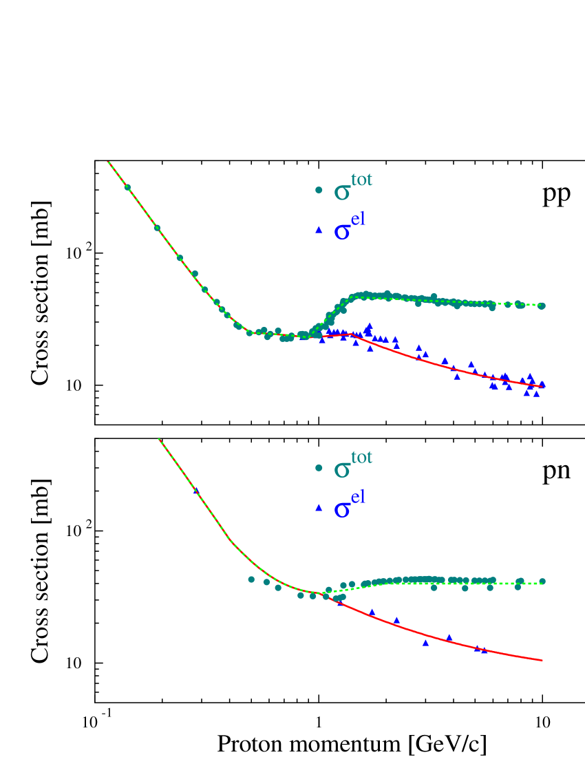
Figure 1: Total and elastic cross sections for proton-proton and proton-neutron scattering as a function of the proton lab momentum. The data are from Ref. [38]. The solid (dashed) curve displays our global fit to the elastic (total) cross section.

3.3 Relativized Glauber model for $A(e,e^{\prime}p)$

In the relativized Glauber multiple scattering framework, the antisymmetrized $A$-body wave function in the final state reads

$$\Psi^{\vec{k}_{p},m_{s}}_{A}\left(\vec{r},\vec{r}_{2},\vec{r}_{3},\ldots\vec{r}_{A}\right) \sim {\widehat{\mathcal{A}}}\Biggl{[}{\widehat{\mathcal{S}}\left(\vec{r},\vec{r}_{2},\vec{r}_{3},\ldots\vec{r}_{A}\right)}\left[\begin{array}[]{c}1\\ \frac{1}{E+M}\vec{\sigma}\cdot\vec{p}\end{array}\right]e^{i\vec{k}_{p}\cdot\vec{r}}\chi_{\frac{1}{2}m_{s}}$$ (43)

$$\times\Psi_{A-1}^{J_{R}\;M_{R}}\left(\vec{r}_{2},\vec{r}_{3},\ldots\vec{r}_{A}\right)\Biggr{]}\;,$$

where $\Psi_{A-1}^{J_{R}\;M_{R}}$ is the wave function characterizing the state in which the $A-1$ nucleus is created and ${\widehat{\mathcal{A}}}$ is the antisymmetrization operator. In the above expression, the subsequent elastic or “mildly inelastic” collisions of the struck proton with the “frozen” spectator nucleons, are implemented through the introduction of the following operator

$${\widehat{\mathcal{S}}\left(\vec{r},\vec{r}_{2},\vec{r}_{3},\ldots\vec{r}_{A}\right)}\equiv\prod_{j=2}^{A}\left[1-\Gamma\left(\vec{b}-\vec{b_{j}}\right)\theta\left(z_{j}-z\right)\right]\;,$$ (44)

where $\vec{r}\left(\vec{b},z\right)$ denotes the position of the struck particle and $\left(\vec{r}_{2},\vec{r}_{3},\ldots,\vec{r}_{A}\right)$ those of the (frozen) spectator protons and neutrons in the target. The step function $\theta\left(z_{j}-z\right)$ guarantees that the struck proton can only interact with the spectator protons and neutrons which it finds in its forward propagation path. Further, the profile function for $pN$ scattering is defined as

$$\Gamma(\vec{b})\equiv 1-e^{i\chi(\vec{b})}=\frac{{\sigma^{tot}_{pN}}(1-i{\epsilon_{pN}})}{4\pi\beta_{pN}^{2}}\>exp\left(-\frac{b^{2}}{2\beta_{pN}^{2}}\right)\;,$$

where the last equality can be derived from the expression (38). Two major assumptions underly the derivation of the operator of Eq. (44) : the eikonal approximation for the continuum wave function of the struck proton and the frozen approximation for the positions of the spectators. Indeed, one assumes that the ejectile passes through the nucleus in a very short time so that variations in the positions of the residual nucleons can be ignored. The operator of Eq. (44) represents the accumulated effect of the phase shifts contributed by each of the target scatterers as the ejectile progresses through the nucleus. The property of so-called phase-shift additivity is a direct consequence of the adopted one-dimensional nature of the relative motion, together with the neglect of three- and more-body forces, recoil effects and longitudinal momentum transfer.

The Dirac-Glauber $A(e,e^{\prime}p)$ transition amplitude can be written as

$$\left<J^{\mu}\right> = \int d\vec{r}\int d\vec{r}_{2}\ldots\int d\vec{r}_{A}$$ (45)

$$\times\left(\Psi^{\vec{k}_{p},m_{s}}_{A}\left(\vec{r},\vec{r}_{2},\vec{r}_{3},\ldots\vec{r}_{A}\right)\right)^{\dagger}\gamma^{0}J^{\mu}(r)e^{i\vec{q}\cdot\vec{r}}\Psi^{gs}_{A}\left(\vec{r},\vec{r}_{2},\vec{r}_{3},\ldots\vec{r}_{A}\right)\;,$$

where for convenience only the spatial coordinates are explicitly written. The difficulty of the evaluation of this matrix element stems from the fact that the multiple-scattering operator ${\widehat{\mathcal{S}}}$ is a genuine $A$-body operator. One popular approximation in Glauber inspired $A(e,e^{\prime}p)$ calculations, is expanding the A-body operator ${\widehat{\mathcal{S}}\left(\vec{r},\vec{r}_{2},\vec{r}_{3},\ldots\vec{r}_{A}\right)}$

$${\widehat{\mathcal{S}}\left(\vec{r},\vec{r}_{2},\vec{r}_{3},\ldots\vec{r}_{A}\right)}=1-\sum_{j=2}^{A}\theta(z_{j}-z)\Gamma(\vec{b}-\vec{b}_{j})$$ (46)

$$+ \sum_{j\neq k}^{A}\theta(z_{j}-z)\Gamma(\vec{b}-\vec{b}_{j})\theta(z_{k}-z)\Gamma(\vec{b}-\vec{b}_{k})$$

$$- \sum_{j\neq k\neq l=2}^{A}\theta(z_{j}-z)\Gamma(\vec{b}-\vec{b}_{j})\theta(z_{k}-z)\Gamma(\vec{b}-\vec{b}_{k})\theta(z_{l}-z)\Gamma(\vec{b}-\vec{b}_{l})$$

$$+ \ldots\;,$$

and truncating it at some order in $\Gamma$. Formally, this expansion bears a strong resemblance with the Mayer-Ursell expansion used in modeling the correlation effects in the theory of real gases and liquids. In the above expression, the unity operator (first term) reflects the situation whereby the ejectile is not subject to scatterings in its way out of the nucleus. The second term, which is linear in the profile function, accounts for processes whereby the struck nucleon scatters on one single spectator nucleon before turning asymptotically free (single-scattering process). Higher-order terms in the expansion refer to processes whereby the ejected proton subsequently scatters with two, three, $\ldots$, A-1 spectator nucleons. Evaluating the different terms in the above expansion allows one to estimate the effect of single-, double, triple-, $\ldots$ scatterings. For heavier nuclei, truncating the expansion at first order in $\Gamma$ appears as a rather questionable procedure. In Section 4 results obtained with the truncated (Eq. (46)) and complete (Eq. (44)) Dirac-Glauber multiple-scattering operator will be compared.

In evaluating the Dirac-Glauber transition amplitude of Eq. (45) we have introduced a minimal amount of approximations. In line with the assumptions underlying the RDWIA approaches we adopt a mean-field approximation for the nuclear wave functions. For the sake of brevity of the notations, in the forthcoming derivations we consider the case $A=3$. A generalization to arbitrary mass number $A$ is rather straightforward. Further, we will assume that the nuclear current $J^{\mu}$ is a one-body operator. As both the initial and final wave functions are fully antisymmetrized, one can choose the operator $J^{\mu}$ to act on one particular coordinate and write without any loss of generality $\left(\vec{r}\;^{\prime}\equiv(\vec{b}^{\prime}(x^{\prime},y^{\prime}),z^{\prime})\right)$

$$\left<J^{\mu}\right> = A\frac{1}{A!}\int d\vec{r}\;^{\prime}\int d\vec{r}_{2}\hskip 0.28453pt^{\prime}\int d\vec{r}_{3}\hskip 0.28453pt^{\prime}\sum_{k,l,m\in\left\{k_{p}m_{s},\alpha_{2},\alpha_{3}\right\}}\;\;\sum_{n,o,p\in\left\{\alpha_{1},\alpha_{2},\alpha_{3}\right\}}\epsilon_{klm}^{*}\epsilon_{nop}$$ (47)

$$\times\phi_{k}^{\dagger}\left(\vec{r}\;^{\prime}\right)\phi_{l}^{\dagger}\left(\vec{r}_{2}\hskip 0.28453pt^{\prime}\right)\phi_{m}^{\dagger}\left(\vec{r}_{3}\hskip 0.28453pt^{\prime}\right)e^{i\vec{q}\cdot\vec{r}\;^{\prime}}\gamma_{0}$$

$$\times J^{\mu}(\vec{r}\;^{\prime})\left[1-\theta\left(z^{\prime}_{2}-z^{\prime}\right)\Gamma\left(\vec{b}^{\prime}_{2}-\vec{b}^{\prime}\right)\right]^{\dagger}\left[1-\theta\left(z^{\prime}_{3}-z^{\prime}\right)\Gamma\left(\vec{b}^{\prime}_{3}-\vec{b}^{\prime}\right)\right]^{\dagger}$$

$$\times\phi_{n}\left(\vec{r}\;^{\prime}\right)\phi_{o}\left(\vec{r}_{2}\hskip 0.28453pt^{\prime}\right)\phi_{p}\left(\vec{r}_{3}\hskip 0.28453pt^{\prime}\right)\;,$$

with $\epsilon_{ijk}$ the Levi-Civita symbol, and where we have introduced a frame $(x^{\prime},y^{\prime},z^{\prime})$ defined by the following unit vectors

$$\hat{z}^{\prime}=\frac{\vec{k}_{p}}{\mid\vec{k}_{p}\mid}\;\;\;\;,\;\;\hat{y}^{\prime}=\frac{\vec{k}_{p}\times\vec{q}}{\mid\vec{k}_{p}\times\vec{q}\mid}\;\;\;\;,\;\;\hat{x}^{\prime}=\hat{z}^{\prime}\times\hat{y}^{\prime}\;.$$ (48)

The plane $(x^{\prime},z^{\prime})$ coincides with what is usually known as the hadron reaction plane in $A(e,e^{\prime}p)$ reactions.

Adopting a mean-field picture, the initial $A$-nucleon wave function is of the form

$$\Psi^{gs}_{A}\left(\vec{r}_{1},\vec{r}_{2},\vec{r}_{3}\right)=\frac{1}{\sqrt{A!}}\left|\begin{array}[]{ccc}\;\;\phi_{\alpha_{1}}\left(\vec{r}_{1}\right)&\;\;\phi_{\alpha_{2}}\left(\vec{r}_{1}\right)&\;\;\phi_{\alpha_{3}}\left(\vec{r}_{1}\right)\\ \;\;\phi_{\alpha_{1}}\left(\vec{r}_{2}\right)&\;\;\phi_{\alpha_{2}}\left(\vec{r}_{2}\right)&\;\;\phi_{\alpha_{3}}\left(\vec{r}_{2}\right)\\ \;\;\phi_{\alpha_{1}}\left(\vec{r}_{3}\right)&\;\;\phi_{\alpha_{2}}\left(\vec{r}_{3}\right)&\;\;\phi_{\alpha_{3}}\left(\vec{r}_{3}\right)\end{array}\right|\;.$$ (52)

For spherically symmetric potentials, the solutions $\phi_{\alpha}\left(\vec{r}\right)$ to a single-particle Dirac equation entering this Slater determinant have the form [39]

$$\phi_{\alpha}\left(\vec{r},\vec{\sigma}\right)\equiv\phi_{n\kappa m}(\vec{r},\vec{\sigma})=\left[\begin{array}[]{c}i\frac{G_{n\kappa}(r)}{r}\;{\mathcal{Y}}_{\kappa m}(\Omega,\vec{\sigma})\\ -\frac{F_{n\kappa}(r)}{r}\;{\mathcal{Y}}_{-\kappa m}(\Omega,\vec{\sigma})\end{array}\right]\;,$$ (53)

where $n$ denotes the principal, $\kappa$ and $m$ the generalized angular momentum quantum numbers. The ${\mathcal{Y}}_{\pm\kappa m}$ are the spin spherical harmonics and determine the angular and spin parts of the wave function,

$${\mathcal{Y}}_{\kappa m}(\Omega,\vec{\sigma})=\sum_{m_{l}m_{s}}\left<lm_{l}\frac{1}{2}m_{s}\mid jm\right>Y_{lm_{l}}(\Omega)\chi_{\frac{1}{2}m_{s}}(\vec{\sigma})\;,$$

$$j=|\kappa|-\frac{1}{2}\;,\hskip 22.76228ptl=\left\{\begin{array}[]{ll}\kappa,&\kappa>0\\ -(\kappa+1),&\kappa<0\;.\end{array}\right.$$ (56)

The final $A$-body wave function reads

$$\Psi^{\vec{k}_{p},m_{s}}_{A}\left(\vec{r}_{1},\vec{r}_{2},\vec{r}_{3}\right) = \frac{1}{\sqrt{A!}}\left|\begin{array}[]{ccc}\;\;{\widehat{\mathcal{S}}}\left(\vec{r}_{1},\vec{r}_{2},\vec{r}_{3}\right)\;\;\phi_{k_{p}m_{s}}\left(\vec{r}_{1}\right)&\;\;\phi_{\alpha_{2}}\left(\vec{r}_{1}\right)&\;\;\phi_{\alpha_{3}}\left(\vec{r}_{1}\right)\\ \;\;{\widehat{\mathcal{S}}}\left(\vec{r}_{2},\vec{r}_{1},\vec{r}_{3}\right)\;\;\phi_{k_{p}m_{s}}\left(\vec{r}_{2}\right)&\;\;\phi_{\alpha_{2}}\left(\vec{r}_{2}\right)&\;\;\phi_{\alpha_{3}}\left(\vec{r}_{2}\right)\\ \;\;{\widehat{\mathcal{S}}}\left(\vec{r}_{3},\vec{r}_{1},\vec{r}_{2}\right)\;\;\phi_{k_{p}m_{s}}\left(\vec{r}_{3}\right)&\;\;\phi_{\alpha_{2}}\left(\vec{r}_{3}\right)&\;\;\phi_{\alpha_{3}}\left(\vec{r}_{3}\right)\end{array}\right|\;.$$ (60)

Relative to the target nucleus ground state written in Eq. (52), the wave function of Eq. (LABEL:eq:finalstate) refers to the situation whereby the struck proton resides in a state “$\alpha_{1}$”, leaving the residual $A-1$ nucleus as a hole state in that particular single-particle level.

Assuming that the profile function $\Gamma$ does not contain spin-dependent terms, one can safely assume that for elastic and mildly inelastic scatterings

$$\int d\vec{r}_{1}\hskip 0.28453pt^{\prime}\int d\vec{r}_{2}\hskip 0.28453pt^{\prime}\phi_{k}^{\dagger}\left(\vec{r}_{1}\hskip 0.28453pt^{\prime}\right)\phi_{l}^{\dagger}\left(\vec{r}_{2}\hskip 0.28453pt^{\prime}\right)J^{\mu}(\vec{r}_{1}\hskip 0.28453pt^{\prime})$$ (62)

$$\times\left[1-\theta\left(z_{2}^{\prime}-z_{1}^{\prime}\right)\Gamma\left(\vec{b}_{2}^{\prime}-\vec{b}_{1}^{\prime}\right)\right]^{\dagger}\phi_{n}\left(\vec{r}_{1}\hskip 0.28453pt^{\prime}\right)\phi_{o}\left(\vec{r}_{2}\hskip 0.28453pt^{\prime}\right)$$

$$\approx\delta_{lo}\int d\vec{r}_{1}\hskip 0.28453pt^{\prime}\int d\vec{r}_{2}\hskip 0.28453pt^{\prime}\phi_{k}^{\dagger}\left(\vec{r}_{1}\hskip 0.28453pt^{\prime}\right)J^{\mu}(\vec{r}_{1}\hskip 0.28453pt^{\prime})$$

$$\times\left[1-\theta\left(z_{2}^{\prime}-z_{1}^{\prime}\right)\Gamma\left(\vec{b}_{2}^{\prime}-\vec{b}_{1}^{\prime}\right)\right]^{\dagger}\phi_{n}\left(\vec{r}_{1}\hskip 0.28453pt^{\prime}\right)\left|\phi_{o}\left(\vec{r}_{2}\hskip 0.28453pt^{\prime}\right)\right|^{2}\;.$$

Inserting this expression in Eq. (47) one obtains

$$\left<J^{\mu}\right> = A\frac{1}{A!}\int d\vec{r}\;^{\prime}\int d\vec{r}_{2}\hskip 0.28453pt^{\prime}\int d\vec{r}_{3}\hskip 0.28453pt^{\prime}\sum_{l,m\in\left\{\alpha_{2},\alpha_{3}\right\}}\epsilon_{(k_{p}m_{s})lm}^{*}\epsilon_{\alpha_{1}lm}$$ (63)

$$\times\phi_{k_{p}m_{s}}^{\dagger}\left(\vec{r}\;^{\prime}\right)\left|\phi_{l}\left(\vec{r}_{2}\hskip 0.28453pt^{\prime}\right)\right|^{2}\left|\phi_{m}\left(\vec{r}_{3}\hskip 0.28453pt^{\prime}\right)\right|^{2}e^{i\vec{q}\cdot\vec{r}\;^{\prime}}\gamma_{0}J^{\mu}(\vec{r}\;^{\prime})\phi_{\alpha_{1}}\left(\vec{r}\;^{\prime}\right)$$

$$\times\left[1-\theta\left(z_{2}^{\prime}-z^{\prime}\right)\Gamma\left(\vec{b}_{2}^{\prime}-\vec{b}^{\prime}\right)\right]^{\dagger}\left[1-\theta\left(z_{3}^{\prime}-z^{\prime}\right)\Gamma\left(\vec{b}_{3}^{\prime}-\vec{b}^{\prime}\right)\right]^{\dagger}\;.$$

This leads to our final result for the Dirac-Glauber $A(e,e^{\prime}p)$ transition amplitude

$$\left<J^{\mu}\right>=\int d\vec{r}\phi_{k_{p}m_{s}}^{\dagger}\left(\vec{r}\right)\mathcal{G}^{\dagger}(\vec{b},z)\gamma^{0}J^{\mu}(\vec{r})e^{i\vec{q}\cdot\vec{r}}\phi_{\alpha_{1}}\left(\vec{r}\right)\;,$$ (64)

where the Dirac-Glauber phase $\mathcal{G}(\vec{b},z)$ is defined in the following fashion

$$\mathcal{G}(\vec{b},z)=\prod_{\alpha_{occ}\neq\alpha}\left[1-\int d\vec{r}\hskip 0.28453pt^{\prime}\left|\phi_{\alpha_{occ}}\left(\vec{r}\hskip 0.28453pt^{\prime}\right)\right|^{2}\theta\left(z^{\prime}-z\right)\Gamma\left(\vec{b}^{\prime}-\vec{b}\right)\right]\;.$$ (65)

In this expression, the product extends over all occupied single-particle states, except for the one from which the nucleon is ejected. The RPWIA approximation would correspond with putting $\mathcal{G}=1$ in the expression for the matrix element of Eq. (64).

The numerical evaluation of the Glauber phase $\mathcal{G}(\vec{b},z)$ is rather challenging if no additional approximations are introduced. A Monte Carlo integration method was suggested in Ref [40]. In our numerical calculations we did not introduce any further approximations and found it most appropriate to evaluate the scattering amplitudes and Glauber phases in the frame defined by the unit vectors of Eq. (48). Inserting the expression for the Dirac single-particle wave functions $\phi_{\alpha}$ of Eq. (53) in the Eq. (65) for the Glauber phase, one gets ($d\vec{r}\hskip 0.85358pt^{\prime}\equiv dz^{\prime}b^{\prime}db^{\prime}d\phi_{b^{\prime}}$)

$$\mathcal{G} (\vec{b},z)=\prod_{\alpha_{occ}\neq\alpha}\Biggl{\{}1-\frac{\sigma^{tot}_{pN}(1-i\epsilon_{pN})}{4\pi\beta_{pN}^{2}}\int_{0}^{\infty}b^{\prime}db^{\prime}\int_{0}^{\infty}dz^{\prime}\theta(z^{\prime}-z)$$ (66)

$$\times\Biggl{(}\biggl{[}\frac{G_{n\kappa}\left(r^{\prime}(b^{\prime},z^{\prime})\right)}{r^{\prime}(b^{\prime},z^{\prime})}\mathcal{Y}_{\kappa m}(\Omega(b^{\prime},z^{\prime}),\vec{\sigma})\biggr{]}^{2}$$

$$+\biggl{[}\frac{F_{n\kappa}\left(r^{\prime}(b^{\prime},z^{\prime})\right)}{r^{\prime}(b^{\prime},z^{\prime})}\mathcal{Y}_{\kappa m}(\Omega(b^{\prime},z^{\prime}),\vec{\sigma})\biggr{]}^{2}\Biggr{)}$$

$$\times\exp\left[-\frac{(b-b^{\prime})^{2}}{2\beta_{pN}^{2}}\right]\int_{0}^{2\pi}d\phi_{b^{\prime}}\exp\biggl{[}\frac{-bb^{\prime}}{\beta_{pN}^{2}}2{\sin}^{2}\left(\frac{\phi_{b}-\phi_{b^{\prime}}}{2}\right)\biggr{]}\Biggr{\}}\;.$$

Standard numerical integration techniques were adopted to evaluate the integrals occurring in this equation. It is important to remark that cylindrical symmetry about the $z^{\prime}$ axis makes the above expression to be independent of $\phi_{b}$. As a result the relativistic Glauber depends on only two independent variables $(b,z)$. In the above expression (66) each of the frozen spectator nucleons is identified by its quantum numbers $(n,\kappa,m)$ and its corresponding Dirac wave function $\phi_{n\kappa m}(\vec{r},\vec{\sigma})$. In most Glauber-based calculations, an additional averaging over the positions of the spectator nucleons is introduced. This procedure amounts to replacing in Eq. (66) the characteristic spatial distributions of each of the spectator nucleons described by the functions $F_{n\kappa}(r)$ and $G_{n\kappa}(r)$ by an average density distribution for the target nucleus

$$\mathcal{G}(b,z) = \Biggl{\{}1-\frac{\sigma^{tot}_{pN}(1-i\epsilon_{pN})}{4\pi\beta_{pN}^{2}}\int_{0}^{\infty}b^{\prime}db^{\prime}T_{B}(b^{\prime},z)\exp\left[-\frac{(b-b^{\prime})^{2}}{2\beta_{pN}^{2}}\right]$$ (67)

$$\times\int_{0}^{2\pi}d\phi_{b^{\prime}}\exp\biggl{[}\frac{-bb^{\prime}}{\beta_{pN}^{2}}2{\sin}^{2}\left(\frac{\phi_{b}-\phi_{b^{\prime}}}{2}\right)\biggr{]}\Biggr{\}}^{A-1}\;.$$

The function $T_{B}(b^{\prime},z)$ which was introduced in the above expressions is known as the “thickness function” and reads

$$T_{B}(b^{\prime},z)=\frac{1}{A}\int_{0}^{+\infty}dz^{\prime}\theta\left(z^{\prime}-z\right)\rho_{B}(r^{\prime}(b^{\prime},z^{\prime}))\;,$$ (68)

where the relativistic radial baryon density $\rho_{B}(r)$ is defined in the standard fashion

$$\rho_{B}(r)\equiv\left<\overline{\Psi_{A}^{gs}}\gamma_{0}\Psi_{A}^{gs}\right> = \sum_{\alpha_{occ}}\int d\vec{\sigma}d\Omega\left(\phi_{\alpha_{occ}}(\vec{r},\vec{\sigma})\right)^{\dagger}\left(\phi_{\alpha_{occ}}(\vec{r},\vec{\sigma})\right)\;$$ (69)

$$= \sum_{n\kappa}\frac{(2j+1)}{4\pi r^{2}}\biggl{[}\left|G_{n\kappa}(r)\right|^{2}+\left|F_{n\kappa}(r)\right|^{2}\biggr{]}\;,$$

and the sum over $n\kappa$ extends over all occupied states.

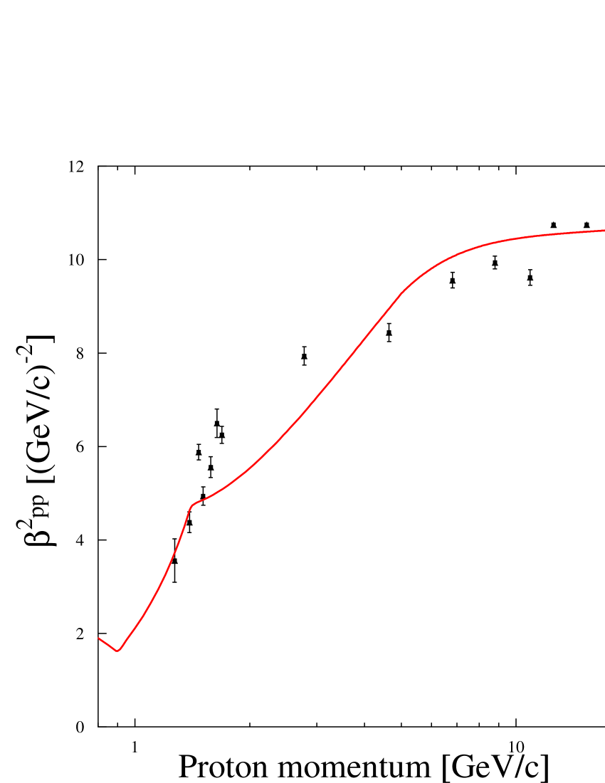
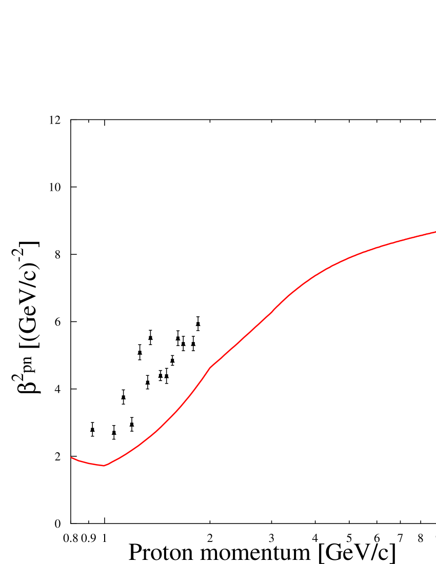
Figure 2: The Glauber slope parameters $\beta_{pp}^{2}$ and $\beta_{pn}^{2}$ as obtained from Eq. (70) with the global fits contained in Fig. 1. The data are from Refs. [41] (proton-neutron) and [42] (proton-proton) and are determined from the small-angle $t$ dependence of the measured differential cross sections.

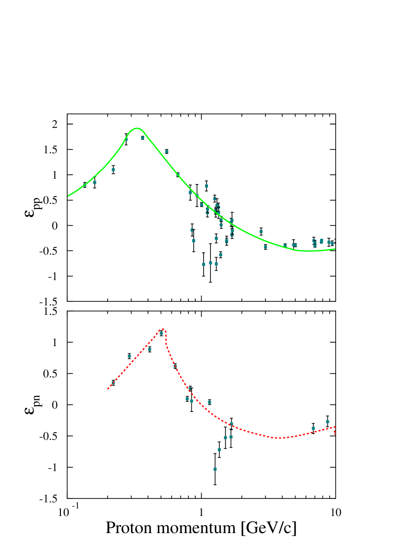
Figure 3: The ratios of the real to imaginary parts of the central amplitude $f_{pN}^{c}$ for proton-proton and proton-neutron scattering as a function of the proton lab momentum. The curves are our global fits to the data points. The data are from the review paper of Ref. [37].

3.4 Glauber parameters

We refer to $A(e,e^{\prime}p)$ results obtained with a scattering state of the form of Eq. (43) as a relativistic multiple-scattering Glauber approximation (RMSGA) calculation. It is worth stressing that in contrast to the RDWIA models, all parameters entering the calculation of the scattering states in the RMSGA $A(e,e^{\prime}p)$ model can be directly determined from the elementary proton-proton and proton-neutron scattering data. In practice, for a given ejectile’s lab momentum $\mid\vec{k}_{p}\mid$ the following input is required : the total proton-proton ${\sigma^{tot}_{pp}}$ and proton-neutron ${\sigma^{tot}_{pn}}$ cross sections, the corresponding slope parameters (${\beta_{pp}^{2}}$ and ${\beta_{pn}^{2}}$) and the ratios of the real to imaginary part of the scattering amplitude (${\epsilon_{pp}}$ and ${\epsilon_{pn}}$). We obtain the numbers ${\sigma^{tot}_{pN}}$, ${\beta_{pN}^{2}}$ and ${\epsilon_{pN}}$ through interpolation of the data base available from the Particle Data Group [38]. The slope parameters $\beta_{pp}^{2}$ and $\beta_{pn}^{2}$ may be found by analyzing the shape of the differential cross sections assuming that the contribution from the spin-dependent terms is negligible. At proton momenta $p_{p}\leq$ 1 GeV the slope parameters found directly from experiment and phase-shift analysis differ significantly due to a large contribution from the spin-dependent scattering amplitude [37]. At higher energies this difference drops quickly indicating that spin effects are small in that region. In our calculations, the slope parameters are obtained from the ratio of the elastic $\sigma_{pN}^{el}$ to the total $\sigma_{pN}^{tot}$ cross section through the following relation

$$\beta_{pN}^{2}\approx\frac{\left(\sigma^{tot}_{pN}\right)^{2}\left(\epsilon_{pN}^{2}+1\right)}{16\pi\sigma^{el}_{pN}}\;.$$ (70)

In Fig. 2 we compare the slope parameters obtained through this formulae with those extracted directly from the $t$ dependence of the differential $pN$ cross sections. The curves in Fig. 2 use the above formulae (70) and our global fits to $\sigma^{tot}_{pN}$, $\sigma^{el}_{pN}$ and $\epsilon_{pN}$ shown in Figs. 1 and 3. For proton-proton scattering the situation emerges to be very satisfactory.

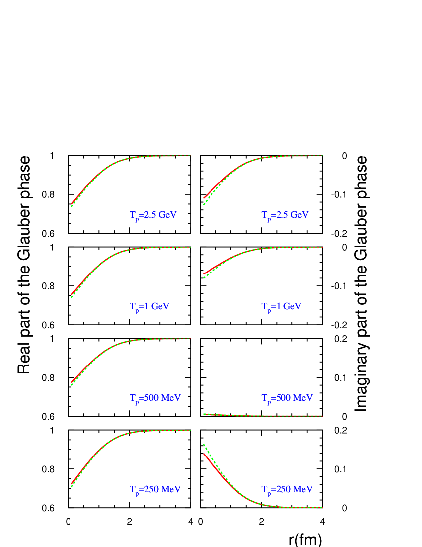
Figure 4: The radial dependence of the real and imaginary part of the computed Glauber phase $\mathcal{G}$ along the direction of the ejected particle ( $\theta=0^{\circ}$) for proton emission from ⁴He at various proton kinetic energies $T_{p}$. Results with the expression of Eq. (46) truncated to the first order in $\Gamma$ (dashed line) are compared to the full result (solid line).

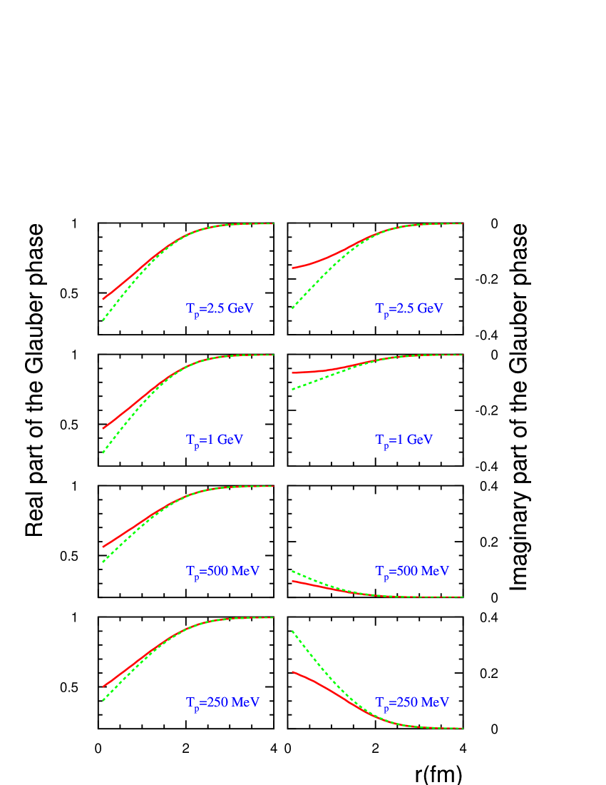
Figure 5: As in Figure 4 but now for ¹²C.

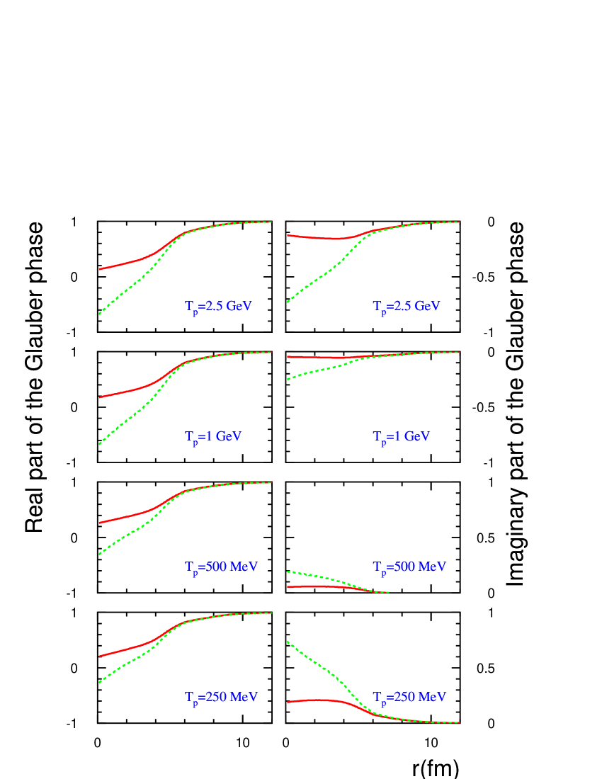
Figure 6: As in Figure 4 but now for ²⁰⁸Pb.

4 Numerical results for relativistic Glauber phases

4.1 Single- and multiple-scattering effects

In many works, in the calculation of the Glauber phases only a limited amount of terms in the expansion of Eq. (46) is retained. In some cases, the operator $\mathcal{S}$ is replaced by the term which is first order in $\Gamma$. This reduces the treatment of the FSI effects to one-body operators and corresponds with retaining the cumulative effect of free passage through the target in addition to single scatterings. We wish to compare Glauber phases obtained with the exact operator with those that are produced when allowing only single scatterings. The Glauber phase, as it was defined in Eq. (65) depends on the two variables $(b,z)$ and is independent of $\phi_{b}$. We wish to remind the reader that for convenience of the numerical integrations the $z^{\prime}$-axis is chosen to point along the asymptotic direction $\vec{k}_{p}$ of the ejectile.

In Figs. 4,  5, 6 results are displayed for the computed real and imaginary part of

$$\mathcal{G}(r,\theta)=\mathcal{G}\left(b=\sqrt{r^{2}-r^{2}\cos^{2}\theta}\;,z=r\cos\theta)\right)\;,$$ (71)

for the target nuclei ⁴He, ¹²C and ²⁰⁸Pb and $\theta=0^{o}$. Here, $\theta$ denotes the polar angle with respect to the axis defined by the asymptotic momentum of the ejected particle. We remind that in the absence of final-state interactions the real part of the Glauber phase equals one, whereas the imaginary part vanishes identically. As becomes clear from Fig. 4, the approximation of retaining only single-rescattering terms, emerges to be a reasonable approximation for the ⁴He target nucleus. As a consequence, for ⁴He the average number of rescatterings can be inferred not to be larger than one. For a given ejectile’s momentum, the average number of scatterers which it encounters in its way out of the nucleus is expected to grow like $A^{1/3}$. Given that for $A=4$ the average number of rescatterings is not larger than 1, one can infer that for a heavy nucleus like ²⁰⁸Pb the scattering series of Eq. (46) will receive sizeable contributions up to the fourth order in $\Gamma$. This complies with the numbers quoted in Table 1 of Ref. [25]. As can be inferred from Figs. 4, 5, 6, single rescatterings dominate the real and imaginary part of the Glauber phase at the nuclear surface. In the interior of the nucleus, single- and the summed higher-order scattering terms come with an opposite sign for all target nuclei studied. As a matter of fact, even for a nucleus like ¹²C, the truncation to single scatterings results in a sizeable overestimation of the FSI effects. The real part of the Glauber phase exhibits relatively little $T_{p}$ dependence over the range 0.25 - 2.00 GeV covered in the figures. The imaginary part, on the other hand, changes sign as one exceeds $T_{p}=0.5$ GeV and enters a highly inelastic regime. This observed change in the relative sign between the real and imaginary parts of the Glauber phase is governed by the $T_{p}$ dependence of the parameters $\epsilon_{pp}$ and $\epsilon_{pn}$ as is shown in Fig. 3.

When evaluating the $(e,e^{\prime}p)$ matrix elements and performing the integrations over $r$ and $\theta$, the functions displayed in Figs. 4 - 6 quantify the effects stemming from the FSI along the direction defined by the asymptotic momentum of the ejectile. For the Glauber phases, the radial coordinate “$r$” can be interpreted as the distance relative to the center of the target nucleus where the photon hits the target nucleus. For a given $r$, an additional non-trivial integration over the polar angles $\theta$ has to be performed. Here, $0^{o}\leq\theta\leq 90^{o}$ ($90^{o}\leq\theta\leq 180^{o}$) refers to a situation where the photon hits the nucleon in the forward (backward) hemisphere with respect to the direction defined by $\vec{k}_{p}$. The dependence of the real and imaginary part of the Dirac Glauber phase on the polar angle $\theta$ is illustrated in Fig. 7 for emission of 1 GeV protons from ⁴He. The $\theta=180^{o}$ case corresponds with a peculiar event whereby the photon couples to the proton along the direction defined by $-\vec{k}_{p}$. For $\theta=180^{o}$ and increasing $r$, the photon initially hits the proton at the outskirts of the nucleus and the proton has to travel through the whole nucleus before it becomes asymptotically free at the opposite side. It speaks for itself that these kinematical situations induce the largest FSI effects but cannot be expected to provide large contributions to the integrated matrix elements.

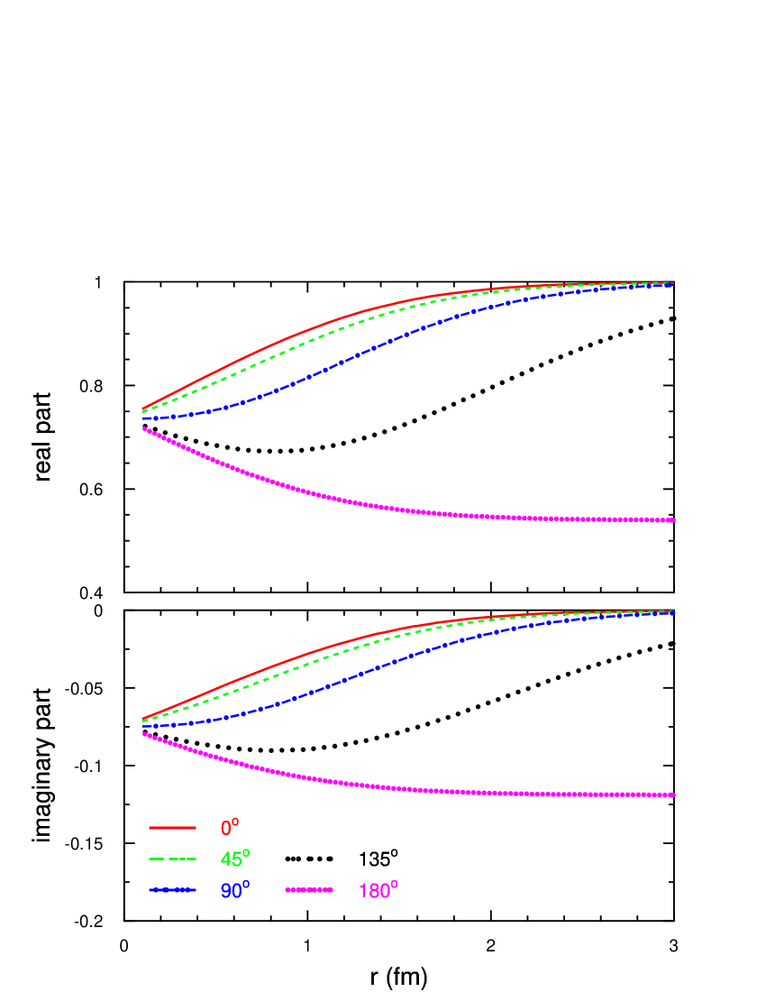
Figure 7: The radial dependence of the real and imaginary part of the computed Glauber phase $\mathcal{G}$ at various values of $\theta$ and $T_{p}$=1 GeV for proton emission out of ⁴He.

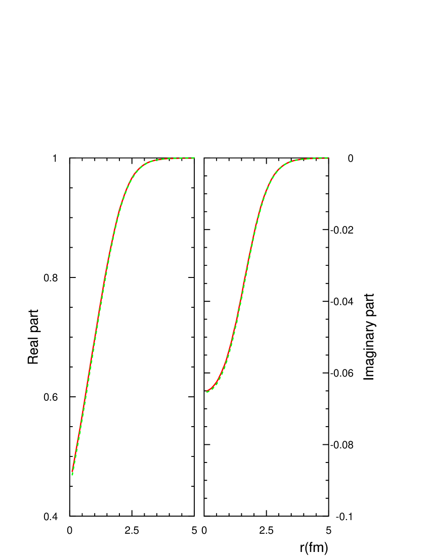
Figure 8: The effect of the lower components in the wave functions for the scattering centers on the computed Glauber phase $\mathcal{G}$ at $\theta=0^{o}$ and $T_{p}=1$ GeV for proton emission out of ¹²C. Results with ignoring the lower components (dashed line) are compared to the full result (solid line).

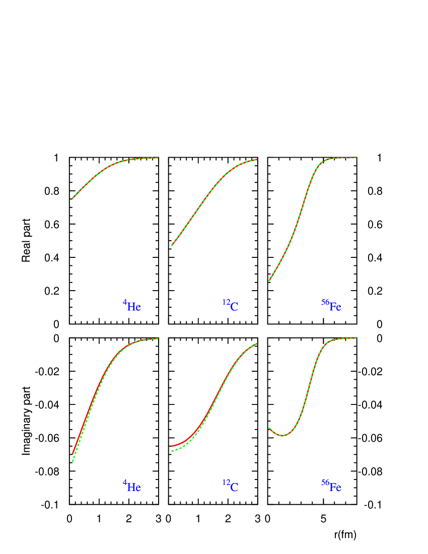
Figure 9: Effect of replacing the wave functions for the individual scattering centers by an average density on the computed Glauber phase $\mathcal{G}$. The results are obtained for $\theta=0^{o}$ and $T_{p}=1$ GeV for proton emission out of ⁴He, ¹²C and ⁵⁶Fe. Results with the approximated expression from Eq. (66) (dashed line) are compared to the exact result from Eq. (65) (solid line).

4.2 Relativistic and density effects

The role of relativity in the description of the FSI can be estimated by neglecting the small components $F_{n\kappa}(r)$ in the relativistic wave functions for the individual scattering nucleons in Eq. (65) and comparing it to the exact result. We have performed several of these calculations for a variety of target nuclei. One representative result is displayed in Fig. 8. In general, the relativistic lower wave function components for the scattering centers (i.e. the nucleons residing in the daughter nucleus) are observed to have a minor impact on the predictions for both the real and imaginary part of the Glauber phase. In the next section, however, it will be shown that inclusion of the lower relativistic components is essential for some $A(e,e^{\prime}p)$ observables. From the results presented here, it can be excluded that this could be attributed to a relativistic effect in the description of the final-state interactions.

Besides the neglect of relativistic effects, most Glauber calculations use an average nuclear density to describe the spatial distribution for each of the frozen nucleons from which the ejectile can scatter. This approximation was outlined at the end of Sect.  3.3. One may naively expect that this “averaging” at the wave-function level becomes increasingly accurate as the target mass number $A$ increases. As a matter of fact, the results displayed in Fig. 9 illustrate that the quoted approximation is a valid one even for a light nucleus like ⁴He. Inspecting Fig. 9, only in the absorptive part for ⁴He and ¹²C a minor overestimation gets introduced through the averaging procedure.

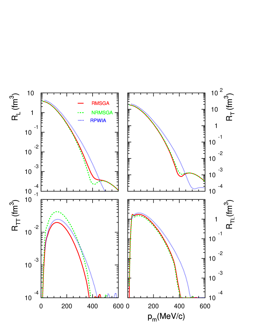
Figure 10: Separated ⁴He$(e,e^{\prime}p)^{3}$H response functions versus missing momentum in constant $(q,\omega)$-kinematics under quasi-elastic conditions. The electron kinematics was $\epsilon$=4.80 GeV, $q$=1.50 GeV and $\omega$=0.84 GeV (i.e., $Q^{2}$=1.54 (GeV)²).

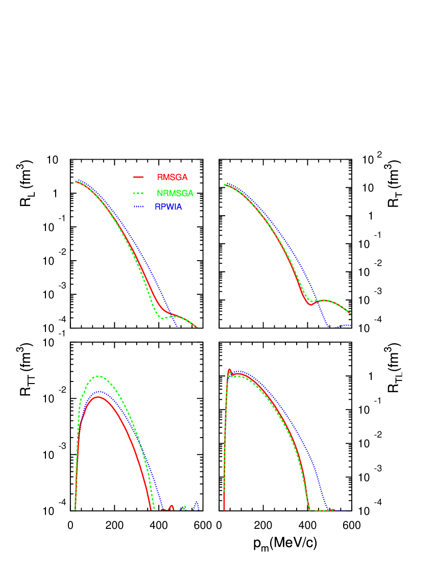
Figure 11: Separated ⁴He$(e,e^{\prime}p)^{3}$H structure functions versus missing momentum in constant $(q,\omega)$-kinematics under quasi-elastic conditions. The electron kinematics was $\epsilon$=2.442 GeV, $q$=1.696 GeV and $\omega$=1 GeV (i.e., $Q^{2}$=1.88 (GeV)²).

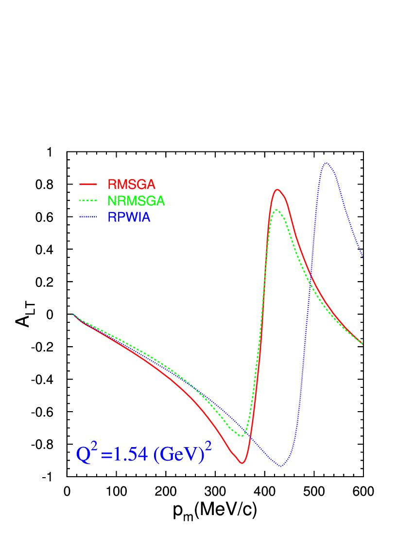
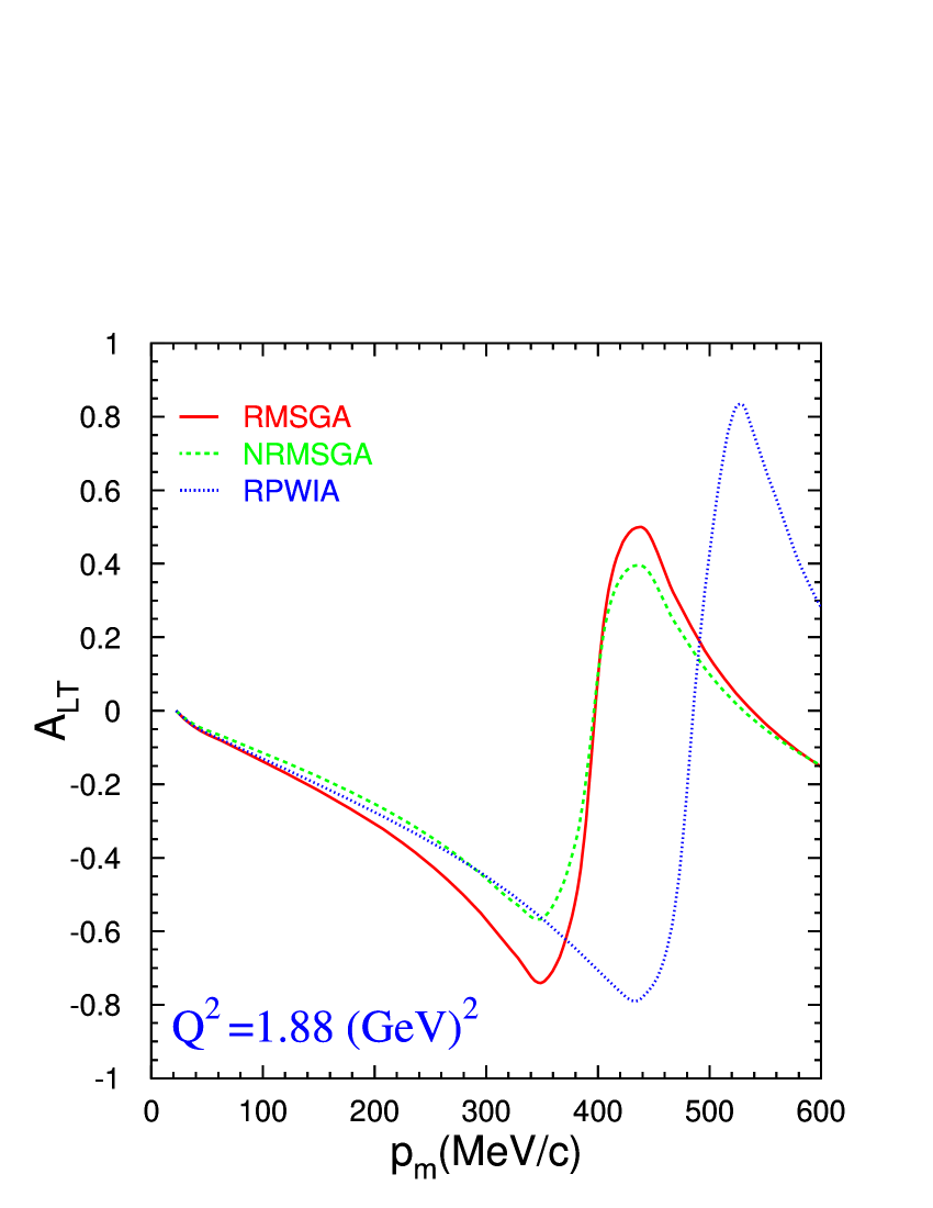
Figure 12: The $A_{TL}$ left-right asymmetries as a function of the missing momentum corresponding with the kinematics of Figs. 10 and 11.

5 Numerical results for ⁴He$(e,e^{\prime}p)$ structure functions

In conventional nuclear-physics models, by which we understand models which are based on hadronic degrees-of-freedom, the ⁴He nucleus plays a key role. Indeed, it is the simplest nuclear system in which all basic characteristics of “complex” nuclei exist. Accordingly, it comes at no surprise that the ⁴He$(e,e^{\prime}p)^{3}$H reaction plays a pivotal role in investigations into the short-range structure of nuclei [43] and medium-modification effects [5]. In Figs. 10 and 11 we display some predictions for the separated ⁴He$(e,e^{\prime}p)^{3}$H response functions in kinematics presently accessible at the Thomas Jefferson National Accelerator Facility. As a matter of fact, the kinematics corresponding with Fig. 10 coincides with a scheduled experiment at this facility [43].

Non-relativistic $A(e,e^{\prime}p)$ calculations typically miss, amongst other things, the effect from the coupling between the lower components in the bound and scattering states. As a matter of fact, we interpret the contribution from the coupling between the lower component in the bound ($\phi_{\alpha_{1}}$) and scattering state ($\phi_{k_{p}m_{s}}$) to the matrix element of Eq. (64) as a measure for the impact of relativistic effects. We denote $A(e,e^{\prime}p)$ results that are obtained after omitting this specific part as “NRMSGA”. We wish to stress that these “NRMSGA” calculations still use relativistic kinematics and bound and scattering states obtained by solving a Dirac equation. As can be appreciated from Figs. 10 and 11, the effect of the coupling between the lower components is marginal for the structure functions $\mathcal{R}_{L}$ and $\mathcal{R}_{T}$, but substantial for the two interference functions $\mathcal{R}_{TT}$ and $\mathcal{R}_{TL}$. These conclusions regarding the role of relativistic effects at low missing momenta confirms the major findings of numerous other investigations [15, 16]. Note that the genuine relativistic effect stemming from the coupling between the lower components is very prominent in the (non)-filling of the predicted dip in the cross section for $p_{m}\approx 410$  MeV. In order to illustrate the substantial impact of relativistic effects on some observables, Fig. 12 presents the so-called left-right asymmetry

$$A_{LT}=\frac{\sigma(\phi=0^{o})-\sigma(\phi=180^{o})}{\sigma(\phi=0^{o})+\sigma(\phi=180^{o})}=\frac{v_{TL}{\mathcal{R}}_{TL}}{\biggl{[}v_{L}{\mathcal{R}}_{L}+v_{T}{\mathcal{R}}_{T}+v_{TT}{\mathcal{R}}_{TT}\biggr{]}}\;,$$ (72)

corresponding with the kinematics of Figs. 10 and 11. As can be seen the genuine relativistic effect due to contribution from the the lower components in the bound and scattering state bring about a substantial increase in $A_{LT}$. As a matter of fact, the RMSGA $A_{LT}$ predictions of Fig. 12 are completely in line with the optical-potential RDWIA predictions by J. Udias contained in Ref. [43].

The relativistic plane wave impulse approximation (RPWIA) results of Figs. 10 - 12 are obtained after setting the Glauber phase $\mathcal{G}(b,z)$ equal to one in the matrix elements of Eq. (64). This corresponds with a calculation which ignores all FSI mechanisms but adopts relativistic kinematics, Dirac bound states, a relativistic plane wave for the ejectile and a relativistic current operator. At low missing momentum the FSI quenches the cross sections by 20 %, confirming the result of the non-relativistic Glauber calculations of Refs. [20], [44] and the calculations of Laget reported in Ref. [45]. Not surprisingly, with growing missing momentum the FSI effects become increasingly important. For example the dip in the RPWIA response functions at $p_{m}\approx 0.5$ GeV is shifted downwards by about 100 MeV and partially washed out.

6 Summary and conclusions

A fully unfactorized relativistic formulation of Glauber multiple-scattering theory for modeling exclusive $A(e,e^{\prime}p)$ processes has been presented. Formally, the model bears a strong resemblance with the RDWIA approaches which have been developed over the last number of decades. In contrast to the RDWIA models, the relativistic Glauber approximation for dealing with FSI mechanisms holds stronger links with the elementary proton-proton and proton-neutron processes and does not require the (phenomenological) input of optical potentials. Our fully unfactorized framework can accommodate all relativistic effects which are usually implemented in the RDWIA approaches. Like in the RDWIA models, the bound-state wave functions are solutions to a Dirac equation with scalar and vector potentials fitted to the ground-state nuclear properties, i.e. an approach commonly known as the $\sigma-\omega$ model.

The relative contribution from single- and multiple-scatterings to the integrated FSI mechanisms, has been investigated. For the target nucleus ⁴He, it turned out that single-scatterings give already a fair account of the complete scattering processes, and that double- and triple-scatterings are rare. For target nuclei heavier than ⁴He, the net effect of double-, triple- and quadruple-scatterings is found to affect the real and imaginary parts of the FSI induced phase with an opposite sign as compared to the single-scattering term. For ¹²C and heavier target nuclei, Glauber calculations restricted to single-scatterings substantially overestimate the FSI mechanisms. The lower components in the relativistic single-particle wave functions, on the other hand, are observed to have a negligible impact on the predictions for the distorting and absorptive effect of single- and multiple-scattering events which the ejected proton undergoes. This observation provides support for the non-relativistic Glauber approaches which have been widely adopted in nuclear transparency calculations for example. Also the frequently adopted simplification of replacing the squared nucleon wave functions for the individual scatterering centers in the target nucleus by some averaged nuclear density, was found to lead to results which approximate nicely the exact ones.

The developed RMSGA model has been applied to the exclusive ⁴He $+e\longrightarrow e^{\prime}+p+t$ process. The predicted RMSGA structure functions are found to follow similar trends in comparison to predictions from non-relativistic Glauber and relativistic optical-potential calculations. Extensions of the presented model include the implementation of short-range nucleon-nucleon correlations and color transparency effects. Work in this direction is in progress.

References

- [1] V. Pandharipande, I. Sick, P. deWitt Huberts, Rev. Mod. Phys. 69 (1997) 981.
- [2] H. Müther, A. Polls, Prog. Part. Nucl. Phys. 45 (2000) 243.
- [3] J. Gao et al., Phys. Rev. Lett. 84 (2000) 3265.
- [4] S. Malov et al., Phys. Rev. C 62 (2000) 057302.
- [5] S. Dieterich et al., Phys. Lett. B 500 (2001) 47.
- [6] K. Garrow et al., Phys. Rev. C 66 (2002) 044613.
- [7] S. Boffi, C. Giusti, F. Pacati, Phys. Rep. 226 (1993) 1.
- [8] J. Kelly, Adv. Nucl. Phys 23 (1996) 75.
- [9] A. Picklesimer, J. Van Orden, S. Wallace, Phys. Rev. C 32 (1985) 1312.
- [10] J. Johansson, H. Sherif, G. Lotz, Nucl. Phys. A 605 (1996) 517.
- [11] Y. Yin, D. Onley, L. Wright, Phys. Rev. C 45 (1992) 1311.
- [12] J. Udias, P. Sarriguren, E. Moya de Guerra, E. Garrido, J. Caballero, Phys. Rev. C 48 (1993) 2731.
- [13] A. Meucci, C. Giusti, F. Pacati, Phys. Rev. C 64 (2000) 64014605.
- [14] B. Serot, J. Walecka, Adv. Nucl. Phys. 16 (1986) 1.
- [15] J. Udias, J. Vignote, Phys. Rev. C 62 (2000) 034302.
- [16] M. Martínez, J. Caballero, T. Donnelly, Nucl. Phys. A 707 (2002) 83.
- [17] R. Glauber, G. Matthiae, Nucl. Phys. B 21 (1970) 135.
- [18] S. J. Wallace, Phys. Rev. C 12 (1975) 179.
- [19] D. Yennie, Interaction of high-energy photons with nuclei as a test of vector-meson-dominance, in: J. Cummings, D. Osborn (Eds.), Hadronic Interactions of Electrons and Photons, Academic, New York, 1971, p. 321.
- [20] O. Benhar, N. Nikolaev, J. Speth, A. Usmani, B. Zakharov, Nucl. Phys. A 673 (2000) 241.
- [21] C. Ciofi degli Atti, L. Kaptari, D. Treleani, Phys. Rev. C 63 (2001) 044601.
- [22] S. Jeschonnek, T. Donnelly, Phys. Rev. C 59 (1999) 2676.
- [23] A. Kohama, K. Yazaki, R. Seki, Nucl. Phys. A 662 (2000) 175.
- [24] L. Frankfurt, E. Moniz, M. Sargsyan, M. Strikman, Phys. Rev. C 51 (1995) 3435.
- [25] N. Nikolaev, A. Szcurek, J. Speth, J. Wambach, B. Zakharov, V. Zoller, Nucl. Phys. A 582 (1995) 665.
- [26] M. Petraki, E. Mavrommatis, O. Benhar, J. Clark, A. Fabrocini, S. Fantoni, Phys. Rev. C 67 (2003) 014605.
- [27] R. Amado, J. Piekarewicz, D. Sparrow, J. McNeil, Phys. Rev. C 28 (1983) 1663.
- [28] W. Greenberg, G. Miller, Phys. Rev. C 49 (1994) 2747.
- [29] D. Debruyne, J. Ryckebusch, W. Van Nespen, S. Janssen, Phys. Rev. C 62 (2000) 024611.
- [30] T. Donnelly, A. Raskin, Ann. Phys. 169 (1986) 247.
- [31] A. Raskin, T. Donnelly, Ann. Phys. 191 (1989) 78.
- [32] J. Bjorken, S. Drell, Relativistic Quantum Mechanics, Mc-Graw-Hill, New York, 1964.
- [33] E. Cooper, S. Hama, B. Clarck, R. Mercer, Phys. Rev. C 47 (1993) 297.
- [34] H. Ito, S. Koonin, R. Seki, Phys. Rev. C 56 (1997) 3231.
- [35] A. Bianconi, M. Radici, Phys. Lett. B 363 (1995) 24.
- [36] A. Bianconi, M. Radici, Phys. Rev. C 54 (1996) 3117.
- [37] G. Alkhazov, S. Belostotsky, A. Voroboyov, Phys. Rep. 42 (1978) 89.
-
[38]
K. Hagiwara, K. Hikasa, K. Nakamura, M. Tanabashi,
M. Aguilar-Benitez, C. Amsler, R. Barnett, P. Burchat, C. Carone,
C. Caso, G. Conforto, O. Dahl, M. Doser, S. Eidelman, J. Feng,
L. Gibbons, M. Goodman, C. Grab, D. Groom, A. Gurtu, K. Hayes,
J. Hernández-Rey, K. Honscheid, C. Kolda, M. Mangano, D. Manley,
A. Manohar, J. March-Russell, A. Masoni, R. Miquel, K. Mönig,
H. Murayama, S. Navas, K. Olive, L. Pape, C. Patrignani,
A. Piepke, M. Roos, J. Terning, N. Törnqvist, T. Trippe,
P. Vogel, C. Wohl, R. Workman, W.-M. Yao, B. Armstrong, P. Gee,
K. Lugovsky, S. Lugovsky, V. Lugovsky, M. Artuso, D. Asner,
K. Babu, E. Barberio, M. Battaglia, H. Bichsel, O. Biebel,
P. Bloch, R. Cahn, A. Cattai, R. Chivukula, R. Cousins, G. Cowan,
T. Damour, K. Desler, R. Donahue, D. Edwards, V. Elvira,
J. Erler, V. Ezhela, A. Fassò, W. Fetscher, B. Fields,
B. Foster, D. Froidevaux, M. Fukugita, T. Gaisser, L. Garren, H.-J.
Gerber, F. Gilman, H. Haber, C. Hagmann, J. Hewett,
I. Hinchliffe, C. Hogan, G. Höhler, P. Igo-Kemenes, J. Jackson,
K. Johnson, D. Karlen, B. Kayser, S. Klein, K. Kleinknecht,
I. Knowles, P. Kreitz, Y. Kuyanov, R. Landua, P. Langacker,
L. Littenberg, A. Martin, T. Nakada, M. Narain, P. Nason,
J. Peacock, H. Quinn, S. Raby, G. Raffelt, E. Razuvaev, B. Renk,
L. Rolandi, M. Ronan, L. Rosenberg, C. Sachrajda, A. Sanda,
S. Sarkar, M. Schmitt, O. Schneider, D. Scott, W. Seligman,
M. Shaevitz, T. Sjöstrand, G. Smoot, S. Spanier, H. Spieler,
N. Spooner, M. Srednicki, A. Stahl, T. Stanev, M. Suzuki,
N. Tkachenko, G. Valencia, K. van Bibber, M. Vincter, D. Ward,
B. Webber, M. Whalley, L. Wolfenstein, J. Womersley, C. Woody,
O. Zenin, Review of particle physics, Physical Review D 66 (2002) 010001+.
URL http://pdg.lbl.gov - [39] J. D. Walecka, Electron Scattering for Nuclear and Nucleon Structure, Cambridge University Press, Cambridge, 2001.
- [40] K. Varga, S. Pieper, Y. Suzuki, R. Wiringa, Phys. Rev. C 66 (2002) 034611.
- [41] B. Silverman, J. Lugol, J. Saudinos, Y. Terrien, F. Wellers, A. Dobrolvolsky, A. Khanzadeev, G. Korolev, G. Petrov, E. Spiridenkov, A. Vorobyov, Nucl. Phys. A 499 (1989) 763.
- [42] A. Dobrovolsky, A. Khanzadeev, G. Korolev, E. Maev, V. Medvedev, G. Sokolov, N. Terentyev, Y. Terrien, G. Velichko, A. Vorobyov, Y. Zalite, Nucl. Phys. B 214 (1983) 1–20.
-
[43]
K. Aniol, S. Gilad, D. Higinbotham, A. Saha, Detailed study of 4he nuclei
through response function separations at high momentum transfers, Tech. rep.,
JLAB experiment E-01-020 (2001).
URL http://www.jlab.org/exp-prog/proposals/01/PR01-20.pdf - [44] H. Morita, M. Braun, C. C. degli Atti, D. Treleani, Nucl. Phys. A A699 (2002) 328c.
- [45] J.-M. Laget, Nucl. Phys. A A579 (1994) 333.