Low-energy operators in effective theories

Abstract

Modern effective-theory techniques are applied to the nuclear many-body problem. A novel approach is proposed for the renormalization of operators in a manner consistent with the construction of the effective potential. To test this approach, a one-dimensional, yet realistic, nucleon-nucleon potential is introduced. An effective potential is then constructed by tuning its parameters to reproduce the exact effective-range expansion and a variety of bare operators are renormalized in a fashion compatible with this construction. Predictions for the expectation values of these effective operators in the ground state reproduce the results of the exact theory with remarkable accuracy (at the 0.5% level). This represents a marked improvement over a widely practiced approach that uses effective interactions but retains bare operators. Further, it is shown that this improvement is more impressive as the operator becomes more sensitive to the short-range structure of the potential. We illustrate the main ideas of this work using the elastic form factor of the deuteron as an example.

I Introduction

The construction of effective interactions for use in shell-model studies of nuclear structure has enjoyed a resurgence due in part to the development of modern effective-field theories Lep97 ; Bea00 . Further, tremendous advances in raw computational power and numerical techniques have enabled the consistent and systematic implementation Nav00a ; Nav00b ; Fay01 of 25-year-old approaches based on the so-called similarity-transformations methods Kre74 ; Suz80 ; Suz82 ; Suz83 . Such implementations bypass most of the recent criticism levied on frequently employed shell-model approaches that rely on effective interactions that do not follow in any systematic way from a realistic nucleon-nucleon ($NN$) interactionsHax99 ; Hax01 . Indeed, similarity-transformations methods indicate how bare interactions and operators should be modified in a systematic way to account for the inevitable effects of truncations.

Earlier work by two of us (JP and JRS) on low-dimensional quantum magnets Pie96 ; Pie98a ; Pie98b ; Pie98c ; Pie99 made us familiar with a variety of theoretical approaches that have been recently adapted to the nuclear many-body problem Mue02 . In that work it was shown how to combine similarity-transformation methods, specifically the COntractor REnormalization (CORE) approach of Morningstar and WeinsteinMor94 ; Mor96 , with effective interactions methods, such as those discussed by LepageLep97 . In particular, accurate predictions for the ground-state energy of the three-body system were made with relatively little computational effort when both techniques were used in a complementary fashion. As discussed in other recent publications Bog01 , these similarity transformation methods may be understood in the context of effective theories, which in turn rely on renormalization-group techniques Bir99 .

What it is not at all clear (at least to us) in effective-theory approaches, is how to modify operators in a manner consistent to the modifications of the underlying Hamiltonian. The need for consistently modified operators must be emphasized. Parametrized operators are often added to improve quantitative agreement with data, but their origin is left unclear. Even in approaches based on similarity transformations where the modification to operators is well delineated, it remains common practice to employ bare (rather than renormalized) operators. In this work we adopt some modern concepts of low-energy Effective Theories (ET’s) in the hope of improving some of these shortcomings. The basic assumption of ET’s is that the complicated, and likely unknown, short-distance details of a theory are hidden from a long-wavelength probe. It should then be possible to modify the corresponding portion of the potential leaving its low energy properties intact. In order to achieve this, the low-energy properties must be known in advance either from experiment or, as in the case of this study, from solving the bare theory exactly at low energy. As has been observed by many authors Bed02 ; Bar02 , ET’s for the $NN$ interaction reproduce the effective range theory of many decades ago. Part of the inspiration for the operator methods reported here arose from an especially simple derivation of effective-range theory which appears in the texts by Schiff and Taylor Sch68 ; Tay72 .

The paper has been organized as follows. In Sec. II a simple derivation of the effective-range expansion in one spatial dimension is presented. Next, a prescription for the renormalization of effective operators that is consistent with the construction of the effective potential is introduced. In Sec. III expectation values for various effective operators are computed and are then compared to those obtained in the bare (exact) theory. Finally, conclusions and some ideas for the future are discussed in Sec. IV.

II Formalism

The aim of this section is to adapt a textbook derivation of the effective-range formula in three spatial dimensions Sch68 ; Tay72 to the one-dimensional problem considered here. These ideas are then used for the construction of an effective interaction that reproduces the scattering length and effective range of the exact (i.e., bare) theory. Finally, an approach is proposed for the renormalization of operators in a manner which is consistent with the construction of the effective interaction.

II.1 Effective-range formula

To arrive at the effective-range formula we proceed along the lines of Schiff and Taylor Sch68 ; Tay72 , adapting their derivation to the one-dimensional case considered here. The even-parity solution of the scattering problem satisfies the time-independent Schrödinger equation

$$\left[\frac{d^{2}}{dx^{2}}+k^{2}-U(x)\right]\psi_{k}(x)=0\quad\Big{(}k^{2}\equiv 2\mu E\hskip 7.11317pt{\rm and}\hskip 7.11317ptU(x)\equiv 2\mu V(x)\Big{)}\;,$$ (1)

subject to the following boundary conditions:

$$\lim_{x\rightarrow 0}\psi_{k}(x) = 1+{\cal O}(x^{2})\;,$$ (2a)

$$\lim_{x\rightarrow\infty}\psi_{k}(x) = \phi_{k}(x)\equiv\cos(kx)-\tan\delta(k)\sin(kx)=\frac{\cos\left(kx+\delta(k)\right)}{\cos{\delta(k)}}\;.$$ (2b)

Note that $\phi_{k}(x)$ denotes the solution of the free Schrödinger ($U(x)\equiv 0$) equation that coincides with $\psi_{k}(x)$ at large $x$. It then follows immediately from Schrödinger’s equation that

$$\frac{dW(\psi_{k},\psi_{0})}{dx} = k^{2}\psi_{k}(x)\psi_{0}(x)\;,$$ (3a)

$$\frac{dW(\phi_{k},\phi_{0})}{dx} = k^{2}\phi_{k}(x)\phi_{0}(x)\;,$$ (3b)

where the Wronskian of $f$ and $g$ is defined as

$$W(f,g)(x)\equiv\left|\begin{matrix}f(x)&g(x)\cr f^{\prime}(x)&g^{\prime}(x)\end{matrix}\right|=\Big{[}f(x)g^{\prime}(x)-f^{\prime}(x)g(x)\Big{]}\;.$$ (4)

Upon integrating the difference of Eqs. (3) one obtains

$$\Big{[}W(\phi_{k},\phi_{0})(x)-W(\psi_{k},\psi_{0})(x)\Big{]}_{0}^{\infty}=k^{2}\int_{0}^{\infty}dx\Big{(}\phi_{k}(x)\phi_{0}(x)-\psi_{k}(x)\psi_{0}(x)\Big{)}\;.$$ (5)

The contribution from the upper limit of the integral to the left-hand side of the equation vanishes, as $\psi_{k}(x)\!=\!\phi_{k}(x)$ at large distances. Further, as the derivative of the exact scattering solution vanishes at $x=0$ [see Eq. (2a)] the Wronskian $W(\psi_{k},\psi_{0})$ vanishes as well. This yields

$$W(\phi_{k},\phi_{0})(x\!=\!0)=\Big{[}\phi_{k}(0)\phi^{\prime}_{0}(0)-\phi_{k}^{\prime}(0)\phi_{0}(0)\Big{]}=k^{2}\int_{0}^{\infty}dx\Big{(}\phi_{k}(x)\phi_{0}(x)-\psi_{k}(x)\psi_{0}(x)\Big{)}\;,$$ (6)

which in turn generates the well known effective-range formula

$$k\tan\delta(k)=\frac{1}{a_{0}}-k^{2}\int_{0}^{\infty}dx\Big{(}\psi_{k}(x)\psi_{0}(x)-\phi_{k}(x)\phi_{0}(x)\Big{)}=\frac{1}{a_{0}}-\frac{r_{0}}{2}k^{2}+{\cal O}(k^{4})\;.$$ (7)

Note that the (even-parity) scattering length and effective range parameters have been defined as

$$a_{0}^{-1}=\lim_{k\rightarrow 0}k\tan\delta(k)\;,\quad r_{0}=2\int_{0}^{\infty}dx\Big{(}\psi_{0}^{2}(x)-\phi_{0}^{2}(x)\Big{)}\;.$$ (8)

II.2 Effective Potential

The purpose of this section is to summarize briefly the main points from Ref. Mue02 which will, in turn, motivate our proposed method for constructing effective operators. To start, a bare one-dimensional $NN$ interaction with the same pathologies as a realistic interaction is assumed. That is, the bare potential is given by the sum of a strong short-range repulsive and a medium-range attractive exponentials:

$$V(x)=V_{\rm s}\ e^{-m_{\rm s}|x|}+V_{\rm v}\ e^{-m_{\rm v}|x|}\;.$$ (9)

The two masses were chosen to be equal to $m_{\rm s}\!=\!400$ MeV and $m_{\rm v}\!=\!783$ MeV, respectively, while the strengths of the potentials ($V_{\rm s}\!=\!-506$ MeV and $V_{\rm v}\!=\!+1142.49$ MeV) were chosen to give a binding energy and point root-mean-square (rms) radius for the symmetric (“deuteron”) state of $E_{\rm b}\!=\!-2.2245$ MeV and $r_{\rm rms}\!=\!1.875$ fm, respectively.

Employing an option originally suggested by LepageLep97 , and later adapted by Steele and Furnstahl Ste98 ; Ste99 to treat the $NN$ interaction, we propose a gaussian cutoff for the effective potential of the form

$$V_{\rm eff}(x)=\frac{1}{a}\left(c+d\frac{\partial^{2}}{\partial\xi^{2}}+e\frac{\partial^{4}}{\partial\xi^{4}}+\ldots\right)\exp(-\xi^{2})\;;\quad\xi\equiv x/a\;.$$ (10)

The parameters of the effective potential ($c$, $d$, $e,\ldots$) are fixed to reproduce the low-energy scattering phase shifts. That is, one adjusts the parameters until the following equation is satisfied:

$$k\tan\delta(k) = \frac{1}{a_{0}}-k^{2}\int_{0}^{\infty}dx\Big{(}\psi_{k}(x)\psi_{0}(x)-\phi_{k}(x)\phi_{0}(x)\Big{)}$$ (11)

$$= \frac{1}{a_{0}}-k^{2}\int_{0}^{\infty}dx\Big{(}\psi^{\rm eff}_{k}(x)\psi^{\rm eff}_{0}(x)-\phi_{k}(x)\phi_{0}(x)\Big{)}\;,$$ (12)

where $\psi^{\rm eff}_{k}(x)$ is a scattering solution of Eq. (1) with $V(x)$ replaced with $V_{\rm eff}(x)$. Note that as in Ref. Mue02 , the gaussian cutoff parameter has been fixed at $a\!=\!1.16$ fm. The above condition may be rewritten in the following convenient form:

$$\delta\langle{\mathcal{I}}\rangle(k;c,d,\ldots)\equiv\int_{0}^{\infty}dx\Big{(}\psi_{k}(x)\psi_{0}(x)-\psi^{\rm eff}_{k}(x)\psi^{\rm eff}_{0}(x)\Big{)}\equiv 0\;.$$ (13)

Evidently, it is neither demanded nor expected that Eq. (13) be satisfied for arbitrary large values of $k$. Rather, one follows a hierarchical scheme, based on power counting, that assures that observables in the bare and effective theory be indistinguishable at low energies. It should be emphasized that the specific form of the potential is somewhat arbitrary, as the short-range structure of the theory becomes encoded in the effective parameters.

As a simple illustration of this procedure we display in Fig. 1 bare (solid line) and effective (dashed line) $NN$ potentials. The bare potential, with its characteristic short-range structure, yields a scattering length of $a_{0}\!=\!5.247$ fm and an effective range of $r_{0}\!=\!1.521$ fm, respectively. The calculation of low-energy phase shifts is repeated using the effective potential [Eq. (10)] with its two parameters ($c$ and $d$) adjusted to reproduce the exact effective-range expansion to order $k^{2}$. The resulting parameters ($c\!=\!-0.039$ and $d\!=\!-0.160$) are natural and yield a smooth effective potential which as far as the low-energy properties of the theory are concerned, is practically indistinguishable from the bare potential. Indeed, bulk properties of the ground-state (henceforth referred to as the “deuteron”) are predicted to be identical to those obtained in the bare theory. This in spite of the vastly different short-range structure of the wavefunctions (see inset in Fig. 1).

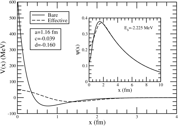
Figure 1: Bare (solid line) and effective (dashed line) $NN$ potentials in a realistic 1-dimensional model. The inset shows “deuteron” ground-state wavefunctions. The sharp features of the bare potential are no longer present in the effective potential. Although the short-distance structure of the wavefunctions are different, the exponential falloff (binding energy) is unchanged.

II.3 Effective Operators

One of the main criticisms levied on traditional shell-model approaches is the lack of consistency between the construction of the effective potential and the renormalization (if any) of the bare operators Hax99 ; Hax01 . While important steps have been taken to correct this inconsistency, both in the area of low-dimensional quantum magnets Pie98b and nuclear structure Nav00b , these are in the very early stages. Further, it is unknown how to construct effective operators that are consistent with both the effective theory and similarity-transformation based approaches.

In this contribution we propose an approach for the modification of operators that is consistent, indeed mimics, the construction of the effective potential. We assume that the momentum dependence of matrix elements of (simple) single-particle operators may be accounted for by an expansion in powers of $k^{2}$ having the same form as the effective-range formula [Eq. (7)]. To do so, one demands that matrix elements of effective operators (${\cal O}_{\rm eff}$) with scattering-wave solutions of the effective potential ($\psi_{k}^{\rm eff}$) possess the same momentum dependence as those using the bare operators with the exact wavefunctions. In analogy with the definition of the effective potential [Eq. (10)], we parametrize the effective operators via

$${\mathcal{O}}_{\rm eff}(x;c,d,\ldots)={\mathcal{O}}(x)\left[1+\left(c+d\frac{\partial^{2}}{\partial\xi^{2}}+\ldots\right)\exp(-\xi^{2})\right]\;.$$ (14)

This parameterization affects only the short-range behavior of the operator just as using the effective potential modifies only the short-range structure of the wavefunction. The parameters $c$, $d$, $\ldots$ (as before) are tuned to the low-$k^{2}$ behavior of the exact matrix elements. To be more specific about our procedure, we fit—in complete analogy to Eq. (13)—the parameters of the effective operator by requiring that

$$\delta\langle{\mathcal{O}}\rangle(k;c,d,\ldots)\equiv\int_{0}^{\infty}dx\Big{(}\psi_{k}(x){\mathcal{O}}(x)\psi_{k\!=\!0}(x)-\psi_{k}^{\rm eff}(x){\mathcal{O}}_{\rm eff}(x;c,d,\ldots)\psi^{\rm eff}_{k\!=\!0}(x)\Big{)}=0\;.$$ (15)

The integral in this expression is convergent as the effective theory demands that

$$\lim_{x\rightarrow\infty}\psi_{k}^{\rm eff}(x)=\psi_{k}(x)\;,$$ (16a)

$$\lim_{x\rightarrow\infty}{\mathcal{O}}_{\rm eff}(x;c,d,\ldots)={\mathcal{O}}(x)\;.$$ (16b)

However, to insure that each term separately is convergent, we add and subtract the following term:

$$\int_{0}^{\infty}dx\Big{(}\phi_{k}(x){\mathcal{O}}(x)\phi_{k\!=\!0}(x)\Big{)}\;,$$ (17)

where we recall that $\phi_{k}(x)$ is the free solution of the 1D scattering problem [see Eq. (2b)].

To extract the parameters of the effective operator we now fit—in the spirit of the effective-range expansion—the low-energy matrix elements of the bare operator between bare scattering wavefunctions according to

$$\langle{\mathcal{O}}\rangle_{\rm BB}(k)=\int_{0}^{\infty}dx\Big{(}\psi_{k}(x){\mathcal{O}}(x)\psi_{k\!=\!0}(x)-\phi_{k}(x){\mathcal{O}}(x)\phi_{k\!=\!0}(x)\Big{)}=\alpha+\beta k^{2}+\ldots$$ (18)

The parameters fixing the effective operators are then adjusted so that the above expansion is recovered. That is,

$$\langle{\mathcal{O}}\rangle_{\rm EE}(k)=\int_{0}^{\infty}dx\Big{(}\psi^{\rm eff}_{k}(x){\mathcal{O}}_{\rm eff}(x;b,c,\dots)\psi^{\rm eff}_{k\!=\!0}(x)-\phi_{k}(x){\mathcal{O}}(x)\phi_{k\!=\!0}(x)\Big{)}=\alpha+\beta k^{2}+\ldots$$ (19)

Note that when ${\mathcal{O}}(x)\!=\!{\mathcal{O}}_{\rm eff}\!=\!1$ one recovers the effective-range expansion.

III Results

In this section we compute matrix elements of various operators using three different schemes. The first scheme uses bare operators with bare wavefunctions (we label these calculations as “B+B”); these should be regarded as “exact” answers. Second, we compute matrix elements in an approximation (labeled as “B+E”) that uses effective wavefunctions but retains bare operators. As we show below, for operators insensitive to short-range physics this inconsistency introduces small discrepancies. However, the more important the short-range physics, the greater the lack of accord. Finally, we perform calculations in a consistent low-energy approximation (“E+E”) that employs both effective wavefunctions and effective operators. Showing that these calculations are in excellent agreement with the exact (B+B) answers represents the central result of the present work.

Because of its simplicity, a natural place to start testing the proposed approach is the calculation of the root-mean-square radius of the deuteron, which is given by

$$\langle{x}^{2}\rangle_{BB}\equiv\Big{\langle}\frac{1}{2}\sum_{n=1}^{2}\Big{(}x_{n}-x_{\rm cm}\Big{)}^{2}\Big{\rangle}=\int_{-\infty}^{\infty}dx\frac{x^{2}}{4}\psi_{\rm gs}^{2}(x)=(1.87977)^{2}~{}{\rm fm}^{2}\;.$$ (20)

The corresponding calculation in the effective theory requires a renormalization of the bare operator. To do so we follow the prescription outlined in the preceding section [see Eqs. (18) and (19)] to obtain

$$x^{2}_{\rm eff}=x^{2}\left[1+\left(c+d\frac{\partial^{2}}{\partial\xi^{2}}\right)\exp(-\xi^{2})\right]\quad(c=1.520,d=-0.305)\;.$$ (21)

In this manner the root-mean-square radius predicted by the effective theory becomes

$$\langle{x}^{2}\rangle_{\rm EE}=\int_{-\infty}^{\infty}dx\frac{x^{2}_{\rm eff}}{4}\Big{(}\psi_{\rm gs}^{\rm eff}(x)\Big{)}^{2}=(1.87988)^{2}~{}{\rm fm}^{2}\;.$$ (22)

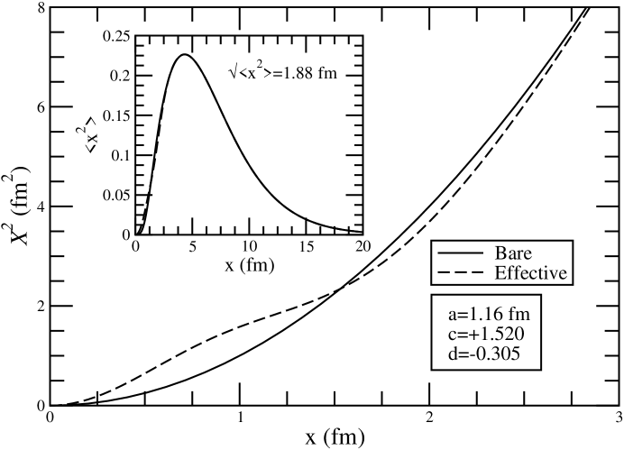
Figure 2: Bare (solid line) and effective (dashed line) $X^{2}$ operator. Note that while the operators are considerably different at short distances, its ground-state expectation values are not (see inset).

This represents a discrepancy of about $1$ part in $10^{4}$. While this result is gratifying and lends some credibiliity to the approach, it hardly qualifies as a stringent test of the formalism. Although both the effective operator and the ground-state wavefunction are modified at short distances (see Fig. 1 and 2) the operator itself has so little support at short distances that the two integrands [Eqs. (20) and (22)] become practically indistinguishable from each other (see inset on Fig. 2). Indeed, an acceptable result is obtained even when the operator is not properly renormalized:

$$\langle{x}^{2}\rangle_{\rm BE}=\int_{-\infty}^{\infty}dx\frac{x^{2}}{4}\Big{(}\psi_{\rm gs}^{\rm eff}(x)\Big{)}^{2}=(1.87834)^{2}~{}{\rm fm}^{2}\;.$$ (23)

A more sensitive test of the approach is provided by the elastic form factor of the deuteron, which in our simple one dimensional model reduces to the following expression:

$$F_{\rm el}(q)=|\rho(q)|^{2}\;,\quad\rho(q)=\int_{-\infty}^{\infty}dx\cos\left(\frac{qx}{2}\right)\psi_{\rm gs}^{2}(x)=1-\frac{q^{2}}{2}\langle{x}^{2}\rangle+{\mathcal{O}}(q^{4})\;.$$ (24)

The corresponding expressions in the B+E and E+E approximations are given by

$$\rho(q)_{\rm BE}=\int_{-\infty}^{\infty}dx\cos\left(\frac{qx}{2}\right)\Big{(}\psi_{\rm gs}^{\rm eff}(x)\Big{)}^{2}\;,$$ (25a)

$$\rho(q)_{\rm EE}=\int_{-\infty}^{\infty}dx\left[\cos\left(\frac{qx}{2}\right)\right]_{\rm eff}\Big{(}\psi_{\rm gs}^{\rm eff}(x)\Big{)}^{2}\;,$$ (25b)

with the effective operator renormalized at short-distances as detailed above. That is,

$$\left[\cos\left(\frac{qx}{2}\right)\right]_{\rm eff}=\cos\left(\frac{qx}{2}\right)\left[1+\left(c(q)+d(q)\frac{\partial^{2}}{\partial\xi^{2}}\right)\exp(-\xi^{2})\right]\;,$$ (26)

The renormalization procedure is illustrated in Fig. 3 at the single momentum-transfer value of $q\!=\!2~{}{\rm fm}^{-1}$. It is important to note that the renormalization coefficients ($c$ and $d$) must be tuned at each value of the momentum transfer $q$. The solid line in the figure displays an effective-range-like expansion for the bare operator ${\mathcal{O}}(x)\!=\!\cos(qx/2)$ [as described in Eq. (18), with the slope and intercept clearly indicated in the figure (note that for clarity the plots are normalized to one at $k^{2}\!=\!0$). It becomes immediately evident that the predicted low-energy behavior of the exact theory can not be reproduced without a proper renormalization of the operator. Indeed, the B+E calculation predicts the wrong momentum dependence; the sign of the slope is wrong! In contrast, it becomes a simple matter to tune the parameters of the effective operator to reproduce exactly the low-energy behavior of the exact theory (dashed line).

Figure 3: An effective-range-like expansion for the elastic form factor of the deuteron at $q\!=\!2~{}{\rm fm}^{-1}$. Calculations are displayed for the bare theory (“B+B”), the effective theory (“E+E”), and for a “hybrid” approximation that uses bare operators with effective wavefunctions (“B+E”). The solid (B+B) and dashed lines (E+E) are identical (by construction) since the effective parameters ($c$ and $d$) are tuned to reproduce the expansion for the bare theory.

Having corrected the short-distance structure of the operator one proceeds to compute the elastic form factor of the deuteron, which now is a prediction of the effective theory. The structure of the form factor (again at $q\!=\!2~{}{\rm fm}^{-1}$) is shown in Fig. 4. The main panel shows bare (i.e., $\cos(x)$) and effective operators, displayed as solid and dashed lines, respectively. Both the effective deuteron wavefunction (inset on Fig. 1) and the effective operator differ considerably from their bare counterparts at short distances—and so is the product of the (square of the) wavefunction times the operator (inset on Fig. 4). Yet the area under the curve—whose square is proportional to the elastic form factor—is essentially unchanged. For comparison, the exact (B+B) and effective (E+E) theories yield values of $F_{\rm el}\!=\!0.02019$ and $F_{\rm el}\!=\!0.02012$, respectively. In contrast, a (B+E) calculation with an effective wavefunction—but still employing a bare operator—results in a discrepancy of nearly 20% ($F_{\rm el}\!=\!0.017062$).

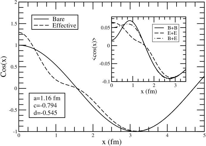
Figure 4: Bare (solid line) and effective (dashed line) for the $\cos(x)$ operator. The inset shows the product of the square of the wavefunction with the operator for the three calculations discussed in the text. The elastic form factor of the deuteron (at $q\!=\!2~{}{\rm fm}^{-1}$) is proportional to the square of the area under the curve.

We conclude the discussion of the elastic form factor of the deuteron by displaying in Fig. 5 its momentum-transfer dependence up to $q\!=\!5~{}{\rm fm}^{-1}$. Recall that effective parameters must be tuned for every value of $q$. It is evident from the figure that the renormalization of the operator at high-momentum transfers is essential, as it is at high $q$ that the short-distance structure of the wavefunction (and of the potential) is being probed. Failing to correct the operator results in a rather poor representation of the elastic form factor for $q\gtrsim 2~{}{\rm fm}^{-1}$ (squares).

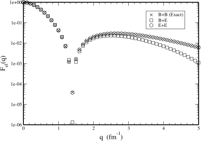
Figure 5: The elastic form factor of the deuteron in the three calculations discussed in the text. Note that the predictions from the effective theory (E+E) agree with the exact theory at at all values of the momentum transfer $q$.

For completeness, and as a further stringent test of the formalism, we compute ground-state observables for an operator with the most extreme short-range structure possible: the Dirac delta function. In the bare theory the ground-state expectation value is simply given by the square of the deuteron wavefunction at the origin. That is,

$$\langle\delta(x)\rangle=\int_{-\infty}^{\infty}dx\delta(x)\psi^{2}_{\rm gs}(x)=\psi^{2}_{\rm gs}(0)=0.01521{\rm fm}^{-1}\;.$$ (27)

As the sharp features of the bare potential are no longer present in the effective potential, the effective deuteron wavefunction at short distances is considerably larger than the bare wavefunction (see Fig. 1). As a result, a (B+E) calculation using an effective wavefunction but a bare delta-function operator grossly overestimates the result: $\langle\delta(x)\rangle_{BE}\!=\!0.04981{\rm fm}^{-1}$. Instead, by following the renormalization procedure outlined above, one obtains an effective Dirac delta-function operator,

$$\delta_{\rm eff}(x)=\frac{1}{a}\left(c+d\frac{\partial^{2}}{\partial\xi^{2}}\right)\exp(-\xi^{2})\quad(c=0.250,d=-0.035)\;,$$ (28)

that yields a ground-state expectation value of $\langle\delta(x)\rangle_{EE}\!=\!0.01523~{}{\rm fm}^{-1}$. This result deviates from the exact value by less than one part in a thousand.

In Table 1 we have listed (for completeness) some of the results presented previously in graphical form. The operators appearing in this table are listed in order of the importance of their short-range components. For example, the root-mean-square radius of the deuteron depends little on the short-range structure of the wavefunction while the Dirac $\delta$-function operator depends exclusively on it. For each operator, we show the two effective coefficients $c$ and $d$ determined by the fitting procedure outlined above. All these are dimensionless quantities and it is gratifying that they are all of order one in keeping with the priciple of “naturalness” Kolck . We note that in some cases failing to renormalize the operator (B+E) leads to discrepancies that are as large as 50% or even 100%. In contrast, calculations using effective wavefunctions and effective operators (E+E) show excellent agreement with B+B calculations regardless of the short-range structure of the operator. We stress that all these are predictions of the effective theory, as the tuning of parameters is done in the scattering sector. In particular, it is satisfying that the elastic form factor of the deuteron at $q\!=\!0$ deviates from unity by less than 2 parts in a thousand. We emphasize that such precise agreement is non-trivial; indeed, it reflects the soundness of our method.

$\langle{\mathcal{O}}(x)\rangle$	$c$	$d$	B+B	B+E	E+E
$\sqrt{<x^{2}>}$	$+1.51979$	$-0.30545$	$1.87997$	$1.87834$ (0.09%)	$1.87988$ (0.01%)
$|\langle\cos(0)\rangle|^{2}$	$-0.02016$	$+0.02985$	$1.00000$	$1.00000$ (0.00%)	$1.00155$ (0.16%)
$|\langle\cos(x/2)\rangle|^{2}$	$-0.06440$	$+0.13429$	$0.04159$	$0.04261$ (2.45%)	$0.04181$ (0.53%)
$|\langle\cos(x)\rangle|^{2}$	$-0.79386$	$-0.54503$	$0.02019$	$0.01706$ (18.4%)	$0.02012$ (0.35%)
$|\langle\cos(2x)\rangle|^{2}$	$-0.52925$	$+0.14806$	$0.01541$	$0.00698$ (220%)	$0.01544$ (0.19%)
$\langle\delta(x)\rangle$	$+0.24964$	$-0.03501$	$0.01521$	$0.04981$ (327%)	$0.01523$ (0.13%)

Table 1: Ground-state expectation values for various operators in the different approximation schemes described in the text. B+B indicates bare operators with bare wavefunctions, B+E bare operators with effective wavefunctions, and E+E effective operators with effective wavefunctions. Note that the root-mean-square radii are given in fm and $\langle\delta(x)\rangle$ in fm^-1. Finally, the $c$ and $d$ coefficients are dimensionless parameters of the effective theory.

IV Conclusions

While the field of nuclear structure has benefited from recent advances in numerical algorithms and sheer computational power, the shell-model problem, in its purest form, remains intractable. As a result, an important part of the nuclear-structure program for many years has focused on the construction of effective interactions for use in shell-model calculations. Two of the most promising approaches are based on the so-called similarity transformation methods (in its many varieties) and on effective-field-theory techniques. The main tenet underlying both approaches is that the short-distance structure of a theory (which is complicated and at present unknown) are hidden to a long-wavelength probe. It should then be possible to “soften” the corresponding short-range portion of the potential while leaving all low-energy properties of the theory intact, thereby providing a significantly more tractible – from a computational point of view – interaction.

The main focus of the present paper is the determination of single-particle operators which can be employed consistently in conjunction with wavefunctions obtained using effective interactions. As observed by many authors, such consistency is essential to the correct implementation of effective theories. For computational simplicity we adopted a one-dimensional $NN$ interaction, that nevertheless incorporates the well-known pathologies of a realistic $NN$ potential. The central result of this work is the proposal and implementation of a single underlying approach for the construction of both effective interactions and effective operators. The construction of the effective interaction follows a well-known approach that is based on a textbook derivation of the effective-range expansion. What is not well known (at least to us) is that the same approach may be generalized to effective operators.

Results from such an implementation are very gratifying, as evinced from a variety of calculations of ground-state observables. For those observables insensitive to the short-range structure of the potential, such as the root-mean-square radius of the deuteron, the renormalization of the bare operator, while required by consistency, is of little numerical consequence. Yet, failing to properly renormalized operators sensitive to short-range physics, such as the elastic form factor of the deuteron at high-momentum transfers, can yield discrepancies as large as 200%. The consistent renormalization procedure advocated here yields in all cases errors of less than 1%.

We conclude with a short comment on future work. The results presented here are encouraging and lend validity to the proposed approach, which is currently being extended to the three-body system. Different algorithms are being employed to solve for the ground-state of the three-body system and in all cases, perhaps not surprisingly, better convergence properties are obtained with the effective rather than with the bare interaction. The results obtained here also constitute a promising first step toward our ultimate goal of combining similarity-transformation methods with effective interactions. The effective interactions and operators obtained here—with their sharp short-range features no longer present—could provide a more suitable starting point for the numerically-intensive approaches based on similarity transformations. Finally, the method proposed here will have to be extended to three-spatial dimensions. Other than numerical complexity, we do not foresee other serious challenges. Indeed, the approach presented here for the construction of effective interactions (whose three-dimensional derivation may be found in several textbooks) had to be adapted to one spatial dimension. In summary, a novel approach for the renormalization of operators in a manner consistent with the construction of the effective potential has been proposed and implemented with considerable success. The results obtained here are gratifying and suggest how in the future effective theories may be profitably combined with more traditional methods to tackle the nuclear many-body problem.

- (1) G.P. Lepage, “How to Renormalize the Schroedinger Equation”, nucl-th/9706029.
- (2) S.R. Beane, P.F. Bedaque, W.C. Haxton, D.R. Phillips and M.J. Savage, nucl-th/0008064.
- (3) P. Navrátil, G.P. Kamuntavičius and B.R. Barrett, Phys. Rev. C 61, 044001 (2000).
- (4) P. Navrátil, J.P. Vary, and B.R. Barrett, Phys. Rev. C 62, 054311 (2000); Phys. Rev. Lett. 84, 5728 (2000).
- (5) M.S. Fayache, J.P. Vary, B.R. Barrett, P. Navratil, and S. Aroua, nucl-th/0112066.
- (6) E.M. Krenciglowa and T.T.S. Kuo, Nuclear Physics A235, 171 (1974).
- (7) K. Suzuki and S.Y. Lee, Prog. Theor. Phys. 64, 2091 (1980).
- (8) K. Suzuki, Prog. Theor. Phys. 68, 246 (1982).
- (9) K. Suzuki and R. Okamoto, Prog. Theor. Phys. 70, 439 (1983).
- (10) W.C. Haxton and C.-L. Song, Phys. Rev.Lett. 84, 5484 (2000); nucl-th/9906082.
- (11) W.C. Haxton and T. Luu, Nucl. Phys. A690, 15 (2001).
- (12) J. Piekarewicz and J.R. Shepard, Phys. Rev. B56, 5366 (1997).
- (13) J. Piekarewicz and J.R. Shepard, Rev. Mex. Fis. 44, 113 (1998).
- (14) J. Piekarewicz and J.R. Shepard, Phys. Rev. B57, 10260 (1998).
- (15) J. Piekarewicz and J.R. Shepard, Phys. Rev. B58, 9326 (1998).
- (16) J. Piekarewicz and J.R. Shepard, Phys. Rev. B60, 9456 (1999).
- (17) H. Mueller, J. Piekarewicz, and J.R. Shepard Phys. Rev.C 66, 024324 (2002).
- (18) C.J. Morningstar and M. Weinstein, Phys. Rev. Lett. 73, 1873 (1994).
- (19) C.J. Morningstar and M. Weinstein, Phys. Rev. D 54, 4131 (1996).
- (20) S.K. Bogner and T.T.S. Kuo, Phys. Lett. B500, 279 (2001)
- (21) M. Birse, J. McGovern and K. Richardson, Phys. Lett. B454, 167 (1999).
- (22) P. Bedaque and U. van Kolck, Ann. Rev. Nucl. Part. Sci 52, 339 (2002).
- (23) T. Barford and M. Birse, hep-ph/0206146.
- (24) L.I.Schiff, Quantum Mechanics (McGraw-Hill, New York, 1968).
- (25) J.R.Taylor, Scattering Theory (John Wiley and Sons, 1972)
- (26) James V. Steele and R.J. Furnstahl, Nucl. Phys. A637, 46 (1998).
- (27) James V. Steele and R.J. Furnstahl, Nucl. Phys. A645, 439 (1999).
- (28) Steven Weinberg, Nucl. Phys. B363, 3 (1991).
- (29) U. van Kolck, L.J. Abu-Raddad and D.M. Cardamone, nucl-th/0205058.