Negative specific heat in a thermodynamic model of multifragmentation

Abstract

We consider a soluble model of multifragmentation which is similar in spirit to many models which have been used to fit intermediate energy heavy ion collision data. In this model $c_{v}$ is always positive but for finite nuclei $c_{p}$ can be negative for some temperatures and pressures. Furthermore, negative values of $c_{p}$ can be obtained in canonical treatment. One does not need to use the microcanonical ensemble. Negative values for $c_{p}$ can persist for systems as large as 200 paticles but this depends upon parameters used in the model calculation. As expected, negative specific heats are absent in the thermodynamic limit.

I Introduction

This paper deals with specific heats of an assembly of interacting nucleons. In recent times the subject has received a great deal of attention [1, 2, 3, 4, 5, 6]. The topic is beset with many controversies. Some of the ideas are : under suitable condtions, nuclear systems exhibit negative heat capacities; negative heat capacities are obtainable only in the microcanonical ensemble; negative heat capacities also appear in canonical models but disappear once the drop size crosses the value $\approx$ 60.

We investigate the specific heats using a thermodynamic model. The basic assumption of the model is that populations of different channels are dictated solely by phase space considerations. This is a common theme in many applications, for example, SMM (statistical multifragmentation model) [1] and MMMC (microcanonical metropolis Monte Carlo) model [2] although details vary from one model to another.

A canonical model based on this assumption was shown to be easily soluble requiring only very quick and simple computing [7]. The first application used one kind of particle but was later extended to two kinds of particles [8, 9]. This appears to be accurate enough for many applications [10] and will undoubtedly be used more and more in the future. We investigate the question of specific heat in this model primarily using one kind of particle. Two kinds of particles were also used but requires longer computing time but we expect no changes from the lessons learnt from the model of one kind of particles. We will however show also some results obtained from using two kinds of particles.

What we will show is that although $c_{v}$ for this model is always positive, $c_{p}$ can sometimes be negative. This is a finite particle number effect and negative values disappear in the thermodynamic limit. Furthermore we get negative values of $c_{p}$ in the canonical model itself. We did not need to go to the microcanonical description. Thermodynamic limit is obtained by using the grand canonical ensemble whereas finite systems are described by canonical model with exact particle number. We find that negative values of $c_{p}$ can persist for fairly large systems although this is dependent upon binding energies used etc.. This was not investigated in detail.

The statements made above appear to hold for the Lattice Gas Model as well. It was demonstrated that $c_{v}$ is positve in the Lattice Gas Model even for a very small system. This can be shown almost analytically without having to use a Monte-Carlo simulation [4] On the other hand $c_{p}$ is much harder to calculate in the Lattice Gas Model. Chomaz et al find that $c_{p}$ can be negative in the Lattics Gas Model [3].

For completeness we describe the canonical thermodynamic model in Section II. In the next section we set up the grand canonical model to get to the thermodynamic limit. Subsequent sections will show the results.

II The Thermodynamic Model

The thermodynamic model has been described in many places [7, 8, 11]. For completeness and to enumerate the parameters we provide some details. We describe the model for one kind of particles only. The generalisation to two kinds could be found in [8, 11].

If there are $A$ identical particles of only one kind in an enclosure at temperature $T$, the partition function of the system can be written as

$$Q_{A}=\frac{1}{A!}(\omega)^{A}$$ (1)

Here $\omega$ is the partition function of one particle. For a spinless particle this is $\omega=\frac{V}{h^{3}}(2\pi mT)^{3/2}$; $m$ is the mass of the particle; $V$ is the available volume within which each particle moves; $A!$ corrects for Gibb’s paradox. If there are many species, the generalisation is

$$Q_{A}=\sum\prod_{i}\frac{(\omega_{i})^{n_{i}}}{n_{i}!}$$ (2)

Here $\omega_{i}$ is the partition function of a composite which has $i$ nucleons. For a dimer $i=2$, for a trimer $i=3$ etc. Equation (2.2) is no longer trivial to calculate. The trouble is with the sum in the right hand side of eq. (2.2). The sum is restrictive. We need to consider only those partitions of the number $A$ which satisfy $A=\sum in_{i}$. The number of partitions which satisfies the sum is enormous when A is large. We can call a given allowed partition to be a channel. The probablity of the occurrence of a given channel $P(\vec{n})\equiv P(n_{1},n_{2},n_{3}....)$ is

$$P(\vec{n})=\frac{1}{Q_{A}}\prod\frac{(\omega_{i})^{n_{i}}}{n_{i}!}$$ (3)

The average number of composites of $i$ nucleons is easily seen from the above equation to be

$$<n_{i}>=\omega_{i}\frac{Q_{A-i}}{Q_{A}}$$ (4)

Since $\sum in_{i}=A$, one readily arrives at a recursion relation [12]

$$Q_{A}=\frac{1}{A}\sum_{k=1}^{k=A}k\omega_{k}Q_{A-k}$$ (5)

For one kind of particle, $Q_{A}$ above is easily evaluated on a computer for $A$ as large as 3000 in matter of seconds. It is this recursion relation that makes the computation so easy in the model. Of course, once one has the partition function all relevant thermodynamic quantities can be computed.

We now need an expression for $\omega_{k}$ which can mimic the nuclear physics situation. We take

$$\omega_{k}=\frac{V}{h^{3}}(2\pi mT)^{3/2}k^{3/2}q_{k}$$ (6)

where the first part arises from the centre of mass motion of the composite which has $k$ nucleons and $q_{k}$ is the internal partition function. For $k=1$, $q_{k}=1$ and for $k\geq 2$ it is taken to be

$$q_{k}=\exp[(W_{0}k-\sigma(T)k^{2/3}+T^{2}k/\epsilon_{0})/T]$$ (7)

Here, as in [1], $W_{0}$=16 MeV is the volume energy term, $\sigma(T)$ is a temperature dependent surface tension term and the last term arises from summing over excited states in the Fermi-gas model. The value of $\epsilon_{0}$ is taken to be 16 MeV. The explicit expression for $\sigma(T)$ used here is $\sigma(T)=\sigma_{0}[(T_{c}^{2}-T^{2})/(T_{c}^{2}+T^{2})]^{5/4}$ with $\sigma_{0}=$18 MeV and $T_{c}=18$ MeV. In the nuclear case one might be tempted to interpret $V$ of eq.(2.6) as simply the freeze-out volume but it is clearly less than that; $V$ is the volume available to the particles for the centre of mass motion. Assume that the only interaction between clusters is that they can not overlap one another. This assumption restricts the validity of the model to low density limit as was stressed in all previous applications of of the model. In the Van der Waals spirit we take $V=V_{freeze}-V_{ex}$ where $V_{ex}$ is taken here to be constant and equal to $V_{0}=A/\rho_{0}$. The precise value of $V_{ex}$ is inconsequential so long as it is taken to be constant. Calculations employ $V$; the value $V_{ex}$ enters only if results are plotted against $\rho/\rho_{0}=V_{0}/(V+V_{ex})$ where $\rho$ is the freeze-out density.

In the past, calculations with one kind of particle used the parametrisation of eq. (2.7) for all $k$’s however large. This means that if the system has $A$ nucleons, the largest possible cluster allowed in the system also has $A$ nucleons. While we will show a few cases with this specification we will also consider a variation. We will take the value of $q_{k}$ to be given by eq. (2.7) up to a limit $k=N$ and zero afterwards. When $A>N$, this simply means that the largest cluster has $N$ nucleons.

Using standard definitions: $E=T^{2}\frac{\partial lnQ_{A}}{\partial T}$ and pressure $p=T\frac{\partial lnQ_{A}}{\partial V}$ we arrive at

$$E=\sum<n_{k}>(E_{k}^{kin}+E_{k}^{int})$$ (8)

where $E_{k}^{kin}=\frac{3}{2}T$ and $E_{k}^{int}=k(-W_{0}+T^{2}/\epsilon_{0})+\sigma(T)k^{2/3}-T[\partial\sigma(T)/\partial T]k^{2/3}$. The last term in $E_{k}^{int}$ was neglected in [7]. It is included here but makes little difference. The expression for pressure is

$$p=\frac{T}{V}\sum<n_{i}>$$ (9)

Multiplicity $m$ is given by $m=\sum<n_{i}>$.

III Infinite matter limit: grand canonical model

If there were only monomers in the grand canonical ensemble one would solve

$$\rho=\exp(\mu/T)\tilde{\omega}_{1}$$ (10)

where $\tilde{\omega}_{i}=\omega_{i}/V$ of section II. Given $\rho$ and $T$ one then finds the chemical potential $\mu$. The number of particles is then given by $A=\rho V$ where $V$ and $A$ are very large (thermodynamic limit). The fluctuations in the number of particles implied by the use of grand canonical ensemble are then negligible compared to the average number $A$.

If we have a model where the only allowed species are monomers and dimers and the total particle number is very large one would solve:

$$\rho=\exp(\mu/T)\tilde{\omega}_{1}+2\times\exp(2\mu/T)\tilde{\omega}_{2}$$ (11)

where phase-space consideration has implied that chemical equilibration exists, that is, the chemical potential of the dimer is twice that of the monomer, i.e., $\mu_{2}=2\mu$.

For a system which is very large but, for which, the heaviest cluster has $N$ nucleons and no more, one needs to solve

$$\rho=\sum_{1}^{N}k\exp(k\mu/T)\tilde{\omega}_{k}$$ (12)

In this case, one might argue that one is considering a model in which the composites obey eq.(2.6) up to $k=N$ and $\omega_{k}$’s for $k>N$ are all zeroes. Of course it is possible that both $A$ and $N$ are very large. Use of the grand canonical ensemble always implies that $A$ is very large but $N$ may be large or small.

Pressure in the grand canonical model is calculated from $p=(T/V)lnZ_{grand}$ which in this model reduces to $p=(T/V)\sum<n_{i}>$ where $<n_{i}>/V=\exp(i\mu/T)\tilde{\omega}_{i}$. Notice that formally this eq. is same as eq.(2.9) but, of course, $<n_{i}>$ in eq. (2.9) is calculated according to the canonical formula, eq.(2.4).

IV specific heats in the model

In [7] where the canonical thermodynamic model was first studied for phase transitions, it was pointed out that for a given density $\rho$, the specific heat per particle $c_{v}=C_{V}/A$ tends to $\infty$ at a particular temperature when the particle number $A$ tends to $\infty$. Since,

$C_{V}=\left(\frac{\partial E}{\partial T}\right)_{V}=T\left(\frac{\partial S}{\partial T}\right)_{V}=-T\left(\frac{\partial^{2}F}{\partial^{2}T}\right)_{V},$

a singularity in $C_{V}$ signifies a break in the first derivative of $F$, the free energy and a first order phase transition. The specific heat $c_{v}$ in the model has been studied in more than one application and always found to be positive. We now turn our attention to $c_{p}$ studied in this canonical model. It is instructive to look at $p-\rho$ curves at different temperatures (equation of state) to gain an understanding (Fig.1). For 200 particles ($A$=200 and $N$=number of nucleons of the largest allowed cluster=200) this is drawn at three temperatures: $T_{1}<T_{2}<T_{3}$. Here $T_{2}$ is only slightly higher than $T_{1}$. We notice that on $T_{1},T_{2}$ isothermals there are regions of mechanical instability where $\partial p/\partial\rho$ is negative. It is in this region that one encounters negative values for $c_{p}$. Instead of $\rho$ let us use the variable $V\propto 1/\rho$. Thus regions of mechanical instability are characterised by $\partial p/\partial V>$0. Let us try to understand how this can happen. In simpler cases as in a gas of noninteracting monomers, the multiplicity $m$ (which determines the pressure, i.e., $p=T\times\frac{m}{V})$ is simply $A$ and $(\partial p/\partial V)_{T}$ is always negative. (we actually use $m-1$ rather than $m$ for calculating $p$ but this is immaterial for our discussion). In the thermodynamic model, because of composites, $m<<A$ at moderate temperatures. At fixed temperature $T>0$, $m$ will always increase with $V$. Negative compressibility is marked by $(\frac{\partial m}{\partial V})_{T}>\frac{m}{V}$. Let us consider points $a,b$ (region of positive $c_{p}$) and points $c,d$ (region of negative $c_{p}$). Points $b,c$ are on $T_{1}\equiv T$ and points $a,d$ are on $T_{2}\equiv T+\delta T$ with $\delta T>0$. Using

$p=T\frac{m}{V}=(T+\delta T)\frac{m+\delta m}{V+\delta V}$ we arrive at

$$\frac{\delta m}{m}=\frac{\delta V}{V}-\frac{\delta T}{T}$$ (13)

In the region $(c,d)$, $\delta V$ is negative, $\delta T$ ia always positive thus $\delta m$ is negative. If $m$ goes down then so does the kinetic energy and also the potential energy (creating more $m$ creates more surface and hence more energy). Thus in this region with increasing temperature but constant pressure, both the kinetic and the potential energy of the system go down. In the “normal” region $\delta m$ is positive and both the kinetic and the potential energies increase with $T$ at constant pressure. This is illustrared in Table 1. Finally we show, in fig. 2, the caloric curve for a given pressure where in part of the curve temperature does go down with excitation energy. The fall is very gentle whereas the rise with energy when it happens is faster.

The occurrence of a negative $C_{p}$ in spite of a positive $C_{V}$ is allowed in the following well-known relation [17]:

$C_{p}-C_{V}=VT\frac{\alpha^{2}}{\kappa}$

where $\alpha$ is the volume coefficient expansion and $\kappa$ is the isothermal compressibility given by:

$$\alpha = \frac{1}{V}\left(\frac{\partial V}{\partial T}\right)_{p}$$ (14)

$$\kappa = -\frac{1}{V}\left(\frac{\partial V}{\partial p}\right)_{T}.$$ (15)

For negative $\kappa$, $C_{p}$ is less than $C_{V}$ and can become negative.

Using the equality,

$\left(\frac{\partial V}{\partial T}\right)_{p}=-\left(\frac{\partial V}{\partial p}\right)_{T}\left(\frac{\partial p}{\partial T}\right)_{p}$

we can also write,

$C_{p}-C_{V}=VT\left(\frac{\partial p}{\partial T}\right)_{V}\frac{1}{V}\left(\frac{\partial V}{\partial T}\right)_{p}.$

This shows that, $C_{p}$ can drop below $C_{V}$ if isobaric volume coefficient of expansion becomes negative which is the case in some regions of Fig.1.

V Extrapolation to thermodynamic limit

For $A$ very large but N=200 we use the grand canonical ensemble. For a given $\rho$ and $T$, we solve for $\mu$ where $N$ in eq. (3.3) is set at 200. In the $p-\rho$ diagram there are no regions of mechanical instability (see fig. 3). For comparison, the $p-\rho$ diagram for $N=200$ but $A$=200 obtained by the canonical calculation is also shown in the same figure. We see that in the low density side (the gas phase) the two diagrams coincide. The rise of pressure with density is quite rapid and linear. After the two diagrams separate, the rise of pressure with density in the grand canonical model slows down considerably but there is no region of mechanical instability although the canonical calculation with 200 particles has a region of instability. In the grand canonical result which represents the thermodynamic extrapolation, we have not reached the classic liquid-gas coexistence limit where there would be no rise of pressure at all (like in Maxwell construction). We think the reason is this. The largest cluster has size 200 which is not a big enough number. Condensation into the largest and larger clusters still does not behave like a liquid. We now increase the largest cluster size to 2000. Now the coexistence region is very clear and there is unmistakable signature of first order phase transition. This grand canonical result is very close to the case where $N=\infty$ ( see Fig. 3 in [13]). In the same figure we also show results of a canonical calculation with $A$=2000 and $N$=2000. The region of mechanical instability has gone down considerably but it has not disappeared showing that we have not reached the thermodynamic limit yet.

VI More calculations in the canonical model

The mechanical instability which led to negative values of $c_{p}$ is not only a finite number effect but it is also dependent on details of parameters; see also [6]. As in fig.3 we draw a $p-\rho$ diagram for 200 particles in fig. 4 but now the largest cluster has $N=100$, that is, $\omega_{k}$ is given by eq. (2.6) up to $k$=100 and is zero for $k>100$. The mechanical instability region has completely disappeared. In fact, the negative compressility in the $p-\rho$ diagram in fig. 4 disappears even with the following minimal change. We use $q_{k}$ of eq. (2.7) upto $k=100$ and for $k>100$ use $q_{k}=\exp[0.97(W_{0}k-\sigma(T)k^{2/3}+T^{2}k/\epsilon_{0})/T]$. We were surprised that with such small changes zones of negative compressibility disappeared but such consequences were anticipated in other models before [6].

VII Chemical Potentials

In this section we deal with two kinds of particles and discuss the behaviours of chemical potentials as the proton fraction of large systems changes. This is remotely connected with specific heats but the behaviour of chemical potentials with the proton fraction has attracted some attention in recent times and we felt that it is of general interest to show what the behaviour is in the themodynamic model. It was shown that in mean-field theories of nuclear matter there is chemical instability as a function of $y=Z/(N+Z)$ in limited regions of $y$, that is, $({\partial\mu_{P}}/{\partial y})_{p,T}$ becomes negative in some region of $\mu_{P}-y$ plane (correspondingly $({\partial\mu_{N}}/{\partial y})_{p,T}$ becomes positive). This is analgous to mechanical instability as a function of density [14, 15, 16]. We have seen that in the thermodynamic model there are no regions of mechanical instability for large systems (the grand canonical results). We will see that there is no chemical instability either in the model in the large particle number limit. Now we need to consider the thermodynamic model for two kinds of particles. For details we refer to [8]. A composite has two indices: $i$=proton number, $j$=neutron number with $a=i+j$. Analogous to eq.(2.4) we have

$$<n_{i,j}>=\omega_{i,j}\frac{Q_{Z-i,N-j}}{Q_{Z,N}}$$ (16)

where the nuclear properties are contained in $\omega_{i,j}$:

$$\omega_{i,j}=\frac{V}{h^{3}}(2\pi mT)^{3/2}a^{3/2}q_{i,j}$$ (17)

We take the internal partition function of the composite to be

$$q_{i,j}=\exp[(Wa-\sigma a^{2/3}-s\frac{(i-j)^{2}}{a}+aT^{2}/\epsilon_{0})/T]$$ (18)

As is usual in all infinite matter case calculations, the coulomb interaction is switched off. We take $W=15.8$ MeV, $\sigma=18$ MeV,$s$=23.5 MeV and $\epsilon_{0}$=16.0 MeV. For $a\geq 5$ we use this formula. For lower masses we simulate the no coulomb case by setting the binding energy of ³He=binding energy of ³H and binding energy of ⁴Li=binding energy of ⁴H.

For a given $a$ what are the limits on $i$(or $j=a-i$)? This is a non-trivial question. In the results we will show, we have taken the limits by calculating the drip lines of protons and neutrons as given by the binding energy formula. Limiting oneself to within the drip lines is a well-defined prescription, but is likely to be an underestimation since resonances show up in particle-particle correlation experiments. On the other hand, for a given $a$, taking limits of $i$ from 0 to $a$ is definitely an overestimation.

In fig. 5 we have drawn isothermals (at $T$=6.0 MeV) for two component nuclear systems for different $y$’s in the grand canonical ensemble. We restrict $y$ between 0.3 and 0.5 and $\rho/\rho_{0}$ between 0 and 0.5, the ranges for which the thermodynamic model is expected to be reliable. In the calculation the largest cluster is taken to be $a=500$. The same figure also shows the behaviours of $\mu_{P}$ and $\mu_{N}$ at constant pressure. The derivative $\frac{\partial\mu_{p}}{\partial y}$ is seen to be always positive (simultaneously $\frac{\partial\mu_{N}}{\partial y}$ is negative). In the next figure, for completeness, we have continued the model beyond $\rho/\rho_{0}$=0.5 and gone upto the highest possible limit of $\rho/\rho_{0}=1$ in the model to see the behaviour of $\mu_{P}$ and $\mu_{N}$. No chemical instability is seen.

VIII Summary and Discussion

We have shown that with usual concepts one can obtain a negative value of $C_{P}$ in part of the $T-E$ plane within the framework of a thermodynamic model. Although we have shown this, for the sake of simplicity, using one kind of particle only, we have checked that the phenomenon remains when a more complicated version with two kinds of particles and realistic binding energies for the composites are used. The $C_{V}$ is positive and its origin is the cost in surface energy to break large clusters into smaller clusters and nucleons. A negative $C_{p}$ is seen in our exactly soluble canonical ensemble model for small systems. This negative value arises in regions of mechanical instability where the isothermal compressiblity is negative or equivalently, the isobaric volume expansion coefficient is negative. A negative isobaric volume expansion leads to a decrease in multiplicity, or total number of clusters, with temperature and a corresponding decrease in energy. For larger systems these regions disappear and in the grand canonical limit, $C_{p}$ is always positive.

Since several papers have demonstrated the existence of negative specific heats it is pertinent to mention the relevance of our work to these earlier works. Our model is not, in any simple way, connected to negative specific heat found in ten dimensional Potts Model [2]. The specific heat considered in that work is $C_{V}$ and the negative specific heat appears only in microcanonical treatment. The negative specific heat seen here is at least partially similar to that seen in [3, 4]. There is no negative specific heat in $C_{V}$ [4] but it makes its presence felt when $C_{P}$ is considered [3]. Although our model is quite different from the one considered in [6] the results are similar.

Unfortunately we can not recommend any experiments to verify the conclusions of this paper. Nuclear disasembly in heavy ion collisions can not be fine tuned. There is no reason to think that it takes place exactly at constant volume or exactly at constant pressure. Calculations at constant volume gives quite reasonable predictions for observables that have been measured [10, 18] but this does not rule out the possibility that variations happen. If disassembly always took place at constant pressure then the following idealised experiment would be useful. One measures excitation energy per particle and also the temperature. One would then find there are cases where the average excitation energy per particle goes down even though the temperature rises.

IX Acknowledgment

S. Das Gupta acknowledges very useful discussions with Rajat K. Bhaduri, Lee Sobotka and Abhijit Majumder. This work is supported in part by the Natural Sciences and Engineering Research Council of Canada and the U.S. Department of Energy Grant No. DE FG02-96ER40987.

TABLE I.: Variation of energies per particle $(MeV)$ with temperature $(MeV)$ in the negative and positive compressibility zones, for $p=0.017\ MeV\ fm^{-3}$

	$T$	$\rho/\rho_{0}$	$e_{k}/A$	$e_{pot}/A$	$e_{tot}/A$
	6.0	0.146	0.978	-5.235	-4.257
$\frac{\partial p}{\partial\rho}<0$	6.1	0.212	0.638	-6.970	-6.332
	6.2	0.392	0.294	-8.708	-8.414
	6.0	0.104	1.422	-3.271	-1.849
$\frac{\partial p}{\partial\rho}>0$	6.1	0.090	1.653	-2.513	-0.859
	6.2	0.082	1.824	-2.027	-0.202

FIG. 1.: EOS in the canonical model for a system of $A$=200. The largest cluster also has $N$=200.

FIG. 2.: Caloric curve at a constant pressure $(p=0.017\ MeV\ fm^{-3})$ in the canonical model with $A$=200 and $N$=200. The solid and dashed portions of the curve give -ve and +ve $c_{p}$ respectively.

FIG. 3.: EOS at $T=6\ MeV$ in the two models. For the left panel the largest cluster has $N$=200 and for the right panel $N$=2000. For the canonical calculation, the left and right panel has $A$=200 and 2000 respectively, but for the grandcaonocal calculations, $A=\infty$. (See text).

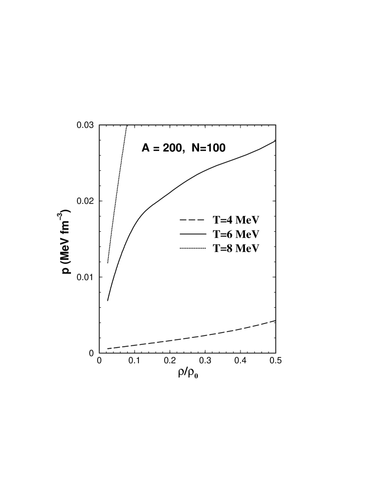
FIG. 4.: EOS in the canonical model for a system of 200 particles, but the number of nucleons of the largest cluster is restricted to 100.

FIG. 5.: The top panel are isothermals at $T=6MeV$ for different $y$’s (proton fraction). The lower panels show the behavior of $\mu_{N}$ and $\mu_{P}$ as a function of $y$ in the density range of the top panel. Calculations are done in a grandcanonical model with the largest cluster having 500 nucleons.

FIG. 6.: The behaviors of $\mu_{N}$ and $\mu_{P}$ extrapolated to higher densities. For this figure the $p-{\rho/\rho_{0}}$ diagram (upper panel Fig.5) was extended upto $\rho/\rho_{0}$=1.

REFERENCES

- [1] J. P. Bondorf, A. S. Botvina, A. S. Iljinov, I. N. Mishustin, and K. Sneppen, Phys. Rep. 257, 133 (1995)
- [2] D. H. E. Gross, Phys. Rep. 279, 119 (1997)
- [3] P. Chomaz, V. Duflot and F. Gulminelli, Phys. Rev. Lett. 85, 3587 (2000)
- [4] C. B. Das and S. Das Gupta, Phys. Rev. C64, 017601 (2001)
- [5] M. D’Agostino et al Nucl. Phys. A699, 795 (2002)
- [6] L. G. Moretto, J. B. Elliott, L. Phair, and G. J. Wozniak, Phys. Rev. C66, 041601 (R) (2002)
- [7] S. Das Gupta and A. Z. Mekjian, Phys. Rev C57, 1361 (1998)
- [8] P. Bhattacharyya, S. Das Gupta and A. Z. Mekjian, Phys. Rev C60, 054616 (1999)
- [9] P. Bhattacharyya, S. Das Gupta and A. Z. Mekjian, Phys. Rev C60, 064625 (1999)
- [10] M. B. Tsang et al, Phys. Rev. C64, 054615 (2001)
- [11] S. Das Gupta, A. Z. Mekjian and M. B. Tsang, Advances in Nuclear Physics, vol.26, 91 (2001)
- [12] K. C. Chase and A. Z. Mekjian, Phys. Rev C50, 2078 (1994)
- [13] K. A. Bugaev, M. I. Gorenstein, I. N. Mishustin and W. Greiner, Phys. Rev C62, 044320 (2000)
- [14] H. Muller and B. D. Serot, Phys. Rev. C52, 2072 (1995)
- [15] H. Muller and B. D. serot, Isospin Physics in Heavy-Ion Collisions at Intermediate Energy, edited by B.A. Li and W. U. Schroder (Nova Science Publishers, Inc.,Huntington, New York, 2001)
- [16] S.J.Lee and A.Z.Mekjian, Phys. Rev. C63, 044605 (2001)).
- [17] F. Reif, Fundamentals of statistical and thermal physics (McGraw-Hill, New York, 1965), ch.8.
- [18] A. Majumder and S. Das Gupta, Phys. Rev. C61, 034603 (2000).