Application of the Adiabatic Selfconsistent-Collective-Coordinate Method
to a Solvable Model of Prolate-Oblate Shape Coexistence

Abstract

The adiabatic selfconsistent collective coordinate method is applied to an exactly solvable multi-$O(4)$ model which simulates nuclear shape coexistence phenomena. Collective mass and dynamics of large amplitude collective motions in this model system are analysed, and it is shown that the method can well describe the tunneling motions through the barrier between the prolate and oblate local minima in the collective potential. Emergence of the doublet pattern is well reproduced.

1 Introduction

Microscopic description of large amplitude collective motion in nuclei is a long-standing fundamental subject of nuclear structure physics [1, 2]. In spite of the steady development in various theoretical concepts and mathematical formulations of them, application of the microscopic many-body theory to actual nuclear phenomena still remains as a challenging subject^3)-30) (see Ref. rf:31 for a recent comprehensive review). Shape coexistence phenomena are typical examples of the nuclear large amplitude collective motion and have been investigated from various points of view^32)-45) For instance, even in typical spherical nuclei like Pb and Sn isotopes, excited deformed states have been systematically observed in low-energy regions[32], and the coexistence of prolate, spherical and oblate shapes have been recently reported for ^186,188Pb[38]. As another example, we mention a recent discovery of coexisting two rotational bands in ⁶⁸Se, which are associated with oblate and prolate intrinsic shapes[39]. These are only a few examples among abundant experimental data. Clearly, these data strongly calls for further development of the theory which is able to describe them and renews our concepts of nuclear structure. From the viewpoint of the microscopic mean-field theory, these phenomena imply that different solutions of the Hartree-Fock-Bogoliubov (HFB) equations (local minima in the deformation energy surface) appear in the same energy region and the nucleus undergoes a large amplitude collective motions connecting these different equilibrium points. Identities or mixings of these different shapes are determined by the dynamics of such collective motions.

On the basis of the time-dependent Hartree-Fock (TDHF) theory, the selfconsistent collective coordinate (SCC) method was proposed as a microscopic theory of such large amplitude collective motions [9]. It was extended to the case of time-dependent HFB (TDHFB) including the pairing correlations[20], and has been successfully applied to various kinds of anharmonic vibration and high-spin rotations^46)-57) In order to apply this method to shape coexistence phenomena, however, we need to further develop the theory, since the known method of solving the basic equations of the SCC method, called $\eta$-expansion method[9], assumes a single local minima whereas several local minima of the potential energy surface compete in these phenomena. Quite recently, a new method of solving the basic equations of the SCC method, called adiabatic SCC (ASCC) method, has been proposed[58]. This new method uses an expansion in terms of the collective momentum and do not assume a single local minima, so that it is expected to be suitable for a description of the shape coexistence phenomena. The ASCC method may also be regarded as a successor of the adiabatic TDHF (ATDHF) methods. It inherits the major achievements of the ATDHF theory (as reviewed in Ref. rf:31) and, in addition, enables us to include the pairing correlations selfconsistently removing the spurious number fluctuation modes.

The major purpose of this paper is to examine the feasibility of the ASCC method for applications to actual nuclear phenomena. This is done by applying it to an exactly solvable model called multi-$O(4)$ model and testing results of the ASCC method against exact solutions obtained by diagonalizating the Hamiltonian in a huge bases. This solvable model may be regarded as a simplified version of the well-known pairing-plus-quadrupole (P+Q) interaction model [59, 60]. Namely, only the $K=0$ component of the quadrupole deformation is considered in a schematic manner, and the model has been widely used as a testing ground for various microscopic theories of nuclear collective motion[61, 62, 63, 64]. The multi-$O(4)$ model possesses a symmetry, analogous to the ordinary parity quantum number, with respect to the sign change of the “quadrupole” deformation. Accordingly, it can be utilized as a simple model of many-body systems possessing double well structure where large amplitude tunneling motions take place through the barrier between the two degenerate local minima of the potential (which correspond to the prolate and oblate shapes). Because of the special symmetry of the model, the “prolate” and “oblate” shapes mix completely. Of course, in contrast to the ordinary parity, such an exact prolate-oblate symmetry does not occur in reality, and in this sense this solvable model is somewhat unrealistic. Nevertheless, using this model, we can make a severe test of the theory by examining its ability to describe the “parity doublet” pattern.

In this paper, we would like to focus our attention on the collective dynamics and the collective mass of large amplitude collective motions. Needless to say, the barrier penetration depends on the collective mass in a quite sensitive manner. A similar investigation on the collective dynamics of this model was done in Ref. rf:27, in which the number fluctuation’s degree of freedom was explicitly removed from the model space. In the present approach, the spurious number fluctuation modes are automatically decoupled from the physical modes within a selfconsistent framework of the TDHFB theory. This will be a great advantage when the method is applied to realistic nuclear problems.

This paper is arranged as follows: In $\S$ 2, the basic equations of the ASCC method are recapitulated. In $\S$ 3, a brief account of the multi-$O(4)$ model is given. In $\S$ 4, we apply the ASCC method to the multi-$O(4)$ model and derive explicit expressions necessary for numerical calculations. In $\S$ 5, we present results of numerical analysis, and conclusions are given in $\S$ 6.

2 Basic equations of the ASCC method

In this section, instead of recapitulating the general outline of the SCC method, we summarize the adiabatic version of them formulated in Ref. rf:58. We assume that large-amplitude collective motions are described by a set of the TDHFB state vectors $\left|\phi(q,p,\varphi,N)\right\rangle$ that are parametrized by a single collective coordinate $q$, the collective momentum $p$ conjugate to $q$, the particle number $N$ and the gauge angle $\varphi$ conjugate to $N$. The time evolution of $\left|\phi(q,p,\varphi,N)\right\rangle$ is determined by the time-dependent variational principle

$$\delta\left\langle\phi(q,p,\varphi,N)\right|i\frac{\partial}{\partial t}-{\hat{H}}\left|\phi(q,p,\varphi,N)\right\rangle=0.$$ (1)

As discussed in Ref. rf:58, we can set

$$\left|\phi(q,p,\varphi,N)\right\rangle=e^{-i\varphi\hat{N}}\left|\phi(q,p,N)\right\rangle.$$ (2)

Then, since the Hamiltonian $\hat{H}$ commutes with the number operator $\hat{N}$, the gauge angle $\varphi$ becomes cyclic. The basic equation of the SCC method consists of the invariant principle of the TDHFB equations (1) and the canonical variable condition which can be written as equations for the state vectors $\left|\phi(q,p,N)\right\rangle$,

$$\left\langle\phi(q,p,N)\right|i{\partial\over\partial q}\left|\phi(q,p,N)\right\rangle =p,$$ (3a)

$$\left\langle\phi(q,p,N)\right|{\partial\over i\partial p}\left|\phi(q,p,N)\right\rangle =0,$$ (3b)

$$\left\langle\phi(q,p,N)\right|\hat{N}\left|\phi(q,p,N)\right\rangle =N,$$ (3c)

$$\left\langle\phi(q,p,N)\right|{\partial\over i\partial N}\left|\phi(q,p,N)\right\rangle =0.$$ (3d)

The third equation guarantees that the particle-number expectation value is kept constant during the large-amplitude collective motion described by the collective variables $(q,p)$. Assuming that the large-amplitude collective motion described by the collective variables $(q,p)$ is slow, we now introduce the adiabatic approximation to the SCC method. Namely we expand the basic equations with respect to the collective momentum $p$. Since the particle-number variable $N$ is a momentum variable in the present formulation, we also expand the basic equations with respect to $n=N-N_{0}$, when we consider a system with particle number $N_{0}$. We then keep only the lowest order term. The TDHFB state vectors are thus written as

$$|\phi(q,p,N)\rangle=e^{ip{\hat{Q}(q)}+in{\hat{\Theta}(q)}}|\phi(q)\rangle,$$ (4)

where $\hat{Q}(q)$ and $\hat{\Theta}(q)$ are infinitesimal generators with respect to $\left|\phi(q)\right\rangle$. We also define an infinitesimal generator $\hat{P}(q)$ by

$$e^{-i\delta q{\hat{P}(q)}}|\phi(q)\rangle=|\phi(q+\delta q)\rangle.$$ (5)

We insert the TDHFB state vectors (4) into (1) and make an expansion with respect to $p$ and $n$. Requiring that the time-dependent variational principle (the canonical variable condition) be fulfilled up to the second (first) order, we obtain the basic set of equations of the ASCC method to determine the infinitesimal generators $\hat{Q}(q)$ and $\hat{P}(q)$ as follows:

Canonical variable conditions

$$\left\langle\phi(q)\right|[\hat{Q}(q),\hat{P}(q)]\left|\phi(q)\right\rangle=i,$$ (6a)

$$\left\langle\phi(q)\right|[\hat{\Theta}(q),\hat{N}]\left|\phi(q)\right\rangle=i,$$ (6b)

the other expectation values of commutators among $\{\hat{Q}(q),\hat{P}(q),\hat{\Theta}(q),\hat{N}\}$ being zero.

HFB equation in the moving frame

$$\delta\left\langle\phi(q)\right|\hat{H}_{M}(q)\left|\phi(q)\right\rangle=0,$$ (7)

where the $\hat{H}_{M}(q)$ is the Hamiltonian in the moving frame defined by

$$\hat{H}_{M}(q)=\hat{H}-\lambda(q)\hat{N}-\frac{\partial V}{\partial q}\hat{Q}(q).$$ (8)

Local harmonic equations

$$\delta\left\langle\phi(q)\right|[\hat{H}_{M}(q),\hat{Q}(q)]-{1\over i}B(q)\hat{P}(q)\left|\phi(q)\right\rangle=0,$$ (9a)

$$\delta\left\langle\phi(q)\right|[\hat{H}_{M}(q),{1\over i}\hat{P}(q)]-C(q)\hat{Q}(q)\\ \\ -{1\over 2B(q)}[[\hat{H}_{M}(q),(\hat{H}-\lambda(q)\hat{N})_{A}],\hat{Q}(q)]-{\partial\lambda\over\partial q}\hat{N}\left|\phi(q)\right\rangle=0,$$ (9b)

where the local stiffness $C(q)$ is defined by

$$C(q)={\partial^{2}V\over\partial q^{2}}+{1\over 2B(q)}{\partial B\over\partial q}{\partial V\over\partial q},$$ (10)

and $(\hat{H}-\lambda\hat{N})_{A}$ indicates the $a^{\dagger}a^{\dagger}$ and $aa$ parts of ($\hat{H}-\lambda\hat{N}$) containing two-quasiparticle creation and annihilation operators. The collective potential $V(q)$, the inverse mass $B(q)$, and the chemical potential $\lambda(q)$ are defined below. Equations (9a) and (9b) are linear equations with respect to the one-body operators $\hat{Q}(q)$ and $\hat{P}(q)$. They have essentially the same structure as the standard RPA equations except for the last two terms in Eq. (9b), which arise from the curvature term (derivative of the generator) and the particle-number constraint, respectively. The infinitesimal generators $\hat{Q}(q)$ and $\hat{P}(q)$ are thus closely related to the harmonic normal modes locally defined for $\left|\phi(q)\right\rangle$ and the moving frame Hamiltonian $\hat{H}_{M}(q)$. The collective subspace defined by these equations will be uniquely determined once a suitable boundary condition is specified.

The collective Hamiltonian is given by

$${\cal H}(q,p,N) \equiv \left\langle\phi(q,p,N)\right|\hat{H}\left|\phi(q,p,N)\right\rangle$$ (11a)

$$= V(q)+{1\over 2}B(q)p^{2}+\lambda(q)n,$$ (11b)

up to the second order in $p$ and the first order in $n$, where

$$V(q) = {\cal H}(q,p,N)|_{p=0,N=N_{0}}=\left\langle\phi(q)\right|\hat{H}\left|\phi(q)\right\rangle,$$ (12)

$$B(q) = {1\over 2}{\partial^{2}{\cal H}(q,p,N)\over\partial p^{2}}|_{p=0,N=N_{0}}=-\left\langle\phi(q)\right|[[\hat{H},\hat{Q}(q)],\hat{Q}(q)]\left|\phi(q)\right\rangle,$$ (13)

$$\lambda(q) = {\partial{\cal H}(q,p,N)\over\partial N}|_{p=0,N=N_{0}}=\left\langle\phi(q)\right|[\hat{H},i\hat{\Theta}(q)]\left|\phi(q)\right\rangle.$$ (14)

For the system with $N=N_{0}$ particles, we can put $n=0$.

3 Multi-$O(4)$ model

The multi-$O(4)$ model may be regarded as a simplified version of the conventional P+Q interaction model[59, 60], where only the $K=0$ component of the quadrupole deformation is considered in a schematic manner. It has been used for schematic analysis of anharmonic vibrations in transitional nuclei and of various kinds of large-amplitude collective motion[61, 62, 63, 64].

We define bilinear fermion operators for each $j$-shell,

$$A_{j}^{\dagger} = \sum_{m>0}c_{jm}^{{\dagger}}c_{j-m}^{{\dagger}},~{}~{}B_{j}^{\dagger}=\sum_{m>0}{\sigma_{jm}}c_{jm}^{{\dagger}}c_{j-m}^{{\dagger}},~{}$$ (15a)

$$\hat{N}_{j} = \sum_{m}c_{jm}^{{\dagger}}c_{jm},~{}~{}~{}~{}~{}\hat{D}_{j}=\sum_{m}{\sigma_{jm}}c_{jm}^{{\dagger}}c_{jm},$$ (15b)

with

$${\sigma_{jm}}=\left\{\begin{array}[]{cc}1&|m|<\Omega_{j}/2\\ -1&|m|>\Omega_{j}/2.\end{array}\right.$$ (16)

The sign of $\sigma_{jm}$ is chosen so as to simulate the behavior of the quadrupole matrix elements $\left\langle jm\right|r^{2}Y_{20}\left|jm\right\rangle$, and we assume that the pair multiplicity $\Omega_{j}=j+\frac{1}{2}$ is an even integer. The set of operators $\{A_{j}^{\dagger},A_{j},B_{j}^{\dagger},B_{j},\hat{N}_{j},\hat{D}_{j}\}$ form a Lie algebra of $O(4)$. We then define their extensions to the multi $j$-shell case,

$$A^{\dagger}=\sum_{j}A^{\dagger}_{j},~{}B^{\dagger}=\sum_{j}B^{\dagger}_{j},~{}\hat{N}=\sum_{j}\hat{N}_{j},~{}\hat{D}=\sum_{j}d_{j}\hat{D}_{j},~{}$$ (17)

the coefficients $d_{j}$ in $\hat{D}$ simulating the magnitudes of the reduced quadrupole matrix elements of the $j$-shells, and introduce a model Hamiltonian

$$\hat{H} = \hat{h}_{0}-\frac{1}{2}G(A^{{\dagger}}A+AA^{{\dagger}})-\frac{1}{2}\chi{\hat{D}}^{2},$$ (18a)

$$\hat{h}_{0} = \sum_{j}e^{0}_{j}{\hat{N}}_{j},$$ (18b)

where $e^{0}_{j}$ denote single-particle energies of the $j$-shells, and $G$ and $\chi$ represent the strengths of the pairing and the “quadrupole” interactions, respectively. Note that this Hamiltonian is invariant with respect to the conversion of single-particle states $(j,\pm|m|)\leftrightarrow(j,\pm(\Omega_{j}-|m|))$. Thus, eigenstates can be classified according to the “parity” quantum number associated with this symmetry.

If we make different combinations of these operators as

$$K_{j+} = \frac{1}{2}(A_{j}^{\dagger}+B_{j}^{\dagger}),~{}~{}~{}~{}~{}~{}~{}~{}~{}L_{j+}=\frac{1}{2}(A_{j}^{\dagger}-B_{j}^{\dagger}),~{}~{}$$ (19a)

$$K_{j-} = \frac{1}{2}(A_{j}+B_{j}),~{}~{}~{}~{}~{}~{}~{}~{}~{}L_{j-}=\frac{1}{2}(A_{j}-B_{j}),~{}~{}$$ (19b)

$$K_{j0} = \frac{1}{2}(\hat{N}_{j}+\hat{D}_{j}-\Omega_{j}),~{}~{}L_{j0}=\frac{1}{2}(\hat{N}_{j}-\hat{D}_{j}-\Omega_{j}),$$ (19c)

the sets $(K_{j+},K_{j-},K_{j0})$ and $(L_{j+},L_{j-},L_{j0})$ separately form $SU(2)$ algebras, and they commute with each other. Namely, the multi-$O(4)$ model is equivalent to the multi $SU(2)\otimes SU(2)$ model. Thus, we can diagonalize the Hamiltonian (18) in a basis set

$$\prod_{j}|n_{Kj},n_{Lj}\rangle=\prod_{j}(K_{j+})^{n_{Kj}}(L_{j+})^{n_{Lj}}|0\rangle,$$ (20)

to get the exact eigenvalues and eigen-vectors, where $n_{Kj}$ and $n_{Lj}$ respectively indicate numbers of the $K$ and $L$ pairs in the $j$-shell. They satisfy $0\leq n_{Kj},n_{Lj}\leq\Omega_{j}/2$ and $\sum_{j}(n_{Kj}+n_{Lj})=N_{0}/2$. We note that, in the special case that single-particle levels $e^{0}_{j}$ are equidistant, all $d_{j}$ are equal, and all $\Omega_{j}=2$, this model reduces to the one used in Ref. rf:65 which studied collective mass in finite superconducting systems.

4 Application of the ASCC method to the multi-$O(4)$ model

4.1 Quasiparticle representation

We are now in a position to apply the ASCC method to the multi-$O(4)$ model. For separable residual interactions such as those in this model, it is customary to neglect their Fock terms [59, 60]. We follow this prescription. Accordingly, in the following, we use the notation HB in place of HFB. It is readily seen that the TDHB state vectors $\left|\phi(q)\right\rangle$ in the multi-$O(4)$ model can be written in the BCS form,

$$\left|\phi(q)\right\rangle=\exp\{\sum_{i}\theta_{i}(q)(A_{i}^{\dagger}-A_{i})\}|0\rangle,$$ (21)

where $\theta_{i}(q)$ are related with the coefficients $u_{i}$ and $v_{i}$ of the Bogoliubov transformation to the quasiparticle operators $a_{i}^{\dagger}$ and $a_{i}$,

$$\left(\begin{array}[]{c}{a_{i}}^{\dagger}\\ {a_{-i}}\end{array}\right)\equiv\left(\begin{array}[]{cc}u_{i}&-v_{i}\\ v_{i}&u_{i}\end{array}\right)\left(\begin{array}[]{c}{c_{i}}^{\dagger}\\ {c_{-i}}\end{array}\right),$$ (22)

as $u_{i}=\sin\theta_{i}$ and $v_{i}=\cos\theta_{i}$. Here, $i\equiv(j,m)$, $-i\equiv(j,-m)$, and $\sum_{i}$ denotes a sum over levels with $m>0$. We use these conventions hereafter.

The pair operator $A_{i}^{{\dagger}}\equiv c_{i}^{{\dagger}}c_{-i}^{{\dagger}}$ and the number operator ${\hat{N}_{i}}\equiv c^{{\dagger}}_{i}c_{i}+c^{{\dagger}}_{-i}c_{-i}$ for the degenerate single-particle levels $(i,-i)$ are written in terms of the quasiparticle-pair, ${\mbox{\boldmath$A$}}_{i}^{{\dagger}}\equiv a^{{\dagger}}_{i}a^{{\dagger}}_{-i}$ and quasiparticle-number operator, ${\hat{\mbox{\boldmath$N$}}}_{i}\equiv a^{{\dagger}}_{i}a_{i}+a^{{\dagger}}_{-i}a_{-i}$, as

$$A_{i}^{\dagger} = u_{i}v_{i}+u_{i}^{2}{\mbox{\boldmath$A$}}_{i}^{{\dagger}}-v_{i}^{2}{\mbox{\boldmath$A$}}_{i}-u_{i}v_{i}{\hat{\mbox{\boldmath$N$}}}_{i},$$ (23a)

$${\hat{N}_{i}} = 2v_{i}^{2}+2u_{i}v_{i}({\mbox{\boldmath$A$}}_{i}^{{\dagger}}+{\mbox{\boldmath$A$}}_{i})+(u_{i}^{2}-v_{i}^{2}){\hat{\mbox{\boldmath$N$}}}_{i}.$$ (23b)

The quasiparticle operators, ${\mbox{\boldmath$A$}}_{i}^{{\dagger}},~{}{\mbox{\boldmath$A$}}_{i}$, and ${\hat{\mbox{\boldmath$N$}}}_{i}$, satisfy the commutation relations

$$\left[{\mbox{\boldmath$A$}}_{i},{\mbox{\boldmath$A$}}_{i^{\prime}}^{{\dagger}}\right] = \delta_{ii^{\prime}}(1-{\hat{\mbox{\boldmath$N$}}}_{i}),$$ (24a)

$$\left[{\hat{\mbox{\boldmath$N$}}}_{i},{\mbox{\boldmath$A$}}_{i^{\prime}}^{{\dagger}}\right] = 2\delta_{ii^{\prime}}{\mbox{\boldmath$A$}}_{i^{\prime}}^{{\dagger}}.$$ (24b)

We define the deformation $D(q)$ and the pairing gap $\Delta(q)$ for the TDHB state $\left|\phi(q)\right\rangle$ as

$$D(q)=\langle\phi(q)|{\hat{D}}|\phi(q)\rangle\\ =2\sum_{i}d_{i}\sigma_{i}v_{i}^{2},$$ (25)

$$\Delta(q)=G\left\langle\phi(q)\right|A^{\dagger}\left|\phi(q)\right\rangle=G\sum_{i}u_{i}v_{i}.$$ (26)

4.2 Quasiparticle RPA at local minima

We start from the standard procedure for describing small-amplitude vibrations around the local minima of the collective potential. Namely, we apply the quasiparticle RPA about the HB equilibrium points. Since the ASCC is equivalent to the HB+RPA at equilibrium states, the quasiparticle RPA modes provide the boundary condition for solving the local harmonic equations of the ASCC method.

For the equilibrium HB state $\left|\phi_{0}\right\rangle$, the HB equation is given, as usual, by

$$\left(\begin{array}[]{cc}e_{i}-\lambda_{0}&\Delta_{0}\\ \Delta_{0}&-e_{i}+\lambda_{0}\end{array}\right)\left(\begin{array}[]{c}u_{i}\\ v_{i}\end{array}\right)=E_{i}\left(\begin{array}[]{c}u_{i}\\ v_{i}\end{array}\right),$$ (27)

where $\Delta_{0}$ and $\lambda_{0}$ denote the pairing gap and the chemical potential, and

$$e_{i}=e^{0}_{i}-\chi d_{i}\sigma_{i}D_{0}$$ (28)

are single-particle energies at the equilibrium deformation $D_{0}$. The quasiparticle energy and the particle number are written as $E_{i}=\sqrt{(e_{i}-\lambda_{0})^{2}+\Delta_{0}^{2}}$ and $N_{0}=2\sum_{i}v_{i}^{2}$.

Writing the RPA normal coordinates and momenta as

$${\hat{Q}_{n}} = \sum_{i}Q_{i}^{n}({\mbox{\boldmath$A$}_{i}^{{\dagger}}}+{\mbox{\boldmath$A$}_{i}}),$$ (29a)

$${\hat{P}_{n}} = i\sum_{i}P_{i}^{n}({\mbox{\boldmath$A$}_{i}^{{\dagger}}}-{\mbox{\boldmath$A$}_{i}}),$$ (29b)

we can easily solve the quasiparticle RPA equations,

$$\delta\left\langle\phi_{0}\right|[\hat{H}-\lambda_{0}\hat{N},\hat{Q}_{n}]-{1\over i}B_{n}\hat{P}_{n}\left|\phi_{0}\right\rangle=0,$$ (30a)

$$\delta\left\langle\phi_{0}\right|[\hat{H}-\lambda_{0}\hat{N},{1\over i}\hat{P}_{n}]-C_{n}\hat{Q}_{n}\left|\phi_{0}\right\rangle=0,$$ (30b)

where $B_{n}$ and $C_{n}$ denote the inverse mass and the stiffness for the $n$-th RPA solution. Note that the local harmonic equations (9a) and (9b) reduce to the RPA equations at the HB equilibrium points, since the third and fourth terms in Eq. (9b) vanish there. The RPA dispersion equation determining the frequencies $\omega_{n}=\sqrt{B_{n}C_{n}}$ is given by

$$\det(S_{kk^{\prime}})=0$$ (31)

where $S$ is a $3\times 3$ matrix composed of

$$S_{11} = \sum_{i}(f_{i}^{2}/(2E_{i}-\omega)+g^{2}_{i}/(2E_{i}+\omega))-1,$$ (32a)

$$S_{12} = \sum_{i}(f_{i}g_{i}/(2E_{i}-\omega)+g_{i}f_{i}/(2E_{i}+\omega)),$$ (32b)

$$S_{13} = \sum_{i}(f_{i}h_{i}/(2E_{i}-\omega)+g_{i}h_{i}/(2E_{i}+\omega)),$$ (32c)

$$S_{22} = \sum_{i}(g^{2}_{i}/(2E_{i}-\omega)+f^{2}_{i}/(2E_{i}+\omega))-1,$$ (32d)

$$S_{23} = \sum_{i}(g_{i}h_{i}/(2E_{i}-\omega)+f_{i}h_{i}/(2E_{i}+\omega)),$$ (32e)

$$S_{33} = \sum_{i}(h^{2}_{i}/(2E_{i}-\omega)+h^{2}_{i}/(2E_{i}+\omega))-1,$$ (32f)

and $S_{k^{\prime}k}=S_{kk^{\prime}}$, with the notations $f_{i}=\sqrt{G}u^{2}_{i},~{}g_{i}=\sqrt{G}v^{2}_{i}$, and $h_{i}=2\sqrt{\chi}d_{i}\sigma_{i}u_{i}v_{i}$. If $\chi=0$, the above dispersion equation reduces to

$$\omega^{2}\{(\omega^{2}-4\Delta^{2})(\sum_{i}\frac{1}{2E_{i}((2E_{i})^{2}-\omega^{2})})^{2}-(\sum_{i}\frac{u_{i}^{2}-v_{i}^{2}}{2E_{i}((2E_{i})^{2}-\omega^{2})})^{2}\}=0,$$ (33)

which involves two well-known quasiparticle RPA normal modes; the pairing vibration $(\omega\simeq 2\Delta)$ and the pairing rotation $(\omega=0)$. On the other hand, if we neglect the residual pairing interactions, it reduces to

$$4\sum_{i}\frac{2E_{i}d_{i}^{2}u_{i}^{2}v_{i}^{2}}{(2E_{i})^{2}-\omega^{2}}=\frac{1}{2\chi},$$ (34)

which involves a normal mode analogous to the $\beta$ vibrations in deformed nuclei. We note that these three kinds of normal modes are decoupled at the spherical point $(D=0)$ where $\left\langle\phi(q)\right|\left[\hat{D},A^{\dagger}+A\right]\left|\phi(q)\right\rangle=0$.

4.3 HB and local harmonic equations in the moving frame

In order to find a collective subspace in the TDHB space, we need to solve the RPA-like equations in the moving frame; the local harmonic equations. These equations determine generators of the collective space, $\hat{Q}(q)$ and $\hat{P}(q)$. Now let us summarize the local harmonic equations for the multi-$O(4)$ model. With notations $\hat{F}_{s=1}\equiv A$, $\hat{F}_{s=2}\equiv\hat{D}$, and

$$\hat{F}_{s}^{(\pm)}\equiv(\hat{F}_{s}\pm\hat{F}^{\dagger}_{s})/2=\pm\hat{F}_{s}^{(\pm)\dagger},$$ (35)

the multi-$O(4)$ Hamiltonian is written as

$$\hat{H}=\hat{h}_{0}-\frac{1}{2}\sum_{s=1,2}\kappa_{s}\hat{F}_{s}^{(+)}\hat{F}_{s}^{(+)}+\frac{1}{2}\sum_{s=1,2}\kappa_{s}\hat{F}_{s}^{(-)}\hat{F}_{s}^{(-)},$$ (36)

where the suffices $s=1$ and 2 indicate the pairing and the “quadrupole” parts, respectively, and $\kappa_{1}=2G$ and $\kappa_{2}=\chi$. The equation of motion for the time-dependent mean-field state vector $\left|\phi(q,p)\right\rangle$ is written as

$$\delta\left\langle\phi(q,p)\right|i{\partial\over\partial t}-\hat{h}\left|\phi(q,p)\right\rangle=0,$$ (37)

with the selfconsistent mean-field Hamiltonian

$$\hat{h}=\hat{h}_{0}-\sum_{s}\kappa_{s}\hat{F}^{(+)}_{s}\left\langle\phi(q,p)\right|\hat{F}^{(+)}_{s}\left|\phi(q,p)\right\rangle+\sum_{s}\kappa_{s}\hat{F}^{(-)}_{s}\left\langle\phi(q,p)\right|\hat{F}^{(-)}_{s}\left|\phi(q,p)\right\rangle.$$ (38)

The HB equation in the moving frame (7) and the local harmonic equations (9a)-(9b) then become

$$\delta\left\langle\phi(q)\right|\hat{h}_{M}(q)\left|\phi(q)\right\rangle=0,$$ (39a)

$$\delta\left\langle\phi(q)\right|[\hat{h}_{M}(q),\hat{Q}(q)]-\sum_{s}f^{(-)}_{Q,s}\hat{F}^{(-)}_{s}-{1\over i}B(q)\hat{P}(q)\left|\phi(q)\right\rangle=0,$$ (39b)

$$\delta\left\langle\phi(q)\right|[\hat{h}_{M}(q) {1\over i}B(q)\hat{P}(q)]-\sum_{s}f^{(+)}_{P,s}\hat{F}^{(+)}_{s}-B(q)C(q)\hat{Q}(q)-\sum_{s}f^{(+)}_{R,s}\hat{F}^{(+)}_{s}$$ , (39c)

$$- \sum_{s}[\hat{F}^{(-)}_{s},(\hat{h}(q)-\lambda(q)\hat{N})_{A}]f^{(-)}_{Q,s}-f_{N}\hat{N}\left|\phi(q)\right\rangle=0,$$

where $\hat{h}_{M}(q)$ is the selfconsistent mean-field Hamiltonian in the moving frame defined by

$$\hat{h}_{M}(q)=\hat{h}(q)-\lambda(q)\hat{N}-{\partial V\over\partial q}\hat{Q}(q),$$ (40a)

$$\hat{h}(q)=\hat{h}_{0}-\sum_{s}\kappa_{s}\hat{F}^{(+)}_{s}\left\langle\phi(q)\right|\hat{F}^{(+)}_{s}\left|\phi(q)\right\rangle,$$ (40b)

and

$$f^{(-)}_{Q,s}=-\kappa_{s}\left\langle\phi(q)\right|[\hat{F}^{(-)}_{s},\hat{Q}(q)]\left|\phi(q)\right\rangle,$$ (41a)

$$f^{(+)}_{P,s}=\kappa_{s}\left\langle\phi(q)\right|[\hat{F}^{(+)}_{s},{1\over i}B(q)\hat{P}(q)]\left|\phi(q)\right\rangle,$$ (41b)

$$f^{(+)}_{R,s}=-\frac{1}{2}\kappa_{s}\left\langle\phi(q)\right|[[\hat{F}^{(+)}_{s},(\hat{h}(q)-\lambda(q)\hat{N})_{A}],\hat{Q}(q)]\left|\phi(q)\right\rangle,$$ (41c)

$$f_{N}=B(q){\partial\lambda\over\partial q}.$$ (41d)

We express all operators in the above equations in terms of the quasiparticle operators $(\mbox{\boldmath$A$}_{i}^{{\dagger}},\mbox{\boldmath$A$}_{i},\hat{\mbox{\boldmath$N$}_{i}})$ defined with respect to $\hat{h}_{M}(q)$ and $\left|\phi(q)\right\rangle$ as follows:

$$\hat{h}_{M}(q) = \sum_{i}E_{i}{\hat{\mbox{\boldmath$N$}}}_{i},$$ (42)

$$\hat{F}_{s}^{(+)} = \left\langle\phi(q)\right|F_{s}^{(+)}\left|\phi(q)\right\rangle+\sum_{i}F_{A,s}^{(+)}(i)({\mbox{\boldmath$A$}}_{i}^{{\dagger}}+{\mbox{\boldmath$A$}}_{i})+\sum_{i}F_{B,s}^{(+)}(i){\hat{\mbox{\boldmath$N$}}}_{i},$$ (43)

$$\hat{F}_{s}^{(-)} = \sum_{i}F_{A,s}^{(-)}(i)({\mbox{\boldmath$A$}}_{i}^{{\dagger}}-{\mbox{\boldmath$A$}}_{i})$$ (44)

with

$$F_{A,1}^{(+)}(i) = \frac{1}{2}(u_{i}^{2}-v_{i}^{2}),~{}~{}~{}~{}F_{A,2}^{(+)}(i)=2d_{i}\sigma_{i}u_{i}v_{i},$$ (45a)

$$F_{A,1}^{(-)}(i) = -\frac{1}{2},~{}~{}~{}~{}~{}~{}~{}~{}~{}~{}~{}~{}~{}F_{A,2}^{(-)}(i)=0,$$ (45b)

$$F_{B,1}^{(+)}(i) = -u_{i}v_{i},~{}~{}~{}~{}~{}~{}~{}~{}~{}~{}F_{B,2}^{(+)}(i)=d_{i}\sigma_{i}(u_{i}^{2}-v_{i}^{2}).$$ (45c)

Note that all matrix elements are real so that $\left\langle\phi(q)\right|\hat{F_{s}}^{(-)}\left|\phi(q)\right\rangle=0$. For later convenience, we define one-body operators,

$$\hat{R}_{s}^{(+)}\equiv[\hat{F}_{B,s}^{(+)},(\hat{h}(q)-\lambda(q)\hat{N})_{A}]=2\sum_{i}R_{s}^{(+)}(i)({\mbox{\boldmath$A$}_{i}^{{\dagger}}}-{\mbox{\boldmath$A$}_{i}}),$$ (46)

where $\hat{F}_{B,s}^{(+)}$ is the last terms of Eq. (43) and

$$R_{s}^{(+)}(i)=\{2u_{i}v_{i}(e_{i}-\chi d_{i}\sigma_{i}-\lambda(q))-\Delta(u_{i}^{2}-v_{i}^{2})\}F_{B,s}^{(+)}(i).$$ (47)

The infinitesimal generators $\hat{Q}(q)$ and $\hat{P}(q)$ can be witten as

$${\hat{Q}(q)} = \sum_{i}Q_{i}(q)({\mbox{\boldmath$A$}_{i}^{{\dagger}}}+{\mbox{\boldmath$A$}_{i}}),$$ (48a)

$${\hat{P}(q)} = i\sum_{i}P_{i}(q)({\mbox{\boldmath$A$}_{i}^{{\dagger}}}-{\mbox{\boldmath$A$}_{i}}).$$ (48b)

Equations (39b) and (39c) are then reduced to linear equations for the matrix elements $Q_{i}(q)$ and $P_{i}(q)$ of the infinitesimal generators $\hat{Q}(q)$ and $\hat{P}(q)$. They are easily solved to give the expression

$$Q_{i}(q) = \frac{2E_{i}}{(2E_{i})^{2}-\omega^{2}}\sum_{s}F_{A,s}^{(-)}(i)f_{Q,s}^{(-)}$$ (49a)

$$+\frac{1}{(2E_{i})^{2}-\omega^{2}}\sum_{s}(F_{A,s}^{(+)}(i)f_{PR,s}^{(+)}+N_{i}f_{N}),$$

$$P_{i}(q) = \frac{2E_{i}}{(2E_{i})^{2}-\omega^{2}}\sum_{s}(F_{A,s}^{(+)}(i)f_{PR,s}^{(+)}+N_{i}f_{N})$$ (49b)

$$+\frac{\Omega(q)}{(2E_{i})^{2}-\omega^{2}}\sum_{s}F_{A,s}^{(-)}(i)f_{Q,s}^{(-)},$$

where $N_{i}=2u_{i}v_{i}$ and

$$f_{PR,s}^{(+)}=f_{P,s}^{(+)}+f_{R,s}^{(+)}.$$ (50)

Note that $\omega^{2}$, representing the square of the frequency $\omega(q)=\sqrt{B(q)C(q)}$ of the local harmonic mode, is not necessarily positive. The values of $B(q)$ and $C(q)$ depends on the scale of the collective coordinate $q$, while $\omega(q)$ does not. In this sense, there remains an ambiguity for determining $q$. We thus require $B(q)=1$ everywhere on the collective space to uniquely determine $q$.

The quantities $f_{Q,s}^{(-)},~{}f_{P,s}^{(+)}$ and $f_{R,s}^{(+)}$ are easily calculated to be

$$f_{Q,s}^{(-)} = 2\kappa_{s}\sum_{i}F_{A,s}^{(-)}(i)Q_{i}(q),$$ (51a)

$$f_{P,s}^{(+)} = 2\kappa_{s}\sum_{i}F_{A,s}^{(+)}(i)P_{i}(q),$$ (51b)

$$f_{R,s}^{(+)} = 2\kappa_{s}\sum_{i}R_{s}^{(+)}(i)Q_{i}(q).$$ (51c)

Inserting Eqs. (49a) and (49b) for $Q_{i}(q)$ and $P_{i}(q)$ into the above expressions, we obtain linear homogeneous equations for unknown quantities $f^{(+)}_{PR,s},f^{(-)}_{Q,s}$ and $f_{N}$. Similarly, the condition of orthogonality to the number operator,

$$\langle\phi(q)|[\hat{N},\hat{P}(q)]|\phi(q)\rangle=2i\sum_{i}N_{i}P_{i}(q)=0,$$ (52)

gives another equation for $f^{(+)}_{PR,s},f^{(-)}_{Q,s}$ and $f_{N}$. Since $f^{(-)}_{Q,2}=0$, they are summarized in a $4\times 4$ matrix form as follows:

$$\left(\begin{array}[]{ccc}&&\\ &S_{kk^{\prime}}(\omega)&\\ &&\\ \end{array}\right)\left(\begin{array}[]{c}f^{(-)}_{Q,1}\\ f^{(+)}_{PR,1}\\ f^{(+)}_{PR,2}\\ f_{N}\\ \end{array}\right)=0,$$ (53)

where

$$S_{11} = 2GS^{(1)}(F_{A,1}^{(-)},F_{A,1}^{(-)})-1,$$ (54a)

$$S_{12} = 2GS^{(2)}(F_{A,1}^{(-)},F_{A,1}^{(+)}),$$ (54b)

$$S_{13} = 2GS^{(2)}(F_{A,1}^{(-)},F_{A,2}^{(+)}),$$ (54c)

$$S_{14} = 2GS^{(2)}(F_{A,1}^{(-)},N),$$ (54d)

$$S_{21} = 2G\{S^{(1)}(R_{1}^{(+)},F_{A,1}^{(-)})+\omega^{2}S^{(2)}(F_{A,1}^{(+)},F_{A,1}^{(-)})\},$$ (54e)

$$S_{22} = 2G\{S^{(1)}(F_{A,1}^{(+)},F_{A,1}^{(+)})+S^{(2)}(R_{1}^{(+)},F_{A,1}^{(+)})\}-1,$$ (54f)

$$S_{23} = 2G\{S^{(1)}(F_{A,1}^{(+)},F_{A,2}^{(+)})+S^{(2)}(R_{1}^{(+)},F_{A,2}^{(+)})\},$$ (54g)

$$S_{24} = 2G\{S^{(1)}(F_{A,1}^{(+)},N)+S^{(2)}(R_{1}^{(+)},N)\},$$ (54h)

$$S_{31} = 4\chi\{S^{(1)}(R_{2}^{(+)},F_{A,1}^{(-)})+\omega^{2}S^{(2)}(F_{A,2}^{(+)},F_{A,1}^{(-)})\},$$ (54i)

$$S_{32} = 4\chi\{S^{(1)}(F_{A,2}^{(+)},F_{A,1}^{(+)})+S^{(2)}(R_{2}^{(+)},F_{A,1}^{(+)})\},$$ (54j)

$$S_{33} = 4\chi\{S^{(1)}(F_{A,2}^{(+)},F_{A,2}^{(+)})+S^{(2)}(R_{2}^{(+)},F_{A,2}^{(+)})\}-1,$$ (54k)

$$S_{34} = 4\chi\{S^{(1)}(F_{A,2}^{(+)},N)+S^{(2)}(R_{2}^{(+)},N)\},$$ (54l)

$$S_{41} = \omega^{2}S^{(2)}(N,F_{A,1}^{(-)}),$$ (54m)

$$S_{42} = S^{(1)}(N,F_{A,1}^{(+)}),$$ (54n)

$$S_{43} = S^{(1)}(N,F_{A,2}^{(+)}),$$ (54o)

$$S_{44} = S^{(1)}(N,N).$$ (54p)

Here, the functions $S^{(1)}(X,Y)$ and $S^{(2)}(X,Y)$ are defined by

$$S^{(1)}(X,Y)=\sum_{i}{2E_{i}\over(2E_{i})^{2}-\omega^{2}}X_{i}Y_{i},\\$$ (55a)

$$S^{(2)}(X,Y)=\sum_{i}{1\over(2E_{i})^{2}-\omega^{2}}X_{i}Y_{i},\\$$ (55b)

with $X_{i}$ and $Y_{i}$ denoting ones among the quantities $F_{A,s}^{(\pm)}(i),R_{s}^{(+)}(i)$ and $N_{i}$. The frequency $\omega(q)$ is determined by finding the lowest solution of the dispersion equation

$${\rm det}\{S_{kk^{\prime}}(\omega)\}=0,$$ (56)

i.e., the solution of which $\omega^{2}$ is minimum. Normalizations of $f^{(+)}_{PR,1},f^{(+)}_{PR,2},f^{(-)}_{Q,1}$ and $f_{N}$ are fixed by the canonical variable condition

$$\langle\phi(q)|[\hat{Q}(q),\hat{P}(q)]|\phi(q)\rangle=2i\sum_{i}Q_{i}(q)P_{i}(q)=i.$$ (57)

Note that $\omega^{2}$ represents the curvature of the collective potential,

$$\omega^{2}=\frac{\partial^{2}V}{\partial q^{2}},$$ (58)

for the choice of coordinate scale such that $B(q)=1$.

5 Numerical analysis

In this section, we make numerical analysis of the oblate-prolate shape coexistence and large-amplitude collective motions in the multi-$O(4)$ model.

5.1 Procedure of calculation

We first solve the HB equations and find HB equilibrium points which correspond to extrema of the collective potential $V(q)$ defined by Eq. (12). At these points, the HB equation in the moving frame, Eq. (7), and the local harmonic equations, Eqs. (9a) and (9b), coincide with the ordinary HB equation and the quasiparticle RPA equations, respectively. Let $\left|\phi(q_{0})\right\rangle$ be a HB solution, which is assumed to be on the collective subspace at a particular value of the collective coordinate, $q=q_{0}$. Solving the quasiparticle RPA equation with respect to $\left|\phi(q_{0})\right\rangle$, we find a collective normal mode, which determines the infinitesimal generators $\hat{Q}(q_{0})$ and $\hat{P}(q_{0})$. In the present analysis, we choose the normal mode with the lowest frequency, which is most collective with respect to to the “quadrupole” operator $\hat{D}$. We then generate the state $\left|\phi(q_{0}+\delta q)\right\rangle$ with an infinitesimal shift of the collective coordinate as

$$\left|\phi(q_{0}+\delta q)\right\rangle=e^{-i\delta q\hat{P}(q_{0})}\left|\phi(q_{0})\right\rangle.$$ (59)

Next, we solve the local harmonic equations at $q=q_{0}+\delta q$ and determine $\hat{Q}(q_{0}+\delta q)$ and $\hat{P}(q_{0}+\delta q)$, and proceed to $q=q_{0}+2\delta q$. Repeating this procedure, one can construct a collective subspace. Thanks to the invariance,

$$A_{i}^{\dagger}-A_{i}=\mbox{\boldmath$A$}_{i}^{\dagger}-\mbox{\boldmath$A$}_{i},$$ (60)

we can rewrite the state vectors as

$$\left|\phi(q+\delta q)\right\rangle = \exp\{\delta q\sum_{i}P_{i}(q)(\mbox{\boldmath$A$}_{i}^{\dagger}-\mbox{\boldmath$A$}_{i})\}\left|\phi(q)\right\rangle$$ (61)

$$= \exp\{\delta q\sum_{i}P_{i}(q)(A_{i}^{\dagger}-A_{i})\}\left|\phi(q)\right\rangle.$$

Combining the above expression with Eq. (21), we obtain the following simple relations between the $u_{i},v_{i}$ coefficients at $q+\delta q$ and those at $q$:

$$\left(\begin{array}[]{cc}u_{i}(q+\delta q)\\ v_{i}(q+\delta q)\end{array}\right)=\left(\begin{array}[]{cc}\cos(P_{i}(q)\delta q)&-\sin(P_{i}(q)\delta q)\\ \sin(P_{i}(q)\delta q)&\cos(P_{i}(q)\delta q)\end{array}\right)\left(\begin{array}[]{c}u_{i}(q)\\ v_{i}(q)\end{array}\right).$$ (62)

In the present calculation, we always start from the spherical equilibrium point ($q=0$). This point is an unstable extremum (a saddle point) on the collective subspace when we choose parameters producing deformed HB minima (see below). Note that the quasiparticle RPA equations given in subsection 4.1 are still valid whereas the frequency $\omega$ of the eigenmode is pure imaginary in this case.

If the collective subspace is exactly decoupled from the non-collective subspace, the state vectors $\left|\phi(q)\right\rangle$ obtained in this way should satisfy the HB equation in the moving frame, Eq. (7), simultaneously. In general, however, the decoupling conditions may not be exactly satisfied and we have to resort to some kind of iterative procedure to construct a collective subspace which complies with Eq. (7). One way of evaluating the quality of decoupling and accuracy of the numerical calculation is to examine validity of Eq. (7) on the collective space. For the multi-O(4) model under consideration, as we shall see in Fig. 2, this condition is found to be well satisfied with the use of a step size $\delta q=0.005$ in Eq. (62). Of course, this does not necessarily mean that such a simple algorithm will always work also for more realistic cases, and we will need more investigations concerning numerical techniques of solving the set of equations (7), (9a), and (9b).

The collective Hamiltonian thus obtained, ${\cal H}(q,p)=\frac{1}{2}B(q)p^{2}+V(q)$, is then quantized, and the collective Schrödinger equation is solved to get eigenvalues and transition probabilities. As we set a scale of the collective coordinate $q$ such that $B(q)=1$, there is no ambiguity of ordering in the canonical quantization procedure, following the Pauli’s quantization rule. It is easily confirmed that the collective representation of the “quadrupole” operator, defined by ${\cal D}(q)=\left\langle\phi(q,p)\right|{\hat{D}}\left|\phi(q,p)\right\rangle$, does not depend on $p$, and transition matrix elements can be evaluated by $\int\psi_{n}(q)^{*}{\cal D}(q)\psi_{n^{\prime}}(q)dq$, where $\psi_{n}(q)$ denotes the collective wave function of the $n$-th eigenstate.

5.2 Parameters

In the following, we consider a case consisting of three shells with the spherical single-particle energies, $e_{j_{1}}^{0}=0.0,~{}e_{j_{2}}^{0}=1.0,~{}e_{j_{3}}^{0}=3.5$, the pair degeneracies, $\Omega_{j_{1}}=14,~{}\Omega_{j_{2}}=10,~{}\Omega_{j_{3}}=4$, the reduced quadrupole moments, $d_{j_{1}}=2,~{}d_{j_{2}}=d_{j_{3}}=1$, and we distribute 14 pairs ($N_{0}=28$) in this shell-model space (we do not distinguish protons and neutrons). We compare numerical results obtained with different values of the pairing interaction strength, $G=0.14,~{}0.16$, and 0.20, for a fixed “quadrupole” interaction strength $\chi=0.04$. These numerical examples are presented merely as representatives of similar results obtained with other sets of parameters. Since properties of the single-shell $O(4)$ model are determined by the ratio $G/\chi$, we obtain similar results varying $\chi$ instead of $G$. The only reason why we here vary $G$ fixing $\chi$ is the convenience of visualizing the change of the barrier height (between the prolate and oblate local minima) while keeping the magnitude of the equilibrium deformation $D_{0}$ almost constant.

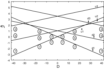
Figure 1: Deformed single-particle energies, $e_{i}=e_{i}^{0}-\chi d_{i}\sigma_{i}D$, plotted as functions of the deformation parameter $D$ for a set of parameters: $e_{j_{1}}^{0}=0.0,~{}e_{j_{2}}^{0}=1.0,~{}e_{j_{3}}^{0}=3.5$, $\Omega_{j_{1}}=14,~{}\Omega_{j_{2}}=10,~{}\Omega_{j_{3}}=4$, and $d_{j_{1}}=2,~{}d_{j_{2}}=d_{j_{3}}=1$. Numbers enclosed by circles indicate the numbers of pairs occupying individual levels in the lowest energy configuration for a given value of $D$ when pairing correlations are absent. Near the spherical point ($D=0$), the lowest shell is fully occupied by 14 pairs (28 nucleons). The level diagram is symmetric with respect to the sign-change of $D$ (prolate-oblate symmetry). The down(up)-sloping levels (with increasing $D$) are named “d1,d2, and d3 (u1,u2, and u3)”. In the prolate side ($D\geq 0$), the down-sloping level originating from the second shell (d2) crosses the up-sloping level (u1) at $D=8.3$. After this first crossing, the lowest-energy configuration involves 5 pairs occupying the second down-sloping level (d2) and 2 pairs remaining in the first up-sloping level (u1). At $D=29.2$, the down-sloping level originating from the third shell (d3) crosses the second up-sloping level (u2). In the lowest-energy configuration after this crossing, all the down-sloping levels are fully occupied while all the up-sloping levels are unoccupied. This configuration possesses the maximum value of the deformation parameter, $D_{\rm max}=42$. The same pattern of level crossings is valid also for the oblate side ($D\leq 0$). Note that this figure is drawn by regarding $D$ as a free parameter, although $D$ in Eq. (25) means an expectation value of the operator $\hat{D}$. In this sense this figure should be regarded as a kind of Nilsson diagram.

Figure 1 illustrates the single-particle energy diagram as a function of $D$. Details of the level crossings are explained in the caption to this figure. It is certainly possible to discuss the level crossing dynamics and simulate the shape coexistence phenomena by means of the multi-$O(4)$ model consisting of only two shells. However, consideration of the three shells is found to be more appropriate in order to make properties in the large deformation region more realistic. In realistic situations, a number of successive level crossings take place with increasing deformation.

5.3 Collective potentials

We present in Fig. 2 the collective potentials calculated for three values of the pairing strength $G$. For $G=0.14$, it exhibits a double well structure, while it looks like an anharmonic-oscillator potential for $G=0.2$. The case of $G=0.16$ shows a transitional character between these two situations. Note that the collective potentials are plotted here as functions of deformation $D$. The relation between $D$ and the collective coordinate $q$ will be explicitly shown later. The mechanism of appearance and disappearance of the double well structure is determined by competition between the pairing and “quadrupole” interactions: The pairing force favors an equal population of particles over all magnetic substates in each $j$-shell, whereas the “quadrupole” force favors an occupation of down-sloping levels creating level crossings and asymmetry in the magnetic substate population. In the three $j$-shell case under consideration, the energy of the degenerate local minima is lower than that of the spherical point for small values of $G$. With increasing pairing correlations, however, the energy of the spherical point decreases, so that the barrier hight decreases and eventually the barrier itself diminishes.

Figure 2: Collective potentials calculated with the ASCC method for $G=0.14$ (top), $G=0.16$ (middle), and $G=0.20$ (bottom) are plotted by solid lines as functions of deformation $D$. Other parameters used in the calculation are listed in the caption to Fig. 1. For comparison, collective potentials of the CHB method are indicated by dotted lines. Horizontal solid lines indicate eigen-energies of the quantized collective Hamiltonian.

In Fig. 2, quantum eigenstates obtained by solving the collective Shrödinger equations are indicated. We can clearly see a parity-doublet-like pattern associated with tunneling through the central barrier in the collective potential curve. Properties of these excitation spectra will be discussed in the succeeding subsection. In this figure, we also show the potential energy functions calculated by means of the conventional constrained HB (CHB) procedure:

$$V_{\rm CHB}(D)=\langle\phi_{0}^{\rm CHB}(D)|\hat{H}|\phi_{0}^{\rm CHB}(D)\rangle=2\sum_{i}e^{0}_{i}v_{i}^{2}-\frac{\Delta^{2}}{G}-\frac{1}{2}\chi D^{2},$$ (63)

where the state vectors $|\phi_{0}^{\rm CHB}(D)\rangle$ are determined by the constrained variational principle

$$\delta\langle\phi_{0}^{\rm CHB}(D)|{\hat{H}}-\lambda{\hat{N}}-\mu{\hat{D}}|\phi_{0}^{\rm CHB}(D)\rangle=0,$$ (64)

with $\mu$ denoting a Lagrange multiplier. As we see, the collective potentials obtained with the ASCC and CHB methods are practically indistinguishable. In principle, when both the collective path obtained in the ASCC method and that in the CHB method go through the same HB local minima, the collective potential energies at these points should coincide with each other. One may notice, however, very small differences between their values at the HB local minima with $D\neq 0$ for the cases of $G=0.14$ and 0.16. These discrepancies are due to violation of Eq. (7) which accumulates in the numerical calculation starting from $D=0$, and indicate the amount of error associated with the computational algorithms adopted here, as mentioned in subsection 6.1.

In Fig. 3, the pairing gaps $\Delta$ are shown as functions of deformation $D$. They monotonically decrease as $D$ increases, and vanish at the maximum deformation, which is $D_{\rm max}=42$ for the parameters adopted in these calculations. In Fig. 4, occupation probabilities $v_{i}^{2}$ are displayed. Note that all down-sloping (up-sloping) levels are fully occupied (unoccupied) at $D_{\rm max}$. Again, the results obtained with the ASCC and CHB methods are practically indistinguishable in these figures. Thus, in the present multi-$O(4)$ model, the static mean-field properties, like the potential energy curves and the pairing gaps, obtained with the ASCC method, are very similar to those obtained with the conventional CHB method. This is due to the simplicity of the multi-$O(4)$ model adopted here, and the collective subspace in general may differ from that of the CHB method  rf:27.

Figure 3: Pairing gaps $\Delta$ calculated with the ASCC method for $G=0.14$ (top), $G=0.16$ (middle), and $G=0.20$ (bottom) are plotted by solid lines as functions of deformation $D$. Other parameters used are the same as in Fig. 2. For comparison, $\Delta$ calculated with the CHB method and with the BCS approximation are also shown by dotted and dashed lines, respectively. The solid and dotted lines appear similar to each other. The equilibrium deformations are indicated by arrows.

Figure 4: Occupation probabilities $v_{i}^{2}$ calculated with the ASCC method for $G=0.14$ (top), $G=0.16$ (middle), and $G=0.20$ (bottom) are plotted by solid lines as functions of the deformation $D$. Other parameters used are the same as in Fig. 2. For comparison, $v_{i}^{2}$ calculated with the CHB method and with the BCS approximation are also shown by dotted and dashed lines, respectively. The solid and dotted lines appear similar to each other. Note that, at the large deformation limit $D_{\rm max}$, all down-sloping (up-sloping) levels are fully occupied (unoccupied) in the cases of the ASCC and CHB methods, whereas it is not the case in the BCS approximation.

In Figs. 3 and 4, we have also shown the BCS pairing gaps and occupation probabilities calculated in the BCS approximation. In this approximation, single particle energies given by $e_{i}=e_{i}^{0}-\chi d_{i}\sigma_{i}D$ are used to solve the BCS equations, where the deformation $D$ is treated as an ad hoc parameter, neglecting the HB selfconsistency (25) in accord with phenomenological singe-particle potential models. The pairing gap $\Delta$ in the BCS approximation differs from those in the CHB and ASCC methods. Note that the BCS gaps do not vanish in the limit $D_{\rm max}$ in contrast to the HB selfconsistent pairing gaps. In the following we shall focus our attention on dynamical properties of tunneling motions between the oblate and prolate minima.

5.4 Excitation spectra and collective mass

Figure 5 shows the excitation spectra and transition matrix elements for the ASCC method and for the exact diagonalization in a basis set, Eq. (20). Wave functions of the low-lying states are displayed in Figs. 6 and 7. The collectivity of these states are apparent from the enhancement of the transition matrix elements in comparison with the single-particle ones $d_{j}($=1 or 2). We see that the ASCC method well reproduces the major characteristics of the exact spectra and transition properties. In view of the huge degrees of freedom involved in the model under consideration (the dimension of this shell model space is 1894), it is remarkable that the low-lying states can be described very well in terms of only the single collective coordinate $q$. In particular, we note that the emergence of the “parity splitting” pattern for weaker strength $G$ of the pairing interaction is well reproduced in the calculation. This implies that the ASCC method succeeds in describing the large amplitude tunneling motions through the barrier between the oblate and prolate local minima.

As is well known, the collective mass parameter represents inertia against change of the mean field. It is determined locally and changes as $D$ varies. Since we have set the scale of the collective coordinate $q$ such that the collective mass parameter $M(q)=B^{-1}(q)$ with respect to $q$ is unity, the collective kinetic energy can be written either by $q$ or $D$ as

$$\frac{1}{2}\dot{q}^{2}=\frac{1}{2}(\frac{dq}{dD}\dot{D})^{2}\equiv\frac{1}{2}M(D)\dot{D}^{2}.$$ (65)

Thus, we obtain the explicit expression for $M(D)$:

$$M(D)\equiv(\frac{dq}{dD})^{2}=(\frac{d}{dq}\sum_{i}2d_{i}\sigma_{i}v_{i}^{2}(q))^{-2}=(4\sum_{i}d_{i}\sigma_{i}u_{i}v_{i}P_{i}(q))^{-2}.$$ (66)

The collective mass $M(D)$ evaluated in this way is shown in Fig. 8 as a function of $D$. One immediately notice that the ASCC mass $M(D)$ diverges in the limit $D\to D_{\rm max}$. The reason is clearly understood by examining the relationship between $D$ and the collective coordinate $q$. It is shown in Fig. 9. We see that the value of $D$ saturates as it approach its limiting value $D_{\rm max}$. Thus, the derivative $dq/dD$, which corresponds to the collective mass $M(D)$ according to Eq. (66), diverges. Needless to say, this divergence is caused by the existence of the maximum value of $D$ which is an artifact of the model: If we increase the number of shells explicitly taken into account, this limit is removed by successive level crosings with increasing $D$.

Figure 5: Comparison of excitation spectra calculated with the ASCC method and and with the exact diagonalization for $G=0.14$ (top), $G=0.16$ (middle), and $G=0.20$ (bottom). For reference sake, excitation energies of the lowest RPA modes in the HFB local minima are also indicated. Other parameters used are the same as in Fig. 2. Numbers adjacent to vertical lines indicate transition matrix elements for the “quadrupole” operator ${\hat{D}}$. In the top panel, transition matrix elements between “parity doublets” are indicated with arrows.

Figure 6: Collective wave functions $\psi(D)$ for the ground and first excited states in Fig. 5, obtained with the ASCC method for $G=0.14$ (top), $G=0.16$ (middle), and $G=0.20$ (bottom). The equilibrium deformations are indicated by arrows. The $\psi(D)$ are defined by $\psi(D)=\psi(q)|\frac{\partial q}{\partial D}|^{\frac{1}{2}}$, where $\psi(q)$ are wave functions for the collective coordinate $q$. Thus, they are normalized as $\int|\psi(q)|^{2}dq=\int|\psi(q)|^{2}|\frac{\partial q}{\partial D}|dD=\int|\psi(D)|^{2}dD=1$.

Figure 7: The same as Fig. 6 but for the second and third excited states. For $G=0.2$, only the wave function for the second excited state is drawn.

Figure 8: Collective mass $M(D)$ calculated with the ASCC method for $G=0.14$ (top), $G=0.16$ (middle), and $G=0.20$ (bottom) are plotted by solid lines as functions of deformation $D$. Other parameters used are the same as in Fig. 2. For comparison, the cranking mass are indicated by dotted lines. The equilibrium deformations are indicated by arrows.

Figure 9: Relations between the deformation $D$ and the collective coordinate $q$ in the ASCC method. The solid, dashed and dotted lines show the results of calculation for $G=0.14,0.16$, and 0.20, respectively.

It is interesting to compare the ASCC mass $M(D)$ with the cranking mass $M_{\rm cr}(D)$[1],

$$M_{\rm cr}(D) = 2\sum_{n}\frac{|\langle\phi_{n}^{\rm BCS}(D)|\frac{\partial}{\partial D}|\phi_{0}^{\rm BCS}(D)\rangle|^{2}}{E_{n}(D)-E_{0}(D)}$$ (67)

$$= 2\sum_{i}\frac{|2u_{i}v_{i}(\chi d_{i}\sigma_{i}+\frac{\partial\lambda}{\partial D})+(u^{2}_{i}-v^{2}_{i})\frac{\partial\Delta}{\partial D}|^{2}}{(2E_{i})^{3}}$$

where $\phi_{0}^{\rm BCS}(D)$ and $\phi_{n}^{\rm BCS}(D)$ represent the ground and excited states, and $E_{0}(D)$ and $E_{n}(D)$ the energies of them obtained in the BCS approximation. Namely, the coefficients of the Bogoliubov transformations, $u_{i},v_{i}$, the pairing gap $\Delta$, the chemical potential $\lambda$, and the quasiparticle energies $E_{i}$ are evaluated with use of single-particle energies defined by $e_{i}=e_{i}^{0}-\chi d_{i}\sigma_{i}D$. It is important to note that the deformation $D$ is treated in the BCS approximation as an ad hoc potential parameter disregarding the selfconsistency condition (25). Figure 8 shows that the cranking mass $M_{\rm cr}(D)$ is significantly different from the ASCC mass $M(D)$ in the whole interval of the deformation $D$, including the spherical point $D=0$ and the deformed equilibrium points. The difference between the ASCC mass and the cranking mass can be understood in terms of the HB selfconsistency.

At the spherical point ($D=0$), we can make the comparison between the ASCC mass and the cranking mass in an explicit way. There, all terms linear with respect to $\sigma_{i}$ in the local harmonic equations vanish after summing over all levels $i$ so that the pairing and “quadrupole” normal modes are exactly decoupled. Thus, we get a simple expression of the ASCC mass

$$M(D=0)=2\chi^{2}\sum_{i}\frac{2E_{i}(2d_{i}\sigma_{i}u_{i}v_{i})^{2}}{((2E_{i})^{2}-\omega^{2})^{2}}=4\chi^{2}\Delta^{2}\sum_{i}\frac{d_{i}^{2}}{E_{i}((2E_{i})^{2}-\omega^{2})^{2}}.$$ (68)

On the other hand, the expression of the cranking mass $M_{\rm cr}(D)$ reduces to

$$M_{\rm cr}(D=0)=\frac{1}{4}\chi^{2}\Delta^{2}\sum_{i}\frac{d_{i}^{2}}{E_{i}^{5}},$$ (69)

since the derivatives, $\partial\Delta/\partial D$ and $\partial\lambda/\partial D$ vanish at $D=0$. We see that the above expression for $M_{\rm cr}(D=0)$ can be related to $M(D=0)$ if we set $\omega=0$ in Eq. (68). In reality, the frequency $\omega$ is imaginary and $\omega^{2}$ is negative when the barrier exists ($G=0.14$ and 0.16). Accordingly, $M(D=0)\leq M_{\rm cr}(D=0)$ in these cases. On the other hand, $\omega$ is real and $\omega^{2}$ is positive when the spherical point is stable ($G=0.20$), so that $M(D=0)\geq M_{\rm cr}(D=0)$ in this case. In this way, the difference between the ASCC mass and the cranking mass in the barrier region (near $D\approx 0$) noticeable in Fig. 8 can be understood in terms of the finite frequency effect of the local harmonic mode, which is connected with the curvature of the collective potential by Eq. (58). This finite frequency effect decreases (increases) the collective mass when the barrier emerges (diminishes). We would like to emphasize that the finite frequency effect in the local harmonic equations represents selfconsistent dynamics of the time-dependent mean-field.

We note that, in contrast to the ASCC mass $M(D)$, the cranking mass $M_{\rm cr}(D)$ does not diverge at $D_{\rm max}$. This is because, as already emphasized above, the deformation $D$ is treated as an ad hoc parameter in the single-particle potential, so that the existence of the limit $D_{\rm max}$ in the selfconsistent deformation defined by Eq. (25) is disregarded there. In the multi-$O(4)$ model under consideration, the selfconsistency between the deformation parameter specifying the single-particle potential and the density deformation evaluated in terms of the wave function becomes extremely important near $D_{\rm max}$.

The comparison between the ASCC and cranking masses in Fig. 8 thus indicates the importance of the HB selfconsistency in evaluating the collective mass, although it is somewhat exaggerated because of an artificial aspect of the present parameter setting of the multi-$O(4)$ model.

There are various microscopic approaches to derive the collective mass (also called inertial functions)[1, 2, 31]. Certainly, it is important and interesting to make a detailed comparison of different approaches for the collective mass in the multi-$O(4)$ model, and clarify the role of the HB selfconsistency in more detail. Such a more systematic and comparative study is beyond the scope of this paper, but will be pursued in a separate paper.

6 Conclusions

The ASCC method was applied to the exactly solvable multi-$O(4)$ model which simulates nuclear shape coexistence phenomena. The collective mass and dynamics of large amplitude collective motions in this model system were analysed, and it was shown that the method can well describe the tunneling motions through the barrier between the prolate and oblate local minima in the collective potential. The result of numerical analysis strongly encourages applications of this approach to realistic cases. We plan to investigate the oblate-prolate shape coexistence phenomena in ⁶⁸Se with use of the P+Q interactions.

References

- [1] P. Ring and P. Schuck, The Nuclear Many-Body Problem (Springer-Verlag, 1980).
- [2] J.-P. Blaizot and G. Ripka, Quantum Theory of Finite Systems (The MIT press, 1986).
- [3] D.J. Rowe and R. Bassermann, \JLCanad.J.Phys.,54,1976,1941.
- [4] K. Goeke, \NPA265,1976,301.
- [5] F. Villars, \NPA285,1977,269.
- [6] T. Marumori, \PTP57,1977,112.
- [7] M. Baranger and M. Veneroni, \ANN114,1978,123.
- [8] K. Goeke and P.-G. Reinhard, \ANN112,1978,328.
- [9] T. Marumori, T. Maskawa, F. Sakata, and A.Kuriyama, \PTP64,1980,1294.
- [10] M.J. Giannoni and P. Quentin, \PRC21,1980,2060.
- [11] J. Dobaczewski and J. Skalski, \NPA369,1981,123.
- [12] K. Goeke, P.-G. Reinhard, and D.J. Rowe, \NPA359,1981,408.
- [13] A.K. Mukherjee and M.K. Pal, \PLB100,1981, 457. \NPA373,1982,289.
- [14] D. J. Rowe, \NPA391,1982,307.
- [15] C. Fiolhais and R.M. Dreizler, \NPA393,1983,205.
- [16] K. Goeke, F. Grümmer, and P.-G. Reinhard, \ANN150,1983,504.
- [17] A. Kuriyama and M. Yamamura, \PTP70,1983,1675.;\JL,71 ,1984, 122.
- [18] M. Yamamura, A. Kuriyama, and S. Iida, \PTP71,1984,109.
- [19] M. Matsuo and K. Matsuyanagi, \PTP74,1985,288.
- [20] M. Matsuo, \PTP76,1986,372.
- [21] Y.R. Shimizu and K. Takada, \PTP77,1987,1192.
- [22] M. Yamamura and A. Kuriyama, \PTPS93,1987.
- [23] N.R. Walet, G. Do Dang, and A. Klein, \PRC43,1991,2254.
- [24] A. Klein, N.R. Walet, and G. Do Dang, \ANN208,1991,90.
- [25] K. Kaneko, \PRC49,1994,3014.
- [26] T. Nakatsukasa and N.R. Walet, \PRC57,1998,1192.
- [27] T. Nakatsukasa and N.R. Walet, \PRC58,1998,3397.
- [28] J. Libert, M. Girod and J.-P. Delaroche, \PRC60,1999,054301.
- [29] E.Kh. Yuldashbaeva, J. Libert, P. Quentin and M. Girod, \PLB461,1999,1.
- [30] T. Nakatsukasa, N.R. Walet, and G. Do Dang, \PRC61,2000,014302.
- [31] G. Do Dang, A. Klein, and N.R. Walet, \PRP335,2000,93.
- [32] J.L. Wood, K. Heyde, W. Nazarewicz, M. Huyse, and P. van Duppen, \PRP215,1992,101.
- [33] W. Nazarewicz, \PLB305,1993,195.
- [34] W. Nazarewicz, \NPA557,1993,489c.
- [35] N. Tajima, H. Flocard, P. Bonche, J. Dobaczewski, and P.-H. Heenen, \NPA551,1993,409.
- [36] P. Bonche, E. Chabanat, B.Q. Chen, J. Dobaczewski, H. Flocard, B. Gall, P.H. Heenen, J. Meyer, N. Tajima, and M.S. Weiss, \NPA574,1994,185c.
- [37] P.-G. Reinhard, D.J. Dean, W. Nazarewicz, J. Dobaczewski, J.A. Maruhn, and M.R. Strayer, \PRC60,1999,014316.
- [38] A.N. Andreyev et al., \JLNature,405,2000,430.; \NPA682,2001,482c.
- [39] S.M. Fischer et al., \PRL84,2000,4064.
- [40] R.R. Rodríguez-Guzmán, J.L. Egido, and L.M. Robledo, \PRC62,2000,054319.;\JLC,65,2002,024304.
- [41] R.R. Chasman, J.L. Egido, L.M. Robledo, \PLB513,2001,325.
- [42] T. Nikšić, D. Vretenar, P. Ring, and G.A. Lalazissis, \PRC65,2002,054320.
- [43] A. Petrovici, K.W. Schmid, and A. Faessler, \NPA710,2002,246.
- [44] T. Duguet, M. Bender, P. Bonche, and P.-H. Heenen, preprint nucl-th/0212016.
- [45] R. Fossion, K. Heyde, G. Thiamova, and P. Van Isacker, preprint nucl-th/0301029.
- [46] M. Matsuo, \PTP72,1984,666.
- [47] M. Matsuo and K. Matsuyanagi, \PTP74,1985,1227.; \JL,76,1986,93.; \JL,78,1987,591.
- [48] M. Matsuo, Y. R. Shimizu, and K. Matsuyanagi, Proceedings of The Niels Bohr Centennial Conf. on Nuclear Structure, ed. R. Broglia, G. Hagemann and B. Herskind (North-Holland, 1985), p. 161.
- [49] K. Takada, K. Yamada, and H. Tsukuma, \NPA496,1989,224.
- [50] K. Yamada, K. Takada, and H. Tsukuma, \NPA496,1989,239.
- [51] K. Yamada and K. Takada, \NPA503,1989,53.
- [52] H. Aiba, \PTP84,1990,908.
- [53] K. Yamada, \PTP85,1991,805;\JL89,1993,995.
- [54] J. Terasaki, T. Marumori, and F. Sakata, \PTP85,1991,1235.
- [55] J. Terasaki, \PTP88,1992,529;\JL92,1994,535.
- [56] M. Matsuo, in New Trends in Nuclear Collective Dynamics, (Springer-Verlag, 1992), eds. Y. Abe, H. Horiuchi and K. Matsuyanagi, p.219.
- [57] Y.R. Shimizu and K. Matsuyanagi, \PTPS141,2001,285.
- [58] M. Matsuo, T. Nakatsukasa, and K. Matsuyanagi, \PTP103,2000,959.
- [59] M. Baranger and K. Kumar, \JLNucl. Phys, 62 ,1965, 113.; \JLA ,100,1967, 490.; \JLA, 110,1968, 529.;\JLA, 122, 1968, 241.;\JLA, 122 ,1968, 273.
- [60] D. R. Bes and R. A. Sorensen, Advances in Nuclear Physics (Prenum Press, 1969), vol. 2, p. 129.
- [61] K. Matsuyanagi, \PTP67,1982,1141.; Proceedings of the Nuclear Physics Workshop, Trieste, 5-30 Oct. 1981. ed. C.H. Dasso, R.A. Broglia and A. Winther (North-Holland, 1982), p.29.
- [62] Y. Mizobuchi, \PTP65,1981,1450.
- [63] T. Suzuki and Y. Mizobuchi, \PTP79,1988,480.
- [64] T. Fukui, M. Matsuo and K. Matsuyanagi, \PTP85,1991,281.
- [65] P.O. Arve and G.F. Bertsch, \PLB215,1988,1.