Unifying aspects of light- and heavy-systems

Abstract

Dyson-Schwinger equations furnish a Poincaré covariant framework within which to study hadrons. A particular feature is the existence of a nonperturbative, symmetry preserving truncation that enables the proof of exact results. Key to the DSE’s efficacious application is their expression of the materially important momentum-dependent dressing of parton propagators at infrared length-scales, which is responsible for the magnitude of constituent-quark masses and the length-scale characterising confinement in bound states. A unified quantitative description of light- and heavy-quark systems is achieved by capitalising on these features.

1 Introduction

This contribution provides an overview of one particular means by which a quantitative and intuitive understanding of strong interaction phenomena can be attained. The broad framework is that of continuum strong QCD, by which I mean the continuum nonperturbative methods and models that can address these phenomena, especially those where a direct connection with QCD can be established, in one true limit or another. Naturally, everyone has a favourite tool and, in this connection, the Dyson-Schwinger equations (DSEs) are mine cdragw . The framework is appropriate here because the last decade has seen a renaissance in its phenomenological application, with studies of phenomena as apparently unconnected as low-energy $\pi\pi$ scattering, $B\to D^{\ast}$ decays and the equation of state for a quark gluon plasma bastirev ; reinhardrev ; pieterrev . Indeed, the DSEs promise a single structure applicable to the gamut of strong interaction observables.

Dyson-Schwinger equations provide a nonperturbative means of analysing a quantum field theory. Derived from a theory’s Euclidean space generating functional, they are an enumerable infinity of coupled integral equations whose solutions are the $n$-point Schwinger functions (Euclidean Green functions), which are the same matrix elements estimated in numerical simulations of lattice-QCD. In theories with elementary fermions, the simplest of the DSEs is the gap equation, which is basic to studying dynamical symmetry breaking in systems as disparate as ferromagnets, superconductors and QCD. The gap equation is a good example because it is familiar and has all the properties that characterise each DSE. Its solution is a $2$-point function (the fermion propagator) but its kernel involves higher $n$-point functions; e.g., in a gauge theory, the kernel is constructed from the gauge-boson $2$-point function and fermion–gauge-boson vertex, a $3$-point function. In addition, while a weak-coupling expansion yields all the diagrams of perturbation theory, a self-consistent solution of the gap equation exhibits nonperturbative effects unobtainable at any finite order in perturbation theory; e.g, dynamical chiral symmetry breaking (DCSB).

The coupling between equations; namely, the fact that the equation for a given $m$-point function always involves at least one $n>m$-point function, necessitates a truncation of the tower of DSEs in order to define a tractable problem. It is unsurprising that the best known truncation scheme is just the weak coupling expansion which reproduces every diagram in perturbation theory. This scheme is systematic and valuable in the analysis of large momentum transfer processes because QCD is asymptotically free. However, it precludes the study of nonperturbative effects, and hence something else is needed for the investigation of strongly interacting systems and bound state phenomena.

In spite of the need for a truncation, gap equations have long been used effectively in obtaining nonperturbative information about many-body systems as, e.g., in the Nambu-Gorkov formalism for superconductivity. The positive outcomes have been achieved through the simple expedient of employing the most rudimentary truncation, e.g., Hartree or Hartree-Fock, and comparing the results with observations. Of course, agreement under these circumstances is not an unambiguous indication that the contributions omitted are small nor that the model expressed in the truncation is sound. However, it does justify further study, and an accumulation of good results is grounds for a concerted attempt to substantiate a reinterpretation of the truncation as the first term in a systematic and reliable approximation.

The modern application of DSEs, notably, comparisons with and predictions of experimental data, can properly be said to rest on model assumptions. However, those assumptions can be tested within the framework and also via comparison with lattice-QCD simulations, and the predictions are excellent. Furthermore, progress in understanding the intimate connection between symmetries and truncation schemes has enabled exact results to be proved. Herein I will briefly explain recent phenomenological applications and the foundation of their success, and focus especially on the links the approach provides between light- and heavy-quark phenomena. It will become apparent that the momentum-dependent dressing of the propagators of QCD’s elementary excitations is a fundamental and observable feature of strong QCD.

The article is organised as follows: Sec. 2 [p. 2] – a review of DSE quiddities, especially in connection with the development of a nonperturbative, systematic and symmetry preserving truncation scheme, and the model-independent results whose proof its existence enables; Sec. 3 [p. 3] – an illustration of the efficacious application of DSE methods to light-meson systems and the connections that may be made with the results of lattice-QCD simulations; Sec. 4 [p. 4] – the natural extension of these methods to heavy-quark systems, with an explanation of the origin and derivation of heavy-quark symmetry limits and their confrontation with the real-world of finite quark masses; and Sec. 5 [p. 5] – an epilogue.

2 Dyson-Schwinger Equations

2.1 Gap Equation

The simplest DSE is the gap equation, which describes how the propagation of a fermion is modified by its interactions with the medium being traversed. In QCD that equation assumes the form:

$$S^{-1}(p)\!=\!Z_{2}(\zeta,\Lambda)\,i\,\gamma\cdot p+Z_{4}(\zeta,\Lambda)\,m(\zeta)+\Sigma^{\prime}(p,\Lambda),$$ (1)

wherein the dressed-quark self-energy is

$$\Sigma^{\prime}(p,\Lambda)=Z_{1}(\zeta,\Lambda)\!\int^{\Lambda}_{q}\!\!\!g^{2}D_{\mu\nu}(p-q)\,\frac{\lambda^{i}}{2}\gamma_{\mu}\,S(q)\,\Gamma^{i}_{\nu}(q,p).$$ (2)

Equations (1), (2) constitute the renormalised DSE for the dressed-quark propagator. In Eq. (2), $D_{\mu\nu}(k)$ is the renormalised dressed-gluon propagator, $\Gamma^{a}_{\nu}(q;p)$ is the renormalised dressed-quark-gluon vertex and $\int^{\Lambda}_{q}:=\int^{\Lambda}d^{4}q/(2\pi)^{4}$ represents a translationally-invariant regularisation of the integral, with $\Lambda$ the regularisation mass-scale.  In addition, $Z_{1}(\zeta,\Lambda)$, $Z_{2}(\zeta,\Lambda)$ and $Z_{4}(\zeta,\Lambda)$ are, respectively, Lagrangian renormalisation constants for the quark-gluon vertex, quark wave function and quark mass-term, which depend on the renormalisation point, $\zeta$, and the regularisation mass-scale, as does the gauge-independent mass renormalisation constant,

$$Z_{m}(\zeta^{2},\Lambda^{2})=Z_{4}(\zeta^{2},\Lambda^{2})\,Z_{2}^{-1}(\zeta^{2},\Lambda^{2})\,,$$ (3)

whereby the renormalised running-mass is related to the bare mass:

$$m(\zeta)=Z_{m}^{-1}(\zeta^{2},\Lambda^{2})\,m_{\rm bm}(\Lambda)\,.$$ (4)

When $\zeta$ is very large the running-mass can be evaluated in perturbation theory, which gives

$$m(\zeta)=\frac{\hat{m}}{(\ln\zeta/\Lambda_{\rm QCD})^{\gamma_{m}}\!\!\!\!\!\!\!}\;\;\;\;\;,\;\gamma_{m}=12/(33-2N_{f})\,.$$ (5)

Here $N_{f}$ is the number of current-quark flavours that contribute actively to the running coupling, and $\Lambda_{\rm QCD}$ and $\hat{m}$ are renormalisation group invariants.

The solution of Eq. (1) is the dressed-quark propagator and takes the form

$$S^{-1}(p)=i\gamma\cdot p\,A(p^{2},\zeta^{2})+B(p^{2},\zeta^{2})\\ \equiv\frac{1}{Z(p^{2},\zeta^{2})}\left[i\gamma\cdot p+M(p^{2})\right].$$ (6)

It is obtained by solving the gap equation subject to the renormalisation condition that at some large spacelike $\zeta^{2}$

$$\left.S^{-1}(p)\right|_{p^{2}=\zeta^{2}}=i\gamma\cdot p+m(\zeta)\,.$$ (7)

The observations made in in the Introduction are now manifest. The gap equation is a nonlinear integral equation for $S(p)$ and can therefore yield much-needed nonperturbative information. However, the kernel involves the two-point function $D_{\mu\nu}(k)$ and the three-point function $\Gamma^{a}_{\nu}(q;p)$. The equation is consequently coupled to the DSEs these functions satisfy and hence a manageable problem is obtained only once a truncation scheme is specified.

2.2 Nonperturbative Truncation

To understand why Eq. (1) is called a gap equation, consider the chiral limit, which is readily defined mrt98 because QCD exhibits asymptotic freedom and implemented in the gap equation by employing mr97

$$Z_{2}(\zeta^{2},\Lambda^{2})\,m_{\rm bm}(\Lambda)\equiv 0\,,\;\;\Lambda\gg\zeta\,.$$ (8)

It is noteworthy that for finite $\zeta$ and $\Lambda\to\infty$, the left hand side (l.h.s.) of Eq. (8) is identically zero, by definition, because the mass term in QCD’s Lagrangian density is renormalisation-point-independent. The condition specified in Eq. (8), on the other hand, effects the result that at the (perturbative) renormalisation point there is no mass-scale associated with explicit chiral symmetry breaking, which is the essence of the chiral limit. An equivalent statement is that one obtains the chiral limit when the renormalisation-point-invariant current-quark mass vanishes; namely, $\hat{m}=0$ in Eq. (5). In this case the theory is chirally symmetric, and a perturbative evaluation of the dressed-quark propagator from Eq. (1) gives

$$B_{\rm pert}^{0}(p^{2}):=\lim_{m\to 0}B_{\rm pert}(p^{2})=\lim_{m\to 0}m\left(1-\frac{\alpha}{\pi}\ln\left[\frac{p^{2}}{m^{2}}\right]+\ldots\right)\equiv 0\,;$$ (9)

viz., the perturbative mass function is identically zero in the chiral limit. It follows that there is no gap between the top level in the quark’s filled negative-energy Dirac sea and the lowest positive energy level.

However, suppose one has at hand a truncation scheme other than perturbation theory and that subject to this scheme Eq. (1) possessed a chiral limit solution $B^{0}(p^{2})\not\equiv 0$. Then interactions between the quark and the virtual quanta populating the ground state would have nonperturbatively generated a mass gap. The appearance of such a gap breaks the theory’s chiral symmetry. This shows that the gap equation can be an important tool for studying DCSB, and it has long been used to explore this phenomenon in both QED and QCD cdragw .

The gap equation’s kernel is formed from a product of the dressed-gluon propagator and dressed-quark-gluon vertex but in proposing and developing a truncation scheme it is insufficient to focus only on this kernel mr97 ; raya . The gap equation can only be a useful tool for studying DCSB if the truncation itself does not destroy chiral symmetry.

Chiral symmetry is expressed via the axial-vector Ward-Takahashi identity:

$$P_{\mu}\,\Gamma_{5\mu}(k;P)=S^{-1}(k_{+})\,i\gamma_{5}+i\gamma_{5}\,S^{-1}(k_{-})\,,\;k_{\pm}=k\pm P/2,$$ (10)

wherein $\Gamma_{5\mu}(k;P)$ is the dressed axial-vector vertex. This three-point function satisfies an inhomogeneous Bethe-Salpeter equation (BSE):

$$\left[\Gamma_{5\mu}(k;P)\right]_{tu}=Z_{2}\left[\gamma_{5}\gamma_{\mu}\right]_{tu}+\int^{\Lambda}_{q}[S(q_{+})\Gamma_{5\mu}(q;P)S(q_{-})]_{sr}K_{tu}^{rs}(q,k;P)\,,$$ (11)

in which $K(q,k;P)$ is the fully-amputated quark-antiquark scattering kernel, and the colour-, Dirac- and flavour-matrix structure of the elements in the equation is denoted by the indices $r,s,t,u$. The Ward-Takahashi identity, Eq. (10), entails that an intimate relation exists between the kernel in the gap equation and that in the BSE. (This is another example of the coupling between DSEs.) Therefore an understanding of chiral symmetry and its dynamical breaking can only be obtained with a nonperturbative truncation scheme that preserves this relation, and hence guarantees Eq. (10) without a fine-tuning of model-dependent parameters.

Rainbow-ladder truncation.

At least one such scheme exists truncscheme . Its leading-order term is the so-called renormalisation-group-improved rainbow-ladder truncation, whose analogue in the many body problem is an Hartree-Fock truncation of the one-body (Dyson) equation combined with a consistent ladder-truncation of the related two-body (Bethe-Salpeter) equation. To understand the origin of this leading-order term, observe that the dressed-ladder truncation of the quark-antiquark scattering kernel is expressed in Eq. (11) via

$$[L(q,k;P)]_{tu}^{t^{\prime}u^{\prime}}\,[\Gamma_{5\mu}(q;P)]_{u^{\prime}t^{\prime}}:=[S(q_{+})\Gamma_{5\mu}(q;P)S(q_{-})]_{sr}\,K_{tu}^{rs}(q,k;P)$$ (12)

$$= -g^{2}(\zeta^{2})\,D_{\rho\sigma}(k-q)\,$$

$$\times\left[\rule{0.0pt}{8.39996pt}\Gamma^{a}_{\rho}(k_{+},q_{+})\,S(q_{+})\right]_{tt^{\prime}}\left[\rule{0.0pt}{8.39996pt}S(q_{-})\,\Gamma^{a}_{\sigma}(q_{-},k_{-})\right]_{u^{\prime}u}\,[\Gamma_{5\mu}(q;P)]_{t^{\prime}u^{\prime}}$$

wherein I have only made explicit the renormalisation point dependence of the coupling. One can exploit multiplicative renormalisability and asymptotic freedom to demonstrate that on the kinematic domain for which $Q^{2}:=(k-q)^{2}\sim k^{2}\sim q^{2}$ is large and spacelike

$$[L(q,k;P)]_{tu}^{t^{\prime}u^{\prime}}=-4\pi\alpha(Q^{2})\,D_{\rho\sigma}^{\rm free}(Q)\,\left[\rule{0.0pt}{8.39996pt}\frac{\lambda^{a}}{2}\gamma_{\rho}\,S^{\rm free}(q_{+})\right]_{tt^{\prime}}\left[\rule{0.0pt}{8.39996pt}S^{\rm free}(q_{-})\,\frac{\lambda^{a}}{2}\gamma_{\sigma}\right]_{u^{\prime}u}\!,$$ (13)

where $\alpha(Q^{2})$ is the strong running coupling and, e.g., $S^{\rm free}$ is the free quark propagator. It follows that on this domain the r.h.s. of Eq. (13) describes the leading contribution to the complete quark-antiquark scattering kernel, $K_{tu}^{rs}(q,k;P)$, with all other contributions suppressed by at least one additional power of $1/Q^{2}$.

The renormalisation-group-improved ladder-truncation supposes that

$$K_{tu}^{rs}(q,k;P)=-4\pi\,\alpha(Q^{2})\,D_{\rho\sigma}^{\rm free}(Q)\,\left[\rule{0.0pt}{8.39996pt}\frac{\lambda^{a}}{2}\gamma_{\rho}\right]_{ts}\left[\rule{0.0pt}{8.39996pt}\frac{\lambda^{a}}{2}\gamma_{\sigma}\right]_{ru}$$ (14)

is also a good approximation on the infrared domain and is thus an assumption about the long-range ($Q^{2}\mathrel{\hbox to0.0pt{\lower 4.0pt\hbox{\hskip 0.0pt$\sim$}\hss}\raise 1.0pt\hbox{$<$}}1\,$ GeV²) behaviour of the interaction. Combining Eq. (14) with the requirement that Eq. (10) be automatically satisfied leads to the renormalisation-group-improved rainbow-truncation of the gap equation:

$$S^{-1}(p)=Z_{2}\,(i\gamma\cdot p+m_{\rm bm})+\int^{\Lambda}_{q}\!4\pi\,\alpha(Q^{2})\,D_{\mu\nu}^{\rm free}(p-q)\frac{\lambda^{a}}{2}\gamma_{\mu}\,S(q)\,\frac{\lambda^{a}}{2}\gamma_{\nu}\,.$$ (15)

This rainbow-ladder truncation provides the foundation for an explanation of a wide range of hadronic phenomena pieterrev .

2.3 Systematic Procedure

The truncation scheme of Ref. truncscheme is a dressed-loop expansion of the dressed-quark-gluon vertices that appear in the half-amputated dressed-quark-antiquark scattering matrix: $S^{2}K$, a renormalisation-group invariant detmold . All $n$-point functions involved thereafter in connecting two particular quark-gluon vertices are fully dressed. The effect of this truncation in the gap equation, Eq. (1), is realised through the following representation of the dressed-quark-gluon vertex, $i\Gamma_{\mu}^{a}=\frac{i}{2}\lambda^{a}\,\Gamma_{\mu}=l^{a}\Gamma_{\mu}$:

$$Z_{1}\Gamma_{\mu}(k,p)=\gamma_{\mu}+\frac{1}{2N_{c}}\int_{\ell}^{\Lambda}\!g^{2}D_{\rho\sigma}(p-\ell)\gamma_{\rho}S(\ell+k-p)\gamma_{\mu}S(\ell)\gamma_{\sigma}$$

$$+ \frac{N_{c}}{2}\int_{\ell}^{\Lambda}\!g^{2}\,D_{\sigma^{\prime}\sigma}(\ell)\,D_{\tau^{\prime}\tau}(\ell+k-p)\,\gamma_{\tau^{\prime}}\,S(p-\ell)\,\gamma_{\sigma^{\prime}}\,\Gamma^{3g}_{\sigma\tau\mu}(\ell,-k,k-p)+[\ldots]\,.$$

(16)

Here $\Gamma^{3g}$ is the dressed-three-gluon vertex and it is readily apparent that the lowest order contribution to each term written explicitly is O$(g^{2})$. The ellipsis represents terms whose leading contribution is O$(g^{4})$; viz., the crossed-box and two-rung dressed-gluon ladder diagrams, and also terms of higher leading-order.

This expansion of $S^{2}K$, with its implications for other $n$-point functions, yields an ordered truncation of the DSEs that guarantees, term-by-term, the preservation of vector and axial-vector Ward-Takahashi identities, a feature that has been exploited mrt98 ; marisAdelaide ; mishaSVY to establish exact results in QCD. It is readily seen that inserting Eq. (16) into Eq. (1) provides the rule by which the rainbow-ladder truncation can be systematically improved.

Planar vertex.

The effect of the complete vertex in Eq. (16) on the solutions of the gap equation is unknown. However, insights have been drawn from a study detmold of a more modest problem obtained by retaining only the sum of dressed-gluon ladders; i.e., the vertex depicted in Fig. 1. The elucidation is particularly transparent when one employs mn83

$${\cal D}_{\mu\nu}(k):=g^{2}\,D_{\mu\nu}(k)=\left(\delta_{\mu\nu}-\frac{k_{\mu}k_{\nu}}{k^{2}}\right)(2\pi)^{4}\,{\cal G}^{2}\,\delta^{4}(k)$$ (17)

for the dressed-gluon line, which defines an ultraviolet finite model so that the regularisation mass-scale can be removed to infinity and the renormalisation constants set equal to one.  This model has many positive features in common with the class of renormalisation-group-improved rainbow-ladder models and its particular momentum-dependence works to advantage in reducing integral equations to algebraic equations with similar qualitative features. There is naturally a drawback: the simple momentum dependence also leads to some model-dependent artefacts, but they are easily identified and hence not cause for concern.

The general form of the dressed-quark gluon vertex involves twelve distinct scalar form factors but using Eq. (17) only $\Gamma_{\mu}(p):=\Gamma_{\mu}(p,p)$ contributes to the gap equation, which considerably simplifies the analysis. The summation depicted in Fig. 1 is expressed via

$$\Gamma_{\mu}(p)=\gamma_{\mu}+\frac{1}{8}\,\gamma_{\rho}\,S(p)\,\Gamma_{\mu}(p)\,S(p)\,\gamma_{\rho}\,,$$ (18)

which supports a solution

$$\Gamma_{\mu}(p)=\alpha_{1}(p^{2})\,\gamma_{\mu}+\,\alpha_{2}(p^{2})\,\gamma\cdot p\,p_{\mu}-\,\alpha_{3}(p^{2})\,i\,p_{\mu}\,.$$ (19)

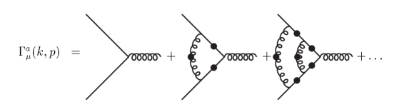
Figure 1: Integral equation for a planar dressed-quark-gluon vertex obtained by neglecting contributions associated with explicit gluon self-interactions. Solid circles indicate fully dressed propagators. The vertices are not dressed. (Adapted from Ref. detmold .)

One can re-express this vertex as

$$\Gamma_{\mu}(p)=\sum_{i=0}^{\infty}\,\Gamma_{\mu}^{i}(p)=\sum_{i=0}^{\infty}\,\left[\alpha^{i}_{1}(p^{2})\,\gamma_{\mu}+\,\alpha^{i}_{2}(p^{2})\,\gamma\cdot p\,p_{\mu}-\,\alpha^{i}_{3}(p^{2})\,i\,p_{\mu}\right],$$ (20)

where the superscript enumerates the order of the iterate: $\Gamma_{\mu}^{i=0}$ is the bare vertex,

$$\begin{array}[]{cc}\alpha_{1}^{0}=1\,,&\alpha_{2}^{0}=0=\alpha_{3}^{0}\,;\end{array}$$ (21)

$\Gamma_{\mu}^{i=1}$ is the result of inserting this into the r.h.s. of Eq (18) to obtain the one-rung dressed-gluon correction; $\Gamma_{\mu}^{i=2}$ is the result of inserting $\Gamma_{\mu}^{i=1}$, and is therefore the two-rung dressed-gluon correction; etc. A key observation detmold is that each iterate is related to its precursor via a simple recursion relation and, substituting Eq. (20), that recursion yields ($s=p^{2}$)

$$\mbox{\boldmath$\alpha$}^{i+1}(s):=\left(\begin{array}[]{l}\rule{0.0pt}{10.76385pt}\alpha_{1}^{i+1}(s)\\ \rule{0.0pt}{10.76385pt}\alpha_{2}^{i+1}(s)\\ \rule{0.0pt}{10.76385pt}\alpha_{3}^{i+1}(s)\end{array}\right)={\cal O}(s;A,B)\,\mbox{\boldmath$\alpha$}^{i}(s)\,,$$ (22)

$${\cal O}(s;A,B)=\frac{1}{4}\,\frac{1}{\Delta^{2}}\left(\begin{array}[]{ccc}\rule{0.0pt}{10.76385pt}-\Delta&0&0\\ \rule{0.0pt}{10.76385pt}2A^{2}&sA^{2}-B^{2}&2AB\\ \rule{0.0pt}{10.76385pt}4AB&4sAB&2(B^{2}-sA^{2})\end{array}\right),$$ (23)

$\Delta=sA^{2}(s)+B^{2}(s)$. It follows that

$$\mbox{\boldmath$\alpha$}=\left(\sum_{i=1}^{\infty}\,{\cal O}^{i}\right)\,\mbox{\boldmath$\alpha$}^{0}=\frac{1}{1-{\cal O}}\,\mbox{\boldmath$\alpha$}^{0}\,$$ (24)

and hence, using Eq. (21),

$$\alpha_{1} = \frac{4\,\Delta}{1+4\,\Delta}\,,$$

$$\alpha_{2} = \frac{-\,8\,A^{2}}{1+2\,(B^{2}-s\,A^{2})-8\,\Delta^{2}}\,\frac{1+2\,\Delta}{1+4\,\Delta}\,,$$ (25)

$$\alpha_{3} = \frac{-8\,AB}{1+2(B^{2}-s\,A^{2})-8\,\Delta^{2}}\,.$$

The recursion relation thus leads to a closed form for the gluon-ladder-dressed quark-gluon vertex in Fig. 1; viz., Eqs. (19), (25). Its momentum-dependence is determined by that of the dressed-quark propagator, which is obtained by solving the gap equation, itself constructed with this vertex. Using Eq. (17), that gap equation is

$$S^{-1}(p)=i\gamma\cdot p+m+\gamma_{\mu}\,S(p)\,\Gamma_{\mu}(p)\\$$ (26)

whereupon the substitution of Eq. (19) gives

$$A(s) = 1+\frac{1}{sA^{2}+B^{2}}\left[A\,(2\alpha_{1}-s\alpha_{2})-B\,\alpha_{3}\right]\,,$$ (27)

$$B(s) = m+\frac{1}{sA^{2}+B^{2}}\left[B\,(4\alpha_{1}+s\alpha_{2})-sA\,\alpha_{3}\right]\,.$$ (28)

Equations (27), (28), completed using Eqs. (25), form a closed algebraic system. It can easily be solved numerically, and that yields simultaneously the complete gluon-ladder-dressed vertex and the propagator for a quark fully dressed via gluons coupling through this nonperturbative vertex. Furthermore, it is apparent that in the chiral limit, $m=0$, a realisation of chiral symmetry in the Wigner-Weyl mode, which is expressed via the $B\equiv 0$ solution of the gap equation, is always admissible. This is the solution anticipated in Eq. (9).

Figure 2: $A(s)$, $M(s)$ obtained from Eqs. (25), (27), (28) with $m=0.023$ (solid line). All dimensioned quantities are expressed in units of ${\cal G}$ in Eq. (17). For comparison, the results obtained with the zeroth-order vertex (dotted line) and the one-loop vertex (dashed line) are also plotted. (Adapted from Ref. detmold .)

The chiral limit gap equation also admits a Nambu-Goldstone mode solution whose $p^{2}\simeq 0$ properties are unambiguously related to those of the $m\neq 0$ solution, a feature also evident in QCD mishaSVY . A complete solution of Eq. (26) is available numerically, and results for the dressed-quark propagator are depicted in Fig. 2. It is readily seen that the complete resummation of dressed-gluon ladders gives a dressed-quark propagator that is little different from that obtained with the one-loop-corrected vertex; and there is no material difference from the result obtained using the zeroth-order vertex. Similar observations apply to the vertex itself. The scale of these modest effects can be quantified by a comparison between the values of $M(s=0)=B(0)/A(0)$ calculated using vertices dressed at different orders:

$$\begin{array}[]{l||c|c|c|c}\sum_{i=0,N}\Gamma_{\mu}^{i}&N=0&N=1&N=2&N=\infty\\[6.45831pt] \hline\cr M(0)&\rule{0.0pt}{8.61108pt}1&1.105&1.115&1.117\end{array}$$ (29)

The rainbow truncation of the gap equation is accurate to within 12% and adding just one gluon ladder gives 1% accuracy. It is important to couple this with an understanding of how the vertex resummation affects the Bethe-Salpeter kernel.

Vertex-consistent Bethe-Salpeter kernel.

The renormalised homogeneous BSE for the quark-antiquark channel denoted by $M$ can be expressed

$$[\Gamma_{M}(k;P)]_{tu}=\int_{q}^{\Lambda}\![\chi_{M}(q;P)]_{sr}\,[K(k,q;P)]_{tu}^{rs}\,,$$ (30)

where: $\Gamma_{M}(k;P)$ is the meson’s Bethe-Salpeter amplitude, $k$ is the relative momentum of the quark-antiquark pair, $P$ is their total momentum; and

$$\chi_{M}(k;P)=S(k_{+})\,\Gamma_{M}(k;P)\,S(k_{-})\,.$$ (31)

Equation (30), depicted in Fig. 3, describes the residue at a pole in the solution of an inhomogeneous BSE; e.g., the lowest mass pole solution of Eq. (11) is identified with the pion.

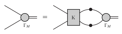
Figure 3: Homogeneous BSE, Eq. (30). Filled circles: dressed propagators or vertices; $K$ is the dressed-quark-antiquark scattering kernel. A systematic truncation of $S^{2}K$ is the key to preserving Ward-Takahashi identities truncscheme ; herman . (Adapted from Ref. detmold .)

I noted on p. 2.2 that the automatic preservation of Ward-Takahashi identities in those channels related to strong interaction observables requires a conspiracy between the dressed-quark-gluon vertex and the Bethe-Salpeter kernel truncscheme ; herman . A systematic procedure for building that kernel follows detmold from the observation herman that the gap equation can be expressed via

$$\frac{\delta\Gamma[S]}{\delta S}=0\,,$$ (32)

where $\Gamma[S]$ is a Cornwall-Jackiw-Tomboulis-like effective action haymaker . The Bethe-Salpeter kernel is then obtained via an additional functional derivative:

$$K_{tu}^{rs}=-\frac{\delta\Sigma_{tu}}{\delta S_{rs}}\,.$$ (33)

With the vertex depicted in Fig. 1, the $n$-th order contribution to the kernel is obtained from the $n$-loop contribution to the self energy:

$$\Sigma^{n}(p)=-\int_{q}^{\Lambda}\!{\cal D}_{\mu\nu}(p-q)\,l^{a}\gamma_{\mu}\,S(q)l^{a}\,\Gamma_{\nu}^{n}(q,p).$$ (34)

Since $\Gamma_{\mu}(p,q)$ itself depends on $S$ then Eq. (33) yields the Bethe-Salpeter kernel as a sum of two terms and hence Eq. (30) assumes the form

$$\Gamma_{M}(k;P)=\int_{q}^{\Lambda}{\cal D}_{\mu\nu}(k-q)\,l^{a}\gamma_{\mu}\left[\rule{0.0pt}{12.91663pt}\chi_{M}(q;P)\,l^{a}\,\Gamma_{\nu}(q_{-},k_{-})+S(q_{+})\,\Lambda_{M\nu}^{a}(q,k;P)\right],$$ (35)

where I have used the mnemonic

$$\Lambda_{M\nu}^{a}(q,k;P)=\sum_{n=0}^{\infty}\Lambda_{M\nu}^{a;n}(q,k;P)\,.$$ (36)

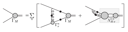
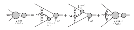
Figure 4: Upper panel: BSE, Eq. (35), which is valid whenever $\Gamma_{\mu}$ can be obtained via a recursion relation. Lower panel: Recursion relation for $\Lambda_{M\nu}^{a;n}$. (Adapted from Ref. detmold .)

Equation (35) is depicted in the upper panel of Fig. 4. The first term is instantly available once one has an explicit form for $\Gamma^{n}_{\nu}$ and the second term, identified by the shaded box in Fig. 4, can be obtained detmold via the inhomogeneous recursion relation depicted in the figure’s lower panel. Combining these figures, it is apparent that to form the Bethe-Salpeter kernel the free gluon line is attached to the upper dressed-quark line. Consequently, the first term on the r.h.s. of the lower panel in Fig. 4 invariably generates crossed gluon lines; viz., nonplanar contributions to the kernel. The character of the vertex-consistent Bethe-Salpeter kernel is now clear: it consists of countably many contributions, a subclass of which are crossed-ladder diagrams and hence nonplanar. Only the rainbow gap equation, obtained with $i=0$ in Eq. (20), yields a planar vertex-consistent Bethe-Salpeter kernel, namely the ladder kernel of Eq. (14). In this case alone is the number of diagrams in the dressed-vertex and kernel identical. Otherwise there are always more terms in the kernel.

Solutions for the $\pi$- and $\rho$-mesons.

I have recapitulated on a general procedure that provides the vertex-consistent channel-projected Bethe-Salpeter kernel once $\Gamma^{n}_{\nu}$ and the propagator functions; $A$, $B$, are known. That kernel must be constructed independently for each channel because, e.g., $\Lambda_{M\nu}^{a}$ depends on $\chi_{M}(q;P)$. As with the study of the vertex, an elucidation of the resulting BSEs’ features is simplified by using the model of Eq. (17), for then the Bethe-Salpeter kernels are finite matrices [cf. $(1-{\cal O})^{-1}$ in Eq. (24)] and the homogeneous BSEs are merely linear, coupled algebraic equations.

Table 1: Calculated $\pi$ and $\rho$ meson masses, in GeV, quoted with ${\cal G}=0.48\,{\rm GeV}$, in which case $m=0.023\,{\cal G}=11\,$MeV. $n$ is the number of dressed-gluon rungs retained in the planar vertex, see Fig. 1, and hence the order of the vertex-consistent Bethe-Salpeter kernel: the rapid convergence of the kernel is apparent from the tabulated results. (Adapted from Ref. detmold .)

	$M_{H}^{n=0}$	$M_{H}^{n=1}$	$M_{H}^{n=2}$	$M_{H}^{n=\infty}$
$\pi$, $m=0$	0	0	0	0
$\pi$, $m=0.011$	0.152	0.152	0.152	0.152
$\rho$, $m=0$	0.678	0.745	0.754	0.754
$\rho$, $m=0.011$	0.695	0.762	0.770	0.770

Reference detmold describes in detail the solution of the coupled gap and Bethe-Salpeter equations for the $\pi$- and $\rho$-mesons. Herein I focus on the results, which are summarised in Table 1. It is evident that, irrespective of the order of the truncation; viz., the number of dressed gluon rungs in the quark-gluon vertex, the pion is massless in the chiral limit. This is in spite of the fact that it is composed of heavy dressed-quarks, as is clear in the calculated scale of the dynamically generated dressed-quark mass function: see Fig. 2, $M(0)\approx{\cal G}\approx 0.5\,$GeV. These observations emphasise that the masslessness of the $\pi$ is a model-independent consequence of consistency between the Bethe-Salpeter kernel and the kernel in the gap equation. Furthermore, the bulk of the $\rho$-$\pi$ mass splitting is present for $m=0$ and with the simplest ($n=0$; i.e., rainbow-ladder) kernel, which demonstrates that this mass difference is driven by the DCSB mechanism. It is not the result of a carefully contrived chromo-hyperfine interaction. Finally, the quantitative effect of improving on the rainbow-ladder truncation; namely, including more dressed-gluon rungs in the gap equation’s kernel and consistently improving the kernel in the Bethe-Salpeter equation, is a 10% correction to the vector meson mass. Simply including the first correction (viz., retaining the first two diagrams in Fig. 1) yields a vector meson mass that differs from the fully resummed result by $\approx 1$%. The rainbow-ladder truncation is clearly accurate in these channels.

Comments.

While I have described results obtained with a rudimentary interaction model in order to make the construction transparent, the procedure is completely general. However, the algebraic simplicity of the analysis is naturally peculiar to the model. With a more realistic interaction, the gap and vertex equations yield a system of twelve coupled integral equations. The Bethe-Salpeter kernel for any given channel then follows as the solution of a determined integral equation.

The material reviewed covers those points in the construction of Refs. truncscheme ; detmold that bear upon the fidelity of the rainbow-ladder truncation in pairing the gap equation and Bethe-Salpeter equations for the vector and flavour non-singlet pseudoscalar mesons. The error is small. In modelling it is therefore justified to fit one’s parameters to physical observables at this level in these channels and then make predictions for other phenomena involving vector and pseudoscalar bound states in the expectation they will be reliable. That approach has been successful, as illustrated in Ref. pieterrev .

Lastly, the placement of the rainbow-ladder truncation as the first term in a procedure that can methodically be improved explains why this truncation has been successful, the boundaries of its success, why it has failed outside these boundaries, and why sorting out the failures won’t undermine the successes.

2.4 Selected Model-Independent Results

In the hadron spectrum the pion is identified as both a Goldstone mode, associated with DCSB, and a bound state composed of constituent $u$- and $d$-quarks, whose effective mass is $\sim 300-500\,$MeV. Naturally, in quantum mechanics, one can fabricate a mass operator that yields a bound state whose mass is much less than the sum of the constituents’ masses. However, that requires fine tuning and, without additional fine tuning, such models predict properties for spin- and/or isospin-flip relatives of the pion which conflict with experiment. A correct resolution of this apparent dichotomy is one of the fundamental challenges to establishing QCD as the theory underlying strong interaction physics, and the DSEs provide an ideal framework within which to achieve that end, as I now explain following the proof of Ref. mrt98 . It cannot be emphasised too strongly that the legitimate understanding of pion observables; including its mass, decay constant and form factors, requires an approach to contain a well-defined and valid chiral limit.

Proof of Goldstone’s Theorem.

Consider the BSE expressed for the isovector pseudoscalar channel:

$$\left[\Gamma_{\pi}^{j}(k;P)\right]_{tu}=\int^{\Lambda}_{q}\,[\chi_{\pi}^{j}(q;P)]_{sr}\,K^{rs}_{tu}(q,k;P)\,,$$ (37)

with $\chi_{\pi}^{j}(q;P)=S(q_{+})\Gamma_{\pi}^{j}(q;P)S(q_{-})$ obvious from Eq. (31) and $j$ labelling isospin, of which the solution has the general form

$$\Gamma_{\pi}^{j}(k;P) = \tau^{j}\gamma_{5}\left[iE_{\pi}(k;P)+\gamma\cdot PF_{\pi}(k;P)\rule{0.0pt}{14.22636pt}\right.$$ (38)

$$\left.\rule{0.0pt}{14.22636pt}+\gamma\cdot k\,k\cdot P\,G_{\pi}(k;P)+\sigma_{\mu\nu}\,k_{\mu}P_{\nu}\,H_{\pi}(k;P)\right].$$

It is apparent that the dressed-quark propagator, the solution of Eq. (1), is an important part of the BSE’s kernel.

Chiral symmetry and its dynamical breaking are expressed in the axial-vector Ward-Takahashi identity, Eq. (10), which involves the axial-vector vertex:

$$\left[\Gamma_{5\mu}^{j}(k;P)\right]_{tu}=Z_{2}\,\left[\gamma_{5}\gamma_{\mu}\frac{\tau^{j}}{2}\right]_{tu}\,+\int^{\Lambda}_{q}\,[\chi_{5\mu}^{j}(q;P)]_{sr}\,K^{rs}_{tu}(q,k;P)\,,$$ (39)

that has the general form

$$\Gamma_{5\mu}^{j}(k;P) = \frac{\tau^{j}}{2}\gamma_{5}\left[\gamma_{\mu}F_{R}(k;P)+\gamma\cdot kk_{\mu}G_{R}(k;P)-\sigma_{\mu\nu}\,k_{\nu}\,H_{R}(k;P)\right]$$ (40)

$$+ \tilde{\Gamma}_{5\mu}^{j}(k;P)+\frac{P_{\mu}}{P^{2}+m_{\phi}^{2}}\phi^{j}(k;P)\,,$$

where $F_{R}$, $G_{R}$, $H_{R}$ and $\tilde{\Gamma}_{5\mu}^{i}$ are regular as $P^{2}\to-m_{\phi}^{2}$, $P_{\mu}\tilde{\Gamma}_{5\mu}^{i}(k;P)\sim{\rm O}(P^{2})$ and $\phi^{j}(k;P)$ has the structure depicted in Eq. (38). Equation (40) admits the possibility of at least one pole term in the vertex but does not require it.

Substituting Eq. (40) into (39) and equating putative pole terms, it is clear that, if present, $\phi^{j}(k;P)$ satisfies Eq. (37). Since this is an eigenvalue problem that only admits a $\Gamma_{\pi}^{j}\neq 0$ solution for $P^{2}=-m_{\pi}^{2}$, it follows that $\phi^{j}(k;P)$ is nonzero solely for $P^{2}=-m_{\pi}^{2}$ and the pole mass is $m_{\phi}^{2}=m_{\pi}^{2}$. Hence, if $K$ supports such a bound state, the axial-vector vertex contains a pion-pole contribution. Its residue, $r_{A}$, however, is not fixed by these arguments. Thus Eq. (40) becomes

$$\Gamma_{5\mu}^{j}(k;P) = \frac{\tau^{j}}{2}\gamma_{5}\left[\gamma_{\mu}F_{R}(k;P)+\gamma\cdot kk_{\mu}G_{R}(k;P)-\sigma_{\mu\nu}\,k_{\nu}\,H_{R}(k;P)\right]$$ (41)

$$+\tilde{\Gamma}_{5\mu}^{i}(k;P)+\frac{r_{A}P_{\mu}}{P^{2}+m_{\pi}^{2}}\Gamma_{\pi}^{j}(k;P)\,.$$

Consider now the chiral limit axial-vector Ward-Takahashi identity, Eq. (10). If one assumes $m_{\pi}^{2}=0$ in Eq. (41), substitutes it into the l.h.s. of Eq. (10) along with Eq. (6) on the right, and equates terms of order $(P_{\nu})^{0}$ and $P_{\nu}$, one obtains the chiral-limit relations mrt98

$$\begin{array}[]{rclcrcl}r_{A}E_{\pi}(k;0)&=&B(k^{2})\,,&&F_{R}(k;0)+2\,r_{A}F_{\pi}(k;0)&=&A(k^{2})\,,\\ G_{R}(k;0)+2\,r_{A}G_{\pi}(k;0)&=&2A^{\prime}(k^{2})\,,&&H_{R}(k;0)+2\,r_{A}H_{\pi}(k;0)&=&0\,.\end{array}$$ (42)

I have already explained that $B(k^{2})\equiv 0$ in the chiral limit [remember Eq. (9)] and that a $B(k^{2})\neq 0$ solution of Eq. (1) in the chiral limit signals DCSB. Indeed, in this case LanePolitzer

$$M(p^{2})\stackrel{{\scriptstyle{\rm large}-p^{2}}}{{=}}\,\frac{2\pi^{2}\gamma_{m}}{3}\,\frac{\left(-\,\langle\bar{q}q\rangle^{0}\right)}{p^{2}\left(\mbox{\footnotesize$\frac{1}{2}$}\ln\left[p^{2}/\Lambda_{\rm QCD}^{2}\right]\right)^{1-\gamma_{m}}}\,,$$ (43)

where $\langle\bar{q}q\rangle^{0}$ is the renormalisation-point-independent vacuum quark condensate bankscasher . Furthermore, there is at least one nonperturbative DSE truncation scheme that preserves the axial-vector Ward-Takahashi identity, order by order. Hence Eqs. (42) are exact quark-level Goldberger-Treiman relations, which state that when chiral symmetry is dynamically broken:

1. the homogeneous isovector pseudoscalar BSE has a massless solution;

2. the Bethe-Salpeter amplitude for the massless bound state has a term proportional to $\gamma_{5}$ alone, with $E_{\pi}(k;0)$ completely determined by the scalar part of the quark self energy, in addition to other pseudoscalar Dirac structures, $F_{\pi}$, $G_{\pi}$ and $H_{\pi}$, that are nonzero;

3. and the axial-vector vertex is dominated by the pion pole for $P^{2}\simeq 0$.

The converse is also true. Hence DCSB is a sufficient and necessary condition for the appearance of a massless pseudoscalar bound state (of what can be very-massive constituents) that dominates the axial-vector vertex for $P^{2}\approx 0$.

Mass Formula.

When chiral symmetry is explicitly broken the axial-vector Ward-Takahashi identity becomes:

$$P_{\mu}\Gamma_{5\mu}^{j}(k;P)=S^{-1}(k_{+})i\gamma_{5}\frac{\tau^{j}}{2}+i\gamma_{5}\frac{\tau^{j}}{2}S^{-1}(k_{-})-2i\,m(\zeta)\,\Gamma_{5}^{j}(k;P),$$ (44)

where the pseudoscalar vertex is obtained from

$$\left[\Gamma_{5}^{j}(k;P)\right]_{tu} = Z_{4}\,\left[\gamma_{5}\frac{\tau^{j}}{2}\right]_{tu}\,+\int^{\Lambda}_{q}\,\left[\chi_{5}^{j}(q;P)\right]_{sr}K^{rs}_{tu}(q,k;P)\,.$$ (45)

As argued in connection with Eq. (39), the solution of Eq. (45) has the form

$$i\Gamma_{5}^{j}(k;P) = \frac{\tau^{j}}{2}\gamma_{5}\left[iE_{R}^{P}(k;P)+\gamma\cdot P\,F_{R}^{P}+\gamma\cdot k\,k\cdot P\,G_{R}^{P}(k;P)\right.$$ (46)

$$\left.+\,\sigma_{\mu\nu}\,k_{\mu}P_{\nu}\,H_{R}^{P}(k;P)\right]+\frac{r_{P}}{P^{2}+m_{\pi}^{2}}\Gamma_{\pi}^{j}(k;P)\,,$$

where $E_{R}^{P}$, $F_{R}^{P}$, $G_{R}^{P}$ and $H_{R}^{P}$ are regular as $P^{2}\to-m_{\pi}^{2}$; i.e., the isovector pseudoscalar vertex also receives a contribution from the pion pole. In this case equating pole terms in the Ward-Takahashi identity, Eq. (44), entails mrt98

$$r_{A}\,m_{\pi}^{2}=2\,m(\zeta)\,r_{P}(\zeta)\,.$$ (47)

This, too, is an exact relation in QCD. Now it is important to determine the residues $r_{A}$ and $r_{P}$.

Study of the renormalised axial-vector vacuum polarisation shows mrt98 :

$$r_{A}\,\delta^{ij}\,P_{\mu}=f_{\pi}\,\delta^{ij}\,P_{\mu} = Z_{2}\,{\rm tr}\int^{\Lambda}_{q}\mbox{\footnotesize$\frac{1}{2}$}\tau^{i}\gamma_{5}\gamma_{\mu}S(q_{+})\Gamma_{\pi}^{j}(q;P)S(q_{-})\,,$$ (48)

where the trace is over colour, Dirac and flavour indices; i.e., the residue of the pion pole in the axial-vector vertex is the pion decay constant. The factor of $Z_{2}$ on the r.h.s. in Eq. (48) is crucial: it ensures the result is gauge invariant, and cutoff and renormalisation-point independent. Equation (48) is the exact expression in quantum field theory for the pseudovector projection of the pion’s wave function on the origin in configuration space.

A close inspection of Eq. (45), following its re-expression in terms of the renormalised, fully-amputated quark-antiquark scattering amplitude: $M=K+K(SS)K+\ldots$, yields mrt98

$$ir_{P}\,\delta^{ij}=Z_{4}\,{\rm tr}\int^{\Lambda}_{q}\mbox{\footnotesize$\frac{1}{2}$}\tau^{i}\gamma_{5}S(q_{+})\Gamma_{\pi}^{j}(q;P)S(q_{-})\,,$$ (49)

wherein the dependence of $Z_{4}$ on the gauge parameter, the regularisation mass-scale and the renormalisation point is exactly that required to ensure: 1) $r_{P}$ is finite in the limit $\Lambda\to\infty$; 2) $r_{P}$ is gauge-parameter independent; and 3) the renormalisation point dependence of $r_{P}$ is just such as to guarantee the r.h.s. of Eq. (47) is renormalisation point independent. Equation (49) expresses the pseudoscalar projection of the pion’s wave function on the origin in configuration space.

Focus for a moment on the chiral limit behaviour of Eq. (49) whereat, using Eqs. (38), (42), one finds readily

$$-\langle\bar{q}q\rangle_{\zeta}^{0}=f_{\pi}r_{P}^{0}(\zeta)=Z_{4}(\zeta,\Lambda)\,N_{c}\,{\rm tr}_{\rm D}\int^{\Lambda}_{q}\!S_{\hat{m}=0}(q)\,.$$ (50)

Equation (50) is unique as the expression for the chiral limit vacuum quark condensate. It is $\zeta$-dependent but independent of the gauge parameter and the regularisation mass-scale, and Eq. (50) thus proves that the chiral-limit residue of the pion pole in the pseudoscalar vertex is  $(-\langle\bar{q}q\rangle_{\zeta}^{0})/f_{\pi}$. Now Eqs. (47), (50) yield

$$(f_{\pi}^{0})^{2}\,m_{\pi}^{2}=-2\,m(\zeta)\,\langle\bar{q}q\rangle_{\zeta}^{0}+{\rm O}(\hat{m}^{2})\,,$$ (51)

where $f_{\pi}^{0}$ is the chiral limit value from Eq. (48). Hence what is commonly known as the Gell-Mann–Oakes–Renner relation is a corollary of Eq. (47).

One can now understand the results in Table 1: a massless bound state of massive constituents is a necessary consequence of DCSB and will emerge in any few-body approach to QCD that employs a systematic truncation scheme which preserves the Ward-Takahashi identities.

Upon review it will be apparent that Eqs. (47) – (49) are valid for any values of the current-quark masses, and the generalisation to $N_{f}$ quark flavours is mr97 ; marisAdelaide ; mishaSVY

$$f_{H}^{2}\,m_{H}^{2}=-\,\langle\bar{q}q\rangle_{\zeta}^{H}{\cal M}_{H}^{\zeta},$$ (52)

${\cal M}^{H}_{\zeta}=m^{\zeta}_{q_{1}}+m^{\zeta}_{q_{2}}$ is the sum of the current-quark masses of the meson’s constituents;

$$f_{H}\,P_{\mu}=Z_{2}\,{\rm tr}\int_{q}^{\Lambda}\!\mbox{\footnotesize$\frac{1}{2}$}(T^{H})^{T}\gamma_{5}\gamma_{\mu}{\cal S}(q_{+})\,\Gamma^{H}(q;P)\,{\cal S}(q_{-})\,,$$ (53)

with ${\cal S}={\rm diag}(S_{u},S_{d},S_{s},\ldots)$, $T^{H}$ a flavour matrix specifying the meson’s quark content, e.g., $T^{\pi^{+}}=\mbox{\footnotesize$\frac{1}{2}$}(\lambda^{1}+i\lambda^{2})$, $\{\lambda^{i}\}$ are $N_{f}$-flavour generalisations of the Gell-Mann matrices; and

$$\langle\bar{q}q\rangle^{H}_{\zeta}=-f_{H}\,r_{H}^{\zeta}=if_{H}\,Z_{4}\,{\rm tr}\int_{q}^{\Lambda}\!\mbox{\footnotesize$\frac{1}{2}$}(T^{H})^{T}\gamma_{5}{\cal S}(q_{+})\,\Gamma^{H}(q;P)\,{\cal S}(q_{-})\,.$$ (54)

NB. Equation (50) means that in the chiral limit $\langle\bar{q}q\rangle^{H}_{\zeta}\to\langle\bar{q}q\rangle_{\zeta}^{0}$ and hence $\langle\bar{q}q\rangle^{H}_{\zeta}$ has been called an in-hadron condensate.

The formulae reviewed in this Section also yield model-independent corollaries for systems involving heavy-quarks, as I relate in Sec. 4.

3 Basis for a Description of Mesons

The renormalisation-group-improved rainbow-ladder truncation has long been employed to study light mesons, and in Secs. 2.2, 2.3 it was shown to be a quantitatively reliable tool for vector and flavour nonsinglet pseudoscalar mesons. In connection with Eqs. (14), (15), I argued that the truncation preserves the ultraviolet behaviour of the quark-antiquark scattering kernel in QCD but requires an assumption about that kernel in the infrared; viz., on the domain $Q^{2}\mathrel{\hbox to0.0pt{\lower 4.0pt\hbox{\hskip 0.0pt$\sim$}\hss}\raise 1.0pt\hbox{$<$}}1\,$GeV², which corresponds to length-scales $\mathrel{\hbox to0.0pt{\lower 4.0pt\hbox{\hskip 0.0pt$\sim$}\hss}\raise 1.0pt\hbox{$>$}}0.2\,$fm. The calculation of this behaviour is a primary challenge in contemporary hadron physics and there is progress raya ; cdrvienna ; latticegluon ; blochmrgluon ; fischer ; latticevertex ; langfeld . However, at present the most efficacious approach is to model the kernel in the infrared, which enables quantitative comparisons with experiments that can be used to inform theoretical analyses. The most extensively applied model is specified by pmspectra2

$$\frac{\alpha(Q^{2})}{Q^{2}}=\frac{4\pi^{2}}{\omega^{6}}D\,Q^{2}{\rm e}^{-Q^{2}/\omega^{2}}+\,\frac{8\pi^{2}\,\gamma_{m}}{\ln\left[\tau+\left(1+Q^{2}/\Lambda_{\rm QCD}^{2}\right)^{2}\right]}\,{\cal F}(Q^{2})\,,$$ (55)

in Eqs. (14), (15). Here, ${\cal F}(Q^{2})=[1-\exp(-Q^{2}/[4m_{t}^{2}])]/Q^{2}$, $m_{t}$ $=$ $0.5\,$GeV; $\tau={\rm e}^{2}-1$; $\gamma_{m}=12/25$; and pdg98 $\Lambda_{\rm QCD}=\Lambda^{(4)}_{\overline{\rm MS}}=0.234\,$GeV. This simple form expresses the interaction strength as a sum of two terms: the second ensures that perturbative behaviour is preserved at short-range; and the first makes provision for the possibility of enhancement at long-range. The true parameters in Eq. (55) are $D$ and $\omega$, which together determine the integrated infrared strength of the rainbow-ladder kernel; i.e., the so-called interaction tension, $\sigma^{\Delta}$ cdrvienna . However, I emphasise that they are not independent: in fitting to a selection of observables, a change in one is compensated by altering the other; e.g., on the domain $\omega\in[0.3,0.5]\,$GeV, the fitted observables are approximately constant along the trajectory raya

$$\omega\,D=(0.72\,{\rm GeV})^{3}.$$ (56)

Hence Eq. (55) is a one-parameter model. This correlation: a reduction in $D$ compensating an increase in $\omega$, ensures a fixed value of the interaction tension.

3.1 Rainbow Gap Equation

Equations (15) and (55) provide a model for QCD’s gap equation and in hadron physics applications one is naturally interested in the nonperturbative DCSB solution. A familiar property of gap equations is that they only support such a solution if the interaction tension exceeds some critical value. In the present case that value is $\sigma_{c}^{\Delta}\sim 2.5\,$GeV/fm cdrvienna . This amount of infrared strength is sufficient to generate a nonzero vacuum quark condensate but only just. An acceptable description of hadrons requires $\sigma^{\Delta}\sim 25\,$GeV/fm mr97 and that is obtained with pmspectra2

$$D=(0.96\,{\rm GeV})^{2}\,.$$ (57)

This value of the model’s infrared mass-scale parameter and the two current-quark masses

$$\begin{array}[]{cc}m_{u}(1\,{\rm GeV})=5.5\,{\rm MeV}\,,&m_{s}(1\,{\rm GeV})=125\,{\rm MeV}\,,\end{array}$$ (58)

defined using the one-loop expression

$$\frac{m(\zeta)}{m(\zeta^{\prime})}=Z_{m}(\zeta^{\prime},\zeta)\stackrel{{\scriptstyle\rm 1-loop}}{{=}}\left(\frac{\ln[\zeta^{\prime}/\Lambda_{\rm QCD}]}{\ln[\zeta/\Lambda_{\rm QCD}]}\right)^{\gamma_{m}}$$ (59)

to evolve $m_{u}(19\,{\rm GeV})=3.7\,$MeV and $m_{s}(19\,{\rm GeV})=85\,$MeV, were obtained in Ref. pmspectra2 by requiring a least-squares fit to the $\pi$- and $K$-meson observables listed in Table 2. The procedure was straightforward: the rainbow gap equation [Eqs. (7), (15), (55)] was solved with a given parameter set and the output used to complete the kernels in the homogeneous ladder BSEs for the $\pi$- and $K$-mesons [Eqs. (14), (15), (37), (38) with $\tau^{j}$ for the $\pi$ channel and $\tau^{j}\to T^{K^{+}}=\mbox{\footnotesize$\frac{1}{2}$}(\lambda^{4}+i\lambda^{5})$ for the $K$]. These BSEs were solved to obtain the $\pi$- and $K$-meson masses, and the Bethe-Salpeter amplitudes. Combining this information delivers the leptonic decay constants via Eq. (53). This was repeated as necessary to arrive at the results in Table 2. The model gives a vacuum quark condensate

$$-\langle\bar{q}q\rangle^{0}_{1\,{\rm GeV}}=(0.242\,{\rm GeV})^{3}\,,$$ (60)

calculated from Eq. (50) and evolved using the one-loop expression in Eq. (59).

Table 2: Comparison of experimental values with results for $\pi$ and $K$ observables calculated using the rainbow-ladder interaction specified by Eq. (55), quoted in MeV. The model’s sole parameter and the current-quark masses were varied to obtain these results, and the best fit parameter values are given in Eqs. (57), (58). Predictions for analogous vector meson observables are also tabulated. NB. A charged particle normalisation is used for $f_{H}^{V}$ in Eq. (61), which differs from that in Eq. (53) by a multiplicative factor of $\surd 2$. (Adapted from Ref. pmspectra2 .)

	$m_{\pi}$	$m_{K}$	$f_{\pi}$	$f_{K}$	$m_{\rho}$	$m_{K^{\ast}}$	$m_{\phi}$	$f_{\rho}$	$f_{K^{\ast}}$	$f_{\phi}$
Calc. pmspectra2	138	497	93	109	742	936	1072	207	241	259
Expt. pdg98	138	496	92	113	771	892	1019	217	227	228
Rel. Error					0.04	-0.05	-0.05	0.05	-0.06	-0.14

With the model’s single parameter fixed, and the dressed-quark propagator determined, it is straightforward to compose and solve the homogeneous BSE for vector mesons. This yields predictions, also listed in Table 2, for the vector meson masses and electroweak decay constants mishaSVY

$$f_{H}^{V}\,M_{H}^{V}=\mbox{\footnotesize$\frac{1}{3}$}Z_{2}\,{\rm tr}\int_{q}^{\Lambda}\!(T^{H})^{T}\gamma_{\mu}\,{\cal S}(q_{+})\,\Gamma_{\mu}^{H}(q;P)\,{\cal S}(q_{-})\,,$$ (61)

where $M_{H}^{V}$ is the meson’s mass and $P_{\mu}\Gamma_{\mu}^{H}(q;P)=0$ for $P^{2}=-(M_{V}^{H})^{2}$; i.e., the Bethe-Salpeter amplitude is transverse. $f_{H}^{V}$ characterises decays such as $\rho\to e^{+}e^{-}$, $\tau\to K^{\ast}\nu_{\tau}$.

Given the discussion in Sec. 2, the phenomenological success of the rainbow-ladder kernel, manifest in the results of Table 2, is unsurprising and, indeed, was to be expected.

3.2 Comparison with Lattice Simulations

The solution of the gap equation has long been of interest in grappling with DCSB in QCD and hence, in Figs. 5, I depict the scalar functions characterising the renormalised dressed-quark propagator: the wave function renormalisation, $Z(p^{2})$, and mass function, $M(p^{2})$, obtained by solving Eq. (15) using Eq. (55). The infrared suppression of $Z(p^{2})$ and enhancement of $M(p^{2})$ are longstanding predictions of DSE studies cdragw . Indeed, this property of asymptotically free theories was elucidated in Refs. LanePolitzer and could be anticipated from studies of strong coupling QED bjw . The prediction has recently been confirmed in numerical simulations of quenched lattice-QCD, as is evident in the figures.

Figure 5: Left panel – wave function renormalisation: solution of the gap equation using Eqs. (55), (57) (solid curve); solution using Eqs. (55), (62) (dashed-curve); quenched lattice-QCD simulations latticequark , obtained with $m=0.036/a\sim 60\,$MeV (data). The DSE study used a renormalisation point $\zeta=19\,$GeV and a current-quark mass $0.6\,m_{s}^{1\,{\rm GeV}}$ [Eq. (58)], to enable a direct comparison with the lattice data. Right panel – mass function. (Adapted from Ref. raya .)

It is not yet possible to reliably determine the behaviour of lattice Schwinger functions for current-quark masses that are a realistic approximation to those of the $u$- and $d$-quarks. A veracious lattice estimate of $m_{\pi}$, $f_{\pi}$, $\langle\bar{q}q\rangle^{0}$ is therefore absent. To obtain such an estimate, Ref. raya used the rainbow kernel described herein and varied $(D,\omega)$ in order to reproduce the quenched lattice-QCD data. A best fit was obtained with

$$\begin{array}[]{cc}D=(0.74\,{\rm GeV})^{2}\,,&\omega=0.3\,{\rm GeV}\,,\end{array}$$ (62)

at a current-quark mass of $0.6\,m_{s}^{1\,{\rm GeV}}\!\approx 14\,m_{u}$ [Eq. (58)] chosen to coincide with that employed in the lattice simulation. Constructing and solving the homogeneous BSE for a pion-like bound state composed of quarks with this current-mass yields

$$m_{\pi}^{m_{q}\sim 14m_{u}}=0.48\,{\rm GeV},\;f_{\pi}^{m_{q}\sim 14m_{u}}=0.094\,{\rm GeV}\,.$$ (63)

The parameters in Eq. (62) give chiral limit results raya :

$$f_{\pi}^{0}=0.068\,{\rm GeV}\,,\;-\langle\bar{q}q\rangle^{0}_{1\,{\rm GeV}}=(0.19\,{\rm GeV})^{3}\,,$$ (64)

whereas Eqs. (56), (57) give $f_{\pi}^{0}=0.088\,$GeV. These results have been confirmed in a more detailed analysis mandarlattice and this correspondence suggests that chiral and physical pion observables are materially underestimated in the quenched theory: $|\langle\bar{q}q\rangle|$ by a factor of two and $f_{\pi}$ by $30$%.

The rainbow-ladder kernel has also been employed in an analysis of a trajectory of fictitious pseudoscalar mesons, all composed of equally massive constituents pmqciv (The only physical state on this trajectory is the pion.) The DSE study predicts cdrqciv

$$\frac{m_{H_{m=2m_{s}}}}{m_{H_{m=m_{s}}}}=2.2\,,$$ (65)

in agreement with a result of recent quenched lattice simulations michaels . The DSE study provides an intuitive understanding of this result, showing that it owes itself to a large value of the in-hadron condensates for light-quark mesons; e.g., $\langle\bar{q}q\rangle^{s\bar{s}}_{1\,{\rm GeV}}=(-0.32\,{\rm GeV})^{3}$ mr97 , and thereby confirms the large-magnitude condensate version of chiral perturbation theory, an observation also supported by Eq. (64). References pmqciv ; TandyErice also provide vector meson trajectories.

3.3 Ab Initio Calculation of Meson Properties

The renormalisation-group-improved rainbow-ladder kernel defined with Eq. (55) has been employed to predict a wide range of meson observables, and this is reviewed in Ref. pieterrev . These results; e.g., those for vector mesons in Table 2, are true predictions, in the sense that the model’s mass-scale was fixed, as described in connection with Eq. (57), and every element in each calculation was completely determined by, and calculated from, that kernel.

A particular success was the calculation of the electromagnetic pion form factor, which is described in Refs. pieterpion ; pieterpiK . The result is depicted in Fig. 6, wherein it is compared with the most recent experimental data Volmer:2000ek . It is noteworthy that all other pre-existing calculations are uniformly two – four standard deviations below that $Q^{2}F_{\pi}(Q^{2})$ data.

In this connection one should also note that it is a model independent DSE prediction Maris:1998hc that electromagnetic elastic meson form factors display

$$q^{2}F(q^{2})={\rm constant},\;q^{2}\gg\Lambda_{\rm QCD}^{2},$$ (66)

with calculable $(\ln q^{2}/\Lambda_{\rm QCD}^{2})^{d}$ corrections, where $d$ is an anomalous dimension. This agrees with earlier perturbative QCD analyses Farrar:1979aw ; Lepage:1980fj . However, to obtain this result in covariant gauges it is crucial to retain the pseudovector components of the Bethe-Salpeter amplitude in Eq. (38): $F_{\pi}$, $G_{\pi}$. (NB. The quark-level Goldberger-Treiman relations, Eqs. (42), prove them to be nonzero.) Without these amplitudes cdrpion , $q^{2}F(q^{2})\propto 1/q^{2}$. The calculation of Ref. Maris:1998hc suggests that the perturbative behaviour of Eq. (66) is unambiguously evident for $q^{2}\mathrel{\hbox to0.0pt{\lower 4.0pt\hbox{\hskip 0.0pt$\sim$}\hss}\raise 1.0pt\hbox{$>$}}15\,$GeV². Owing to challenges in the numerical analysis, the ab initio calculations of Ref. pieterpiK cannot yet make a prediction for the onset of the perturbative domain but progress in remedying that is being made pichowskypoles .

Another very instructive success is the study of $\pi$-$\pi$ scattering, wherein a range of new challenges arise whose quiddity and natural resolution via a symmetry-preserving truncation of the DSEs is explained in Sec. 4.6 of Ref. pieterrev , which reviews the seminal work of Refs. bicudo . It is worth remarking, too, that with a systematic and nonperturbative DSE truncation scheme, all consequences of the Abelian anomaly and Wess-Zumino term are obtained exactly, without fine tuning cdrpion ; Maris:1998hc ; WZterm ; bando ; racdr ; Maris:2002mz .

Figure 6: Impulse approximation DSE prediction for $q^{2}F_{\pi}(q^{2})$ obtained in a parameter-free application of the renormalisation-group-improved rainbow-ladder truncation, Eqs. (55), (57). The data are from Refs. Brauel:1979zk ; Amendolia:1986wj ; Volmer:2000ek . (Adapted from Ref. Maris:2001am .)

3.4 Heavier Mesons

The meson spectrum contains pdg98 four little-studied axial-vector mesons composed of $u$- and $d$-quarks. They appear as isospin $I=0,1$ partners (in the manner of the $\omega$ and $\rho$): $h_{1}(1170)$, $b_{1}(1235)$; and $f_{1}(1285)$, $a_{1}(1260)$, and differ in their charge-parity: $J^{PC}=1^{+-}$ for $h_{1}$, $b_{1}$; and $J^{PC}=1^{++}$ for $f_{1}$, $a_{1}$. In the $q\bar{q}$ constituent quark model the $b_{1}$ is represented as a constituent-quark and -antiquark with total spin $S=0$ and angular momentum $L=1$, while in the $a_{1}$ the quark and antiquark have $S=1$ and $L=1$. It is therefore apparent that in this model the $b_{1}$ is an orbital excitation of the $\pi$, and the $a_{1}$ is an orbital excitation and axial-vector partner of the $\rho$. In QCD the $J^{PC}$ characteristics of a quark-antiquark bound state are manifest in the structure of its Bethe-Salpeter amplitude llewellyn . This amplitude is a valuable intuitive guide and, in cases where a $q\bar{q}$ constituent quark model analogue exists, it incorporates and extends the information present in that analogue’s quantum mechanical wave function.

Three of the axial-vector mesons decay predominantly into two-body final states containing a vector meson and a pion: $h_{1}\to\rho\pi$; $b_{1}\to\omega\pi$; $a_{1}\to\rho\pi$. With a $J=1$ meson in both the initial and final state these three decays proceed via two partial waves ($S$, $D$), and therefore probe aspects of hadron structure inaccessible in simpler processes involving only spinless mesons in the final state, such as $\rho\to\pi\pi$. For example and of importance, in constituent-quark-like models the $D/S$ amplitude ratio is very sensitive eric to the nature of the phenomenological long-range confining interaction.

The additional insight and model constraints that such processes can provide is particularly important now as a systematic search and classification of “exotic” states in the light meson sector becomes feasible experimentally. I note that a meson is labelled “exotic” if it is characterised by a value of $J^{PC}$ which is unobtainable in the $q\bar{q}$ constituent quark model; e.g., the experimentally observed exotic $\pi_{1}(1600)$, a $1.6\,$GeV $J^{PC}=1^{-+}$ state. Such unusual charge parity states are a necessary feature of a field theoretical description of quark-antiquark bound states llewellyn with BSE studies typically yielding bsesep masses approximately twice as large as that of the natural charge parity partner and, in particular, a $J^{PC}=1^{-+}$ meson with a mass $\sim 1.5\,$GeV bpprivate .

In appreciation of these points, Ref. a1b1 used the simple DSE-based model of Ref. bsesep in a simultaneous study of axial-vector meson decays, $\rho\to\pi\pi$ decay, and the electroweak decay constants of the mesons involved. The results are instructive. It was found that the rainbow-ladder truncation is capable of simultaneously providing a good description of these observables but that the $D/S$ partial-wave ratio in the decays of axial-vector mesons is indeed very sensitive to details of the long-range part of a model interaction; i.e., to the expression of light-quark confinement. This is perhaps unsurprising given that the mass of each axial-vector meson mass is significantly greater than $2M(0)$; namely, twice the constituent-quark mass-scale. Unfortunately, more sophisticated calculations are lacking. This collection of experimentally well-understood mesons has many lessons to teach and should no longer be ignored.

4 Heavy Quarks

4.1 Features of the Mass Function

The DSE methods described hitherto have been applied to mesons involving heavy-quarks mishaSVY ; misha1 ; misha2 and in this case there is a natural simplification. To begin, one focuses on the fact that mesons, whether heavy or light, are bound states of a dressed-quark and -antiquark, with the dressing described by the gap equation, Eq. (1), written explicitly again here with the addition of flavour label, $f\,(=u,d,s,c,b)$:

$$S_{f}(p)^{-1}=i\gamma\cdot p\,A_{f}(p^{2})+B_{f}(p^{2})=A_{f}(p^{2})\left[i\gamma\cdot p+M_{f}(p^{2})\right]$$ (67)

$$= Z_{2}(i\gamma\cdot p+m_{f}^{\rm bm})+\,Z_{1}\int^{\Lambda}_{q}\!g^{2}D_{\mu\nu}(p-q)\frac{\lambda^{a}}{2}\gamma_{\mu}S_{f}(q)\Gamma^{fa}_{\nu}(q,p)\,.$$ (68)

The other elements of Eq. (68) will already be familiar.

The qualitative features of the gap equation’s solution are known and typical mass functions, $M_{f}(p^{2})$, are depicted in Fig. 7. There is some quantitative model-dependence in the momentum-evolution of the mass-function into the infrared. However, with any Ansatz for the effective interaction that provides an accurate description of $f_{\pi,K}$ and $m_{\pi,K}$, one obtains solutions with profiles like those illustrated in the figure. Owing to Eq. (13) the ultraviolet behaviour is naturally fixed, namely, it is given by Eq. (5) for massive quarks and by Eq. (43) in the chiral limit.

Figure 7: Quark mass function obtained as a solution of Eq. (67) using the rainbow truncation, discussed in connection with Eqs. (12) – (15), and the interaction of Eq. (55) with current-quark masses, fixed at $\zeta=19\,$GeV: $m_{u,d}(\zeta)=3.7\,$MeV, $m_{s}(\zeta)=82\,$MeV, $m_{c}(\zeta)=0.58\,$GeV and $m_{b}(\zeta)=3.8\,$GeV. The indicated solutions of $M^{2}(p^{2})=p^{2}$ define a Euclidean constituent-quark mass, $M^{E}_{f}$, which takes the values: $M^{E}_{u}=0.56\,$GeV, $M^{E}_{s}=0.70\,$GeV, $M^{E}_{c}=1.3\,$GeV, $M^{E}_{b}=4.6\,$GeV.

It is apparent in the figure that as $p^{2}$ decreases the chiral-limit and $u,d$-quark mass functions evolve to coincidence. This feature signals a transition from the perturbative to the nonperturbative domain. Furthermore, since the chiral limit mass-function is nonzero only because of the nonperturbative DCSB mechanism, whereas the $u,d$-quark mass function is purely perturbative at $p^{2}>20\,$GeV², it also indicates clearly that the DCSB mechanism has a significant impact on the propagation characteristics of $u,d,s$-quarks. However, it is conspicuous in Fig. 7 that this is not the case for the $b$-quark. Its large current-quark mass almost entirely suppresses momentum-dependent dressing so that $M_{b}(p^{2})$ is nearly constant on a substantial domain. The same is true to a lesser extent for the $c$-quark.

The quantity ${\cal L}_{f}:=M^{E}_{f}/m_{f}(\zeta)$ provides a single quantitative measure of the importance of the DCSB mechanism; i.e., nonperturbative effects, in modifying the propagation characteristics of a given quark flavour. In this particular illustration it takes the values

$$\begin{array}[]{c|ccccc}f&u,d&s&c&b\\ \hline\cr{\cal L}_{f}&150&10&2.2&1.2\end{array}\,,$$ (69)

which are representative: for light-quarks ${\cal L}_{q=u,d,s}\sim 10$-$100$; while for heavy-quarks ${\cal L}_{Q=c,b}\sim 1$. They also highlight the existence of a mass-scale, $M_{\chi}$, characteristic of DCSB: the propagation characteristics of a flavour with $m_{f}(\zeta)\leq M_{\chi}$ are significantly altered by the DCSB mechanism, while momentum-dependent dressing is almost irrelevant for flavours with $m_{f}(\zeta)\gg M_{\chi}$. It is evident and unsurprising that $M_{\chi}\sim 0.2\,$GeV$\,\sim\Lambda_{\rm QCD}$. Consequently one anticipates that the propagation of $c,b$-quarks should be described well by replacing their mass-functions with a constant; viz., writing mishaSVY

$$S_{Q}(p)=\frac{1}{i\gamma\cdot p+\hat{M}_{Q}}\,,\;Q=c,b\,,$$ (70)

where $\hat{M}_{Q}$ is a constituent-heavy-quark mass parameter.

When considering a meson with an heavy-quark constituent one can proceed further, as in heavy-quark effective theory (HQET) neubert94 , allow the heaviest quark to carry all the heavy-meson’s momentum: $P_{\mu}=:m_{H}v_{\mu}=:(\hat{M}_{Q}+E_{H})v_{\mu}$, and write

$$S_{Q}(k+P)=\frac{1}{2}\,\frac{1-i\gamma\cdot v}{k\cdot v-E_{H}}+{\rm O}\left(\frac{|k|}{\hat{M}_{Q}},\frac{E_{H}}{\hat{M}_{Q}}\right)\,,$$ (71)

where $k$ is the momentum of the lighter constituent. It is apparent from the study of light-meson properties that in the calculation of observables the meson’s Bethe-Salpeter amplitude will limit the range of $|k|$ so that Eq. (71) will only be a good approximation if both the momentum-space width of the amplitude, $\omega_{H}$, and the binding energy, $E_{H}$, are significantly less than $\hat{M}_{Q}$.

In Ref. misha2 the propagation of $c$- and $b$-quarks was described by Eq. (71), with a goal of exploring the fidelity of this idealisation, and it was found to allow for a uniformly good description of $B_{f}$-meson leptonic and semileptonic decays with heavy- and light-pseudoscalar final states. In that study, $\omega_{B_{f}}\approx 1.3\,$GeV and $E_{B_{f}}\approx 0.70\,$GeV, both of which are small compared with $\hat{M}_{b}\approx 4.6\,$GeV in Fig. 7. Hence the accuracy of the approximation could be forseen. It is reasonable to suppose that $\omega_{D}\approx\omega_{B}$ and $E_{D}\approx E_{B}$, since they must be identical in the limit of exact heavy-quark symmetry. Thus in processes involving the weak decay of a $c$-quark ($\hat{M}_{c}\approx 1.3\,$GeV) where a $D_{f}$-meson is the heaviest participant, Eq. (71) must be inadequate; an expectation verified in Ref. misha2 .

The failure of Eq. (71) for the $c$-quark complicates or precludes the development of a common understanding of $D_{f}$- and $B_{f}$-meson observables using such contemporary theoretical tools as HQET and light cone sum rules. However, as shown in Ref. mishaSVY and I will illustrate, the constituent-like dressed-heavy-quark propagator of Eq. (70) can still be used to effect a unified, accurate simplification in the study of these observables.

4.2 Leptonic Decays

Pseudoscalar Mesons.

The leptonic decay of a pseudoscalar meson, $P(p)$, is described by the matrix element (Sec. 2.4)

$$f_{P}\,p_{\mu}:=\langle 0|\bar{\cal Q}\,(T^{P})^{\rm T}\gamma_{\mu}\gamma_{5}\,{\cal Q}|P(p)\rangle={\rm tr}\,Z_{2}\int^{\Lambda}_{k}\,(T^{P})^{\rm T}\gamma_{5}\gamma_{\mu}\,\chi_{P}(k;p),$$ (72)

where ${\cal Q}={\rm column}(u,d,s,c,b)$ and here I have adopted a charged particle normalisation, which yields results for $f_{P}$ a factor of $\surd 2$ larger than Eq. (53) and is conventional in studying heavy-quark systems.

In Eq. (72), $\chi_{P}$ is the meson’s Bethe-Salpeter wave function, related to its amplitude, $\Gamma_{P}$, via Eq. (31) and normalised canonically as described in connection with Eq. (30). Using Eq. (71), it follows from the canonical normalisation condition that

$${\cal G}_{P}(k;p):=\frac{1}{\surd m_{P}}\,\Gamma_{P}(k;p)<\infty\,,\;m_{P}\to\infty\,;$$ (73)

i.e., ${\cal G}_{P}(k;p)$ so-defined is mass-independent in the heavy-quark limit. Using this result plus Eq. (71) one finds from Eq. (72) misha1

$$f_{P}\propto\frac{1}{\surd{m_{P}}}\,,\;m_{P}\to\infty\,.$$ (74)

Equation (74) is a model-independent result and a well-known general consequence of heavy-quark symmetry neubert94 . However, the value of the hadron mass at which this behaviour becomes evident is unknown. It is clear from Table 2 that, experimentally,

$$f_{\pi}=131\,{\rm MeV}\;<\;f_{K}=160\,{\rm MeV}.$$ (75)

Furthermore, direct DSE studies following the method described in Sec. 3.3 show that for pseudoscalar mesons $u\bar{f}$, composed of a single $u,d$-quark and an antiquark of mass $m_{f}$, $f_{P}(m_{P})$ is a monotonically increasing concave-down function on $m_{P}\in[0,0.9]\,{\rm GeV}$, where $m_{P}$ is the calculated mass of this composite system, and likely on a larger domain TandyErice . On the other hand, numerical simulations of quenched lattice-QCD indicate flynn

$$f_{D}=200\pm 30\,{\rm MeV}\;>\;f_{B}=170\pm 35\,{\rm MeV}\,.$$ (76)

In simulations of lattice-QCD with two flavours of sea quarks both of these decay constants increase in magnitude but there is no sign that the ordering is reversed flynn ; mcneile . The information in Eqs. (75), (76) is depicted in Fig. 8. This and analysis to be reviewed subsequently suggest that D-mesons lie outside the domain on which Eq. (74) is a reliable tool.

Vector Mesons.

The leptonic decay constant, $f_{V}$, for a vector meson with mass $M_{V}$ is given in Eq. (61) and adapting the analysis that leads to Eq. (74) one finds readily

$$f_{V}\propto\frac{1}{\sqrt{M_{V}}}\,,\;M_{V}\to\infty\,,$$ (77)

which again is a model-independent result. Moreover, since the pseudoscalar and vector meson Bethe-Salpeter amplitudes become identical in the heavy-quark limit, it follows that mishaSVY

$$f_{V}=f_{P}\,,\;M_{V}=m_{P}\,,\;\mbox{\rm in the limit}\;m_{P}\to\infty\,.$$ (78)

Figure 8: Experimental values of $f_{\pi,K}$ (Eq. (75), filled circles); lattice estimates of $f_{D,B}$ (Eq. (76), open circles); values of $f_{\pi,K,D,B}$ calculated in Ref. mishaSVY (open diamonds). Least-squares fit to the experimental values and lattice estimates (dashed curve): $f_{P}^{2}=(0.013+0.028\,m_{P})/(1+0.055\,m_{P}+0.15\,m_{P}^{2})$, which exhibits the large-$m_{P}$ limit of Eq. (74); the large-$m_{P}$ limit of this fit (dot-dashed curve). (Adapted from Ref. mishaSVY .)

4.3 Heavy-Meson Masses

More can be learnt from the pseudoscalar meson mass formula in Eq. (52). Using Eq. (74), and applying to Eq. (54) the analysis from which it follows, one obtains

$$-\langle\bar{q}q\rangle^{P}_{\zeta}=\mbox{constant}\,,\;\mbox{as~{}}m_{P}\to\infty$$ (79)

and consequently marisAdelaide ; mishaSVY

$$m_{P}\propto\hat{m}_{Q}\,,\;\hat{m}_{Q}\to\infty\,,$$ (80)

where $\hat{m}_{Q}$ is the renormalisation-group-invariant current-quark mass of the flavour-nonsinglet pseudoscalar meson’s heaviest constituent. This is the result one would have guessed from constituent-quark models but here I have outlined a direct proof in QCD.

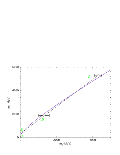
Figure 9: Pseudoscalar $u\bar{q}$ meson’s mass as a function of $m_{q}({\zeta})$, $\zeta=19\,{\rm GeV}$, with a fixed value of $m_{u}({\zeta})$ corresponding to $m_{u}(1\,{\rm GeV})=5.5\,$MeV, Eq. (58) (solid line). The experimental data points are from Ref. pdg98 as are the errors assigned to the associated heavy-quark masses. A straight line is drawn through the $K$, $D$, $B$ masses (dashed curve). (Adapted from Ref. cdrlc01 . See also Ref. TandyErice .)

Equation (47) is thus seen to be a single formula that unifies the masses of light- and heavy-quark mesons. This aspect has been quantitatively explored using the rainbow-ladder kernel described in Sec. 3, with the results illustrated in Fig. 9. Therein the calculated mass of a $u\bar{f}$ pseudoscalar meson is plotted as a function of $m_{f}(\zeta)$, with $m_{u}(\zeta)$ fixed at the value in Eq. (58). The DSE calculations are depicted by the solid curve, which is pmqciv (in MeV)

$$m_{P}=83+500\sqrt{\cal X}+310\,{\cal X},\;{\cal X}=m_{q}^{\zeta}/\Lambda_{\rm QCD}.$$ (81)

The curvature appears slight in the figure but that is misleading: the nonlinear term in Eq. (81) accounts for almost all of $m_{\pi}$ (the Gell-Mann–Oakes-Renner relation is nearly exact for the pion) and $80\,$% of $m_{K}$. NB. The dashed line in Fig. 9 fits the $K$, $D$, $B$ subset of the data exactly. It is drawn to illustrate how easily one can be misled. Without careful calculation one might infer from this apparent agreement that the large-$m_{q}$ limit of Eq. (47) is already manifest at the $s$-quark mass whereas, in reality, the linear term only becomes dominant for $m_{q}\mathrel{\hbox to0.0pt{\lower 4.0pt\hbox{\hskip 0.0pt$\sim$}\hss}\raise 1.0pt\hbox{$>$}}1\,$GeV, providing $50\,$% of $m_{D}$ and $67\,$% of $m_{B}$. The model predicts, via Eq. (59), $m_{c}^{1\,{\rm GeV}}=1.1\,$GeV and $m_{b}^{1\,{\rm GeV}}=4.2\,$GeV, values that are typical of Poincaré covariant treatments.

4.4 Semileptonic Transition Form Factors

Pseudoscalar meson in the final state.

The transition: $P_{1}(p_{1})\to P_{2}(p_{2})\,\ell\,\nu\,,$ where $P_{1}$ represents either a $B$- or $D$-meson and $P_{2}$ can be a $D$, $K$ or $\pi$, is described by the invariant amplitude

$$A(P_{1}\to P_{2}\,\ell\,\nu)=\frac{G_{F}}{\surd 2}\,V_{f^{\prime}f}\;\bar{\ell}\,\gamma_{\mu}(1-\gamma_{5})\nu\;M_{\mu}^{P_{1}P_{2}}(p_{1},p_{2})\,,$$ (82)

where $G_{F}=1.166\times 10^{-5}\,$GeV^-2, $V_{f^{\prime}f}$ is the relevant element of the Cabibbo-Kobayashi-Maskawa (CKM) matrix, and the hadronic current is

$$M_{\mu}^{P_{1}P_{2}}(p_{1},p_{2}) := \langle P_{2}(p_{2})|\bar{f}^{\prime}\gamma_{\mu}f|P_{1}(p_{1})\rangle=f_{+}(t)\,(p_{1}+p_{2})_{\mu}+f_{-}(t)\,q_{\mu}\,,$$ (83)

with $t:=-q^{2}=-(p_{1}-p_{2})^{2}$. The transition form factors, $f_{\pm}(t)$, contain all the information about strong-interaction effects in these processes, and their accurate calculation is essential for a reliable determination of the CKM matrix elements from a measurement of the decay width ($t_{\pm}:=(m_{P_{1}}\pm m_{P_{2}})^{2}$):

$$\Gamma(P_{1}\to P_{2}\ell\nu)=\frac{G_{F}^{2}}{192\pi^{3}}\,|V_{f^{\prime}f}|^{2}\,\frac{1}{m_{P_{1}}^{3}}\,\int_{0}^{t_{-}}\,dt\,|f_{+}(t)|^{2}\,\left[(t_{+}-t)(t_{-}-t)\right]^{3/2}\!\!.$$ (84)

The related study of light-meson initial states is described in Refs. mitchell .

Vector meson in the final state.

The transition: $P(p_{1})\to V_{\lambda}(p_{2})\,\ell\,\nu\,,$ with $P$ either a $B$ or $D$ and $V_{\lambda}$ a $D^{\ast}$, $K^{\ast}$ or $\rho$, is described by the invariant amplitude

$$A(P\to V_{\lambda}\,\ell\,\nu)=\frac{G_{F}}{\surd 2}\,V_{f^{\prime}f}\,\bar{\ell}\,i\gamma_{\mu}(1-\gamma_{5})\nu\,\epsilon_{\nu}^{\lambda}(p_{2})\,M_{\mu\nu}^{PV_{\lambda}}(p_{1},p_{2})\,,$$ (85)

in which the hadronic tensor involves four scalar functions

$$\epsilon_{\nu}^{\lambda}(p_{2})\,M_{\mu\nu}^{PV_{\lambda}}(p_{1},p_{2}) = \epsilon_{\mu}^{\lambda}\,(m_{P}+M_{V})\,A_{1}(t)+(p_{1}+p_{2})_{\mu}\,\epsilon^{\lambda}\cdot q\,\frac{A_{2}(t)}{m_{P}+M_{V}}$$

$$+ q_{\mu}\,\epsilon^{\lambda}\cdot q\,\frac{A_{3}(t)}{m_{P}+M_{V}}\,+\,\varepsilon_{\mu\nu\alpha\beta}\,\epsilon_{\nu}^{\lambda}\,p_{1\alpha}\,p_{2\beta}\,\frac{2V(t)}{m_{P}+M_{V}}\,.$$

Introducing three helicity amplitudes

$$H_{\pm} = (m_{P}+M_{V})\,A_{1}(t)\,\mp\,\frac{\lambda^{\frac{1}{2}}(m_{P}^{2},M_{V}^{2},t)}{m_{P}+M_{V}}\,V(t)\,,$$ (87)

$$H_{0} = \frac{1}{2\,M_{V}\surd t}\left(\left[m_{P}^{2}-M_{V}^{2}-t\right]\,\left[m_{P}+M_{V}\right]A_{1}(t)-\frac{\lambda(m_{P}^{2},M_{V}^{2},t)}{m_{P}+M_{V}}\,A_{2}(t)\right)\!,$$

where $\lambda(m_{P}^{2},M_{V}^{2},t)=[t_{+}-t]\,[t_{-}-t]$, $t_{\pm}=(m_{P}\pm M_{V})^{2}$, the transition rates

$$\frac{d\Gamma_{\pm,0}}{dt} = \frac{G_{F}^{2}}{192\pi^{3}m_{P_{1}}^{3}}\,|V_{f^{\prime}f}|^{2}\,t\,\lambda^{\frac{1}{2}}(m_{P}^{2},M_{V}^{2},t)\,|H_{\pm,0}(t)|^{2}\,,$$ (89)

from which one obtains the transverse and longitudinal rates

$$\frac{d\Gamma_{T}}{dt} = \frac{d\Gamma_{+}}{dt}+\frac{d\Gamma_{-}}{dt}\,,\;\Gamma_{T}=\int_{0}^{t_{-}}\,dt\,\frac{d\Gamma_{T}}{dt}\,,$$ (90)

$$\frac{d\Gamma_{L}}{dt} = \frac{d\Gamma_{0}}{dt}\,,\;\Gamma_{L}=\int_{0}^{t_{-}}\,dt\,\frac{d\Gamma_{L}}{dt}\,,$$ (91)

wherefrom the total width $\Gamma=\Gamma_{T}+\Gamma_{L}$. The polarisation ratio and forward-backward asymmetry are

$$\alpha=2\,\frac{\Gamma_{L}}{\Gamma_{T}}-1\,, A_{\rm FB}=\frac{3}{4}\,\frac{\Gamma_{-}-\Gamma_{+}}{\Gamma}\,.$$ (92)

4.5 Impulse Approximation

As explained and illustrated in Ref. pieterrev , the impulse approximation is accurate for three point functions and applied to these transition form factors it yields

$${\cal H}^{PX}_{\mu}(p_{1},p_{2})=$$ (93)

$$2N_{c}\,{\rm tr}_{D}\,\int_{k}^{\Lambda}\,\bar{\Gamma}_{X}(k;-p_{2})\,S_{q}(k_{2})\,i{\cal O}_{\mu}^{qQ}(k_{2},k_{1})\,S_{Q}(k_{1})\,\Gamma_{P}(k;p_{1})\,S_{q^{\prime}}(k),$$

wherein the flavour structure is made explicit, $k_{1,2}=k+p_{1,2}$ and:

$${\cal H}^{P_{1}X=P_{2}}_{\mu}(p_{1},p_{2}) = M_{\mu}^{P_{1}P_{2}}(p_{1},p_{2})\,,$$ (94)

$${\cal H}^{PX=V^{\lambda}}_{\mu}(p_{1},p_{2}) = \epsilon_{\nu}^{\lambda}(p_{2})\,M_{\mu\nu}^{PV_{\lambda}}(p_{1},p_{2})\,;$$ (95)

$\Gamma_{X=V^{\lambda}}(k;p)=\epsilon^{\lambda}(p)\cdot\Gamma^{V}(k;p)$; and ${\cal O}_{\mu}^{qQ}(k_{2},k_{1})$ is the dressed-quark-W-boson vertex, which in weak decays of heavy-quarks is well approximated by misha1 ; misha2

$${\cal O}_{\mu}^{qQ}(k_{2},k_{1})=\gamma_{\mu}\,(1-\gamma_{5})$$ (96)

because $A_{Q}(p^{2})\approx\,$const. and $M_{Q}(p^{2})\approx\,$const. for heavy-quarks (recall Fig. 7.)

Quark Propagators.

It is plain that to evaluate ${\cal H}^{P_{1}X}_{\mu}(p_{1},p_{2})$ a specific form for the dressed-quark propagators is required. Equation (70) provides a good approximation for the heavier quarks, $Q=c,b$, as explained in Sec. 4.1, and this was used in Ref. mishaSVY with $\hat{M}_{Q}$ treated as free parameters.

For the light-quark propagators:

$$S_{f}(p)=-i\gamma\cdot p\,\sigma^{f}_{V}(p^{2})+\sigma^{f}_{S}(p^{2})=\frac{1}{i\gamma\cdot p\,A_{f}(p^{2})+B_{f}(p^{2})}\,,$$ (97)

Ref. mishaSVY assumed isospin symmetry and employed the algebraic forms introduced in Ref. cdrpion , which efficiently characterise the essential features of the gap equation’s solutions:

$$\bar{\sigma}^{f}_{S}(x) = 2\bar{m}_{f}{\cal F}(2(x+\bar{m}_{f}^{2}))+{\cal F}(b_{1}x){\cal F}(b_{3}x)\left[b^{f}_{0}+b^{f}_{2}{\cal F}(\epsilon x)\right],$$ (98)

$$\bar{\sigma}^{f}_{V}(x) = \frac{2(x+\bar{m}_{f}^{2})-1+e^{-2(x+\bar{m}_{f}^{2})}}{2(x+\bar{m}_{f}^{2})^{2}}\,,$$ (99)

${\cal F}(y)=(1-{\rm e}^{-y})/y$, $x=p^{2}/\lambda^{2}$; $\bar{m}_{f}$ = $m_{f}/\lambda$; and $\bar{\sigma}_{S}^{f}(x)=\lambda\,\sigma_{S}^{f}(p^{2})$, $\bar{\sigma}_{V}^{f}(x)=\lambda^{2}\,\sigma_{V}^{f}(p^{2})$, with $\lambda$ a mass scale. The parameters are the current-quark mass, $\bar{m}$, and $b_{0,1,2,3}$, about which I shall subsequently explain more.

This algebraic form combines the effects of confinement and DCSB with free-particle behaviour at large, spacelike $p^{2}$. One characteristic of DCSB is the appearance of a nonzero vacuum quark condensate and using this parametrisation in Eq. (50) yields

$$-\langle\bar{u}u\rangle_{\zeta} = \lambda^{3}\,\frac{3}{4\pi^{2}}\,\frac{b_{0}^{u}}{b_{1}^{u}\,b_{3}^{u}}\,\ln\frac{\zeta^{2}}{\Lambda_{\rm QCD}^{2}}\,.$$ (100)

The simplicity of this result emphasises the utility of an algebraic form for the dressed-quark propagator. That utility is amplified in the calculation of a form factor, which requires the repeated evaluation of a multidimensional integral whose integrand is a complex-valued function, and a functional of the propagator and the Bethe-Salpeter amplitudes.

Bethe-Salpeter Amplitudes.

An algebraic parametrisation of the Bethe-Salpeter amplitudes also helps and the quark-level Goldberger-Treiman relation, Eq. (42), suggests a form for light pseudoscalar mesons:

$$\Gamma_{P}(k;p)=i\gamma_{5}\,{\cal E}_{P}(k^{2})=i\gamma_{5}\,\frac{1}{\hat{f}_{P}}\,B_{P}(k^{2})\,,\;P=\pi,K\,,$$ (101)

where $B_{P}:=\left.B_{u}\right|_{b_{0}^{u}\to b_{0}^{P}}$, obtained from Eq. (97), and $\hat{f}_{P}=f_{P}/\surd 2$ because in this Section I use the $f_{\pi}=131\,$MeV normalisation. $b_{0}^{\pi,K}$ are two additional parameters. This Ansatz omits the pseudovector components of the amplitude but that is not a material defect in applications involving small to intermediate momentum transfers Maris:1998hc . Equations (52), (54), (101) yield the following expression for the $\pi$- and $K$-meson masses:

$$\hat{f}_{P}^{2}\,m_{P}^{2}=-(m_{u}+m_{f^{P}})\,\langle\bar{q}q\rangle^{P}_{1\,{\rm GeV}^{2}}\,,$$ (102)

where $m_{f^{\pi}}=m_{d}$, $m_{f^{K}}=m_{s}$, and

$$-\,\langle\bar{q}q\rangle^{P}_{1\,{\rm GeV}^{2}}=\lambda^{3}\,\ln\frac{1}{\Lambda_{\rm QCD}^{2}}\,\frac{3}{4\pi^{2}}\,\frac{b_{0}^{P}}{b_{1}^{u}\,b_{3}^{u}}\,,\;P=\pi,K\,.$$ (103)

In studies of the type reviewed in Sec. 3, this in-hadron condensate takes values $\langle\bar{q}q\rangle^{\pi}_{1\,{\rm GeV}^{2}}\approx 1.05\,\langle\bar{u}u\rangle_{1\,{\rm GeV}^{2}}$ and $\langle\bar{q}q\rangle^{K}_{1\,{\rm GeV}^{2}}\approx 1.6\,\langle\bar{u}u\rangle_{1\,{\rm GeV}^{2}}$.

Employing algebraic parametrisations of the light vector meson Bethe-Salpeter amplitudes is also a useful expedient and that approach was adopted in Refs. mishaSVY ; misha1 ; misha2 . Indeed, sophisticated calculations of light vector meson properties based on the rainbow-ladder truncation did not exist at the time of those studies, although it was clear that a given vector meson is narrower in momentum space than its pseudoscalar partner, and that for both vector and pseudoscalar mesons this width increases with the total current-mass of the constituents. These qualitative features were important in the explanation of meson electroproduction cross sections pichowsky and electromagnetic form factors ph98 , and can be realised in the simple expression

$$\Gamma^{V}_{\mu}(k;p)=\frac{1}{{\cal N}^{V}}\,\left(\gamma_{\mu}+p_{\mu}\,\frac{\gamma\cdot p}{M_{V}^{2}}\right)\,\varphi(k^{2})\,,$$ (104)

where $\varphi(k^{2})=1/(1+k^{4}/\omega_{V}^{4})$ with $\omega_{V}$ a parameter and ${\cal N}^{V}$ fixed by the canonical normalisation condition. One expects: $\omega_{K^{\ast}}\approx 1.6\,\omega_{\rho}$ ph98 .

In connection with the impulse approximation to semileptonic transition form factors it remains only to fix the heavy-meson Bethe-Salpeter amplitudes. In this case, too, algebraic parametrisations offer a simple, attractive and expeditious means of proceeding and that again was the approach adopted in Ref. mishaSVY . Therein heavy vector mesons were described by Eq. (104), with $\varphi(k^{2})\to\varphi_{H}(k^{2})$, and heavy pseudoscalar mesons by its analogue:

$$\Gamma_{P}(k;p)=\frac{1}{{\cal N}^{P}}\,i\,\gamma_{5}\,\varphi_{H}(k^{2})\,,$$ (105)

where $\varphi_{H}(k^{2})=\exp\left(-k^{2}/\omega_{H}^{2}\right)$. The amplitudes are again normalised canonically. Such a parametrisation naturally introduces additional parameters; viz., the widths. The number is kept at two by acknowledging that Bethe-Salpeter amplitudes for truly heavy-mesons must be spin- and flavour-independent and assuming therefore that $\omega_{B}=\omega_{B^{\ast}}=\omega_{B_{s}}$ and $\omega_{D}=\omega_{D^{\ast}}=\omega_{D_{s}}$.

4.6 Additional Decay Processes

Many more decays were considered in Ref. mishaSVY , with the goal being to determine whether a unified description of light- and heavy-meson observables is possible based simply on the key DSE features of quark dressing and sensible bound state amplitudes. For example, there are experimental constraints on radiative decays $H^{\ast}\to H\,\gamma\,,$ where $H=D_{(s)}$, $B_{(s)}$, and so these widths, $\Gamma_{H^{\ast}\to H\gamma}$, were calculated. The strong decays $H^{\ast}\to H\,\pi$ were also studied. They can be characterised by a coupling constant $g_{H^{\ast}H\pi}$, which is calculable even if the process is kinematically forbidden, as is $B^{\ast}\to B\pi$. Lastly, the width for the rare flavour-changing neutral current process $B\to K^{\ast}\gamma$, which proceeds predominantly via the local magnetic penguin operator buchalla and can be characterised by a coupling $g_{BK^{\ast}\gamma}$, was calculated because data exists and this process might be expected to severely test the framework since it completely exceeds the scope of previous applications.

4.7 Heavy-Quark Symmetry Limits

Equation (71), and Eq. (73) and its natural analogues, can be used to elucidate the heavy-quark symmetry limit of the impulse approximation to any process and many were made explicit in Refs. mishaSVY ; misha1 ; misha2 . I will only recapitulate on the most straightforward three-point case; namely, the semileptonic heavy $\to$ heavy transitions. From Eqs. (83), (93) one obtains

$$\begin{array}[]{ll}\displaystyle f_{\pm}(t)={\cal T}_{\pm}\,\xi_{f}(w):=\frac{m_{P_{2}}\pm m_{P_{1}}}{2\sqrt{m_{P_{2}}m_{P_{1}}}}\,\xi_{f}(w)\,,\\ \\ \displaystyle\xi_{f}(w)=\kappa_{f}^{2}\,\frac{N_{c}}{4\pi^{2}}\,\int_{0}^{1}\!d\tau\,\frac{1}{W}\,\int_{0}^{\infty}\!\!du\,\varphi_{H}(z_{W})^{2}\,\left[\sigma_{S}^{f}(z_{W})+\sqrt{\frac{u}{W}}\sigma_{V}^{f}(z_{W})\right],\\ \end{array}$$ (106)

where: $W=1+2\tau(1-\tau)(w-1)$, $z_{W}=u-2E_{H}\sqrt{u/W}$;

$$\frac{1}{m_{H}}\,\frac{1}{\kappa_{f}^{2}}:={\cal N}_{P}^{2}={\cal N}_{V}^{2}=\frac{1}{m_{H}}\,\frac{N_{c}}{4\pi^{2}}\,\int_{0}^{\infty}\,du\,\varphi^{2}_{H}(z)\,\left\{\sigma_{S}^{f}(z)+\surd{u}\,\sigma_{V}^{f}(z)\right\}\,,$$ (107)

with $z=u-2E_{H}\surd u$, $f$ labelling the meson’s lighter quark and all dimensioned quantities expressed in units of the mass-scale, $\lambda$; and

$$w=\frac{m_{P_{1}}^{2}+m_{P_{2}}^{2}-t}{2m_{P_{1}}m_{P_{2}}}=-v_{P_{1}}\cdot v_{P_{2}}\,.$$ (108)

The canonical normalisation of the Bethe-Salpeter amplitude automatically ensures

$$\xi_{f}(w=1)=1$$ (109)

and from Eq. (106) follows misha1

$$\rho^{2}:=-\left.\frac{d\xi_{f}}{dw}\right|_{w=1}\geq\frac{1}{3}\,.$$ (110)

Semileptonic transitions with heavy vector mesons in the final state, described by Eqs. (LABEL:vsl) and (93), can be analysed in the same way, and that yields

$$A_{1}(t)=\frac{1}{{\cal T}_{+}}\,\mbox{\footnotesize$\frac{1}{2}$}\,(1+w)\,\xi_{f}(w)\,,\;A_{2}(t)=-A_{3}(t)=V(t)={\cal T}_{+}\,\xi_{f}(w)\,.$$ (111)

Equations (106), (111) are exemplars of a general result that in the heavy-quark symmetry limit the semileptonic $H_{f}\to H_{f}^{\prime}$ transitions are described by a single, universal function: $\xi_{f}(w)$ IW90 . In this limit the functions

$$R_{1}(w):=(1-t/t_{+})\,\frac{V(t)}{A_{1}(t)}\,,\;R_{2}(w):=(1-t/t_{+})\,\frac{A_{2}(t)}{A_{1}(t)}$$ (112)

are constant ($=1$), independent of $w$.

4.8 Survey of Results for Light- and Heavy-Meson Observables

With every necessary element defined, the calculation of observables is a straightforward numerical exercise. The algebraic Ansätze described above involve ten parameters plus four current-quark masses and in Ref. mishaSVY they were fixed via a $\chi^{2}$-fit to the $N_{\rm obs}=42$ heavy- and light-meson observables in Table 3, a process which yielded fn:foot

$$\begin{array}[]{c|lll}&\;\bar{m}_{f}&b_{1}^{f}&b_{2}^{f}\\ \hline\cr u&\;0.00948&2.94&0.733\\ s&\;0.210&3.18&0.858\end{array}\rule{13.00005pt}{0.0pt}\;\;\begin{array}[]{c|l}&b_{0}^{P}\\ \hline\cr\pi&0.204\\ K&0.319\end{array}\rule{13.00005pt}{0.0pt}\begin{array}[]{c|l}&\omega_{V}^{\rm GeV}\\ \hline\cr\rho&0.515\\ K^{\ast}&0.817\end{array}\rule{13.00005pt}{0.0pt}\begin{array}[]{c|l}&\omega_{H}^{\rm GeV}\\ \hline\cr D&1.81\\ B&1.81\end{array}\rule{13.00005pt}{0.0pt}\begin{array}[]{c|l}&\hat{M}_{Q}^{\rm GeV}\\ \hline\cr c&1.32\\ b&4.65\end{array}$$ (113)

with $\chi^{2}/{\rm d.o.f}=1.75$ and $\chi^{2}/N_{\rm obs}=1.17$. The dimensionless $u,s$ current-quark masses correspond to $m_{u}=5.4\,$MeV, $m_{s}=119\,$MeV, and $M^{E}_{u}=0.36\,$GeV, $M^{E}_{s}=0.49\,$GeV. Furthermore, $\omega_{K^{\ast}}/\omega_{\rho}=1.59$, which is identical to the value in Ref. ph98 .

Table 3: The 16 dimension-GeV (upper panel) and 26 dimensionless (lower panel) quantities used in the $\chi^{2}$-fit of Ref. mishaSVY . The weighting error was the experimental error or 10% of the experimental value, if that is greater, which accounts for a realistic expectation of the model’s accuracy. The light-meson electromagnetic form factors were calculated in impulse approximation cdrpion ; Maris:1998hc ; thomson and $\xi(w)$ was obtained from $f_{+}^{B\to D}(t)$ via Eq. (106). The values in the “Obs.” column were taken from Refs. mr97 ; pdg98 ; Amendolia:1986wj ; flynn ; richman ; cesr96 ; latt ; gHsHpi . (Adapted from Ref. mishaSVY .)

	Obs.	Calc.		Obs.	Calc.
$f_{\pi}$	0.131	0.146	$m_{\pi}$	0.138	0.130
$f_{K}$	0.160	0.178	$m_{K}$	0.496	0.449
$\langle\bar{u}u\rangle^{1/3}$	0.241	0.220	$\langle\bar{s}s\rangle^{1/3}$	0.227	0.199
$\langle\bar{q}q\rangle_{\pi}^{1/3}$	0.245	0.255	$\langle\bar{q}q\rangle_{K}^{1/3}$	0.287	0.296
$f_{\rho}$	0.216	0.163	$f_{K^{\ast}}$	0.244	0.253
$\Gamma_{\rho\pi\pi}$	0.151	0.118	$\Gamma_{K^{\ast}(K\pi)}$	0.051	0.052
$f_{D}$	0.200 $\pm$ 0.030	0.213	$f_{D_{s}}$	0.251 $\pm$ 0.030	0.234
$f_{B}$	0.170 $\pm$ 0.035	0.182	$g_{BK^{\ast}\gamma}\hat{M}_{b}$	2.03 $\pm$ 0.62	2.86
$f_{+}^{B\to D}(0)$	0.73	0.58	$f_{\pi}r_{\pi}$	0.44 $\pm$ 0.004	0.44
$F_{\pi\,(3.3\,{\rm GeV}^{2})}$	0.097 $\pm$ 0.019	0.077	B$(B\to D^{\ast})$	0.0453 $\pm$ 0.0032	0.052
$\rho^{2}$	1.53 $\pm$ 0.36	1.84	$\alpha^{B\to D^{\ast}}$	1.25 $\pm$ 0.26	0.94
$\xi(1.1)$	0.86 $\pm$ 0.03	0.84	$A_{\rm FB}^{B\to D^{\ast}}$	0.19 $\pm$ 0.031	0.24
$\xi(1.2)$	0.75 $\pm$ 0.05	0.72	B$(B\to\pi)$	(1.8 $\pm$ 0.6)${}_{\times 10^{-4}}$	2.2
$\xi(1.3)$	0.66 $\pm$ 0.06	0.63	$f^{B\to\pi}_{+\,(14.9\,{\rm GeV}^{2})}$	0.82 $\pm$ 0.17	0.82
$\xi(1.4)$	0.59 $\pm$ 0.07	0.56	$f^{B\to\pi}_{+\,(17.9\,{\rm GeV}^{2})}$	1.19 $\pm$ 0.28	1.00
$\xi(1.5)$	0.53 $\pm$ 0.08	0.50	$f^{B\to\pi}_{+\,(20.9\,{\rm GeV}^{2})}$	1.89 $\pm$ 0.53	1.28
B$(B\to D)$	0.020 $\pm$ 0.007	0.013	B$(B\to\rho)$	(2.5 $\pm$ 0.9)${}_{\times 10^{-4}}$	4.8
B$(D\to K^{\ast})$	0.047 $\pm$ 0.004	0.049	$f_{+}^{D\to K}(0)$	0.73	0.61
$\displaystyle\frac{V(0)}{A_{1}(0)}^{D\to K^{\ast}}$	1.89 $\pm$ 0.25	1.74	$f_{+}^{D\to\pi}(0)$	0.73	0.67
$\displaystyle\frac{\Gamma_{L}}{\Gamma_{T}}^{D\to K^{\ast}}$	1.23 $\pm$ 0.13	1.17	$g_{B^{\ast}B\pi}$	23.0 $\pm$ 5.0	23.2
$\displaystyle\frac{A_{2}(0)}{A_{1}(0)}^{D\to K^{\ast}}$	0.73 $\pm$ 0.15	0.87	$g_{D^{\ast}D\pi}$	10.0 $\pm$ 1.3	11.0

It is evident that the fitted heavy-quark masses are consistent with the estimates in Ref. pdg98 and hence that the heavy-meson binding energy is large:

$$E_{D}:=m_{D}-\hat{M}_{c}=0.67\,{\rm GeV}\,,\;E_{B}:=m_{B}-\hat{M}_{b}=0.70\,{\rm GeV}\,.$$ (114)

These values yield $E_{D}/\hat{M}_{c}=0.51$ and $E_{B}/\hat{M}_{b}=0.15$, which furnishes another indication that while an heavy-quark expansion is accurate for the $b$-quark it will provide a poor approximation for the $c$-quark. This is emphasised by the value of $\omega_{D}=\omega_{B}$, which means that the Compton wavelength of the $c$-quark is greater than the length-scale characterising the bound state’s extent.

With the parameters fixed, in Ref. mishaSVY values for a wide range of other observables were calculated with the vast majority of the results being true predictions. The breadth of application is illustrated in Table 4, and in Fig. 10 which depicts the calculated $t$-dependence of $B\to\pi\,,\rho$ semileptonic transition form factors. I note that now there is a first experimental result for the $D^{\ast+}$ width newDstar : $\Gamma_{D^{\ast+}}=(96\pm 4\pm 22)\,$keV, $g_{D^{\ast}D\pi}=17.9\pm 0.3\pm 1.9$. Its confirmation and the gathering of additional information on $c$-quark mesons is crucial to improving our knowledge of the evolution from the light- to the heavy-quark domain, a transition whose true understanding will significantly enhance our grasp of nonperturbative dynamics.

Table 4: Predictions in Ref. mishaSVY for a selection of observables. The “Obs.” values are extracted from Refs. pdg98 ; flynn ; richman ; newDstar ; kaondat . $t_{\rm max}$ is the maximum momentum transfer available in the process identified and $\omega_{\max}=\omega(t_{\rm max})$ calculated from Eq. (108). (Adapted from Ref. mishaSVY .)

	Obs.	Calc.		Obs.	Calc.
$f_{K}r_{K}$	0.472 $\pm$ 0.038	0.46	$-f_{K}^{2}r_{K^{0}}^{2}$	(0.19 $\pm$ 0.05)2	(0.10)2
$g_{\rho\pi\pi}$	6.05 $\pm$ 0.02	5.27	$\Gamma_{D^{\ast 0}}$ (MeV)	$<2.1$	0.020
$g_{K^{\ast}K\pi^{0}}$	6.41 $\pm$ 0.06	5.96	$\Gamma_{D^{\ast+}}$ (keV)	$96\pm 4\pm 22$	37.9
$g_{\rho}$	5.03 $\pm$ 0.012	5.27	$\Gamma_{D_{s}^{\ast}D_{s}\gamma}$ (MeV)	$<1.9$	0.001
$f_{D^{\ast}}$ (GeV)		0.290	$\Gamma_{B^{\ast+}B^{+}\gamma}$ (keV)		0.030
$f_{D^{\ast}_{s}}$ (GeV)		0.298	$\Gamma_{B^{\ast 0}B^{0}\gamma}$ (keV)		0.015
$f_{B_{s}}$ (GeV)	0.195 $\pm$ 0.035	0.194	$\Gamma_{B_{s}^{\ast}B_{s}\gamma}$ (keV)		0.011
$f_{B^{\ast}}$ (GeV)		0.200	B($D^{\ast+}\!\to D^{+}\pi^{0}$)	0.306 $\pm$ 0.025	0.316
$f_{B^{\ast}_{s}}$ (GeV)		0.209	B($D^{\ast+}\!\to D^{0}\pi^{+}$)	0.683 $\pm$ 0.014	0.683
$f_{D_{s}}/f_{D}$	1.10 $\pm$ 0.06	1.10	B($D^{\ast+}\!\to D^{+}\gamma$)	0.011 ${}^{+0.021}_{-0.007}$	0.001
$f_{B_{s}}/f_{B}$	1.14 $\pm$ 0.08	1.07	B($D^{\ast 0}\!\to D^{0}\pi^{0}$)	0.619 $\pm$ 0.029	0.826
$f_{D^{\ast}}/f_{D}$		1.36	B($D^{\ast 0}\!\to D^{0}\gamma$)	0.381 $\pm$ 0.029	0.174
$f_{B^{\ast}}/f_{B}$		1.10	B($B\to K^{\ast}\gamma$)	(5.7 $\pm$ 3.3)${}_{10^{-5}}$	11.4
$R_{1}^{B\to D^{\ast}}(1)$	1.30 $\pm$ 0.39	1.32	$R_{2}^{B\to D^{\ast}}(1)$	0.64 $\pm$ 0.29	1.04
$R_{1}^{B\to D^{\ast}}(w_{\rm max})$		1.23	$R_{2}^{B\to D^{\ast}}(w_{\rm max})$		0.98
B($D^{+}\to\rho^{0}$)		0.032	$\alpha^{D\to\rho}$		1.03
${\rm B}(D^{0}\to K^{-})$	0.037 $\pm$ 0.002	0.036	$\displaystyle\frac{{\rm B}(D\to\rho^{0})}{{\rm B}(D\to K^{\ast})}$	0.044 $\pm$ 0.034	0.065
$A_{1}^{D\to K^{\ast}}(0)$	0.56 $\pm$ 0.04	0.46	$A_{1}^{D\to K^{\ast}}(t_{\rm max}^{D\to K^{\ast}})$	0.66 $\pm$ 0.05	0.47
$A_{2}^{D\to K^{\ast}}(0)$	0.39 $\pm$ 0.08	0.40	$A_{2}^{D\to K^{\ast}}(t_{\rm max}^{D\to K^{\ast}})$	0.46 $\pm$ 0.09	0.44
$V^{D\to K^{\ast}}(0)$	1.1 $\pm$ 0.2	0.80	$V^{D\to K^{\ast}}(t_{\rm max}^{D\to K^{\ast}})$	1.4 $\pm$ 0.3	0.92
$\displaystyle\frac{{\rm B}(D^{0}\to\pi)}{{\rm B}(D^{0}\to K)}$	0.103 $\pm$ 0.039	0.098	$f_{+}^{D\to K}(t_{\rm max}^{D\to K})$	1.31 $\pm$ 0.04	1.11
$\displaystyle\frac{f_{+}^{D\to\pi}(0)}{f_{+}^{D\to K}(0)}$	1.2 $\pm$ 0.3	1.10	$f_{+}^{D\to\pi}(t_{\rm max}^{D\to\pi})$		2.18
$R_{1}^{D\to K^{\ast}}(1)$		1.72	$R_{1}^{D\to K^{\ast}}(w_{\rm max})$		1.74
$R_{1}^{D\to\rho}(1)$		2.08	$R_{1}^{D\to\rho}(w_{\rm max})$		2.03

Figure 10: Semileptonic $B\to\pi$ and $B\to\rho$ form factors with, for comparison, data from a lattice simulation latt and a vector dominance, monopole model: $f_{+}^{B\to\pi}(t)=0.46/(1-t/m_{B^{\ast}}^{2})$, $m_{B^{\ast}}=5.325\,$GeV (short-dashed line). (Adapted from Ref. mishaSVY .)

Fidelity of heavy-quark symmetry.

The universal function characterising semileptonic transitions in the heavy-quark symmetry limit, $\xi(w)$ introduced in Sec. 4.7, can be estimated most reliably from $B\to D,D^{\ast}$ transitions. Using Eq. (106) to infer this function from $f_{+}^{B\to D}(t)$, one obtains

$$\xi^{f_{+}}(1)=1.08\,,$$ (115)

which is a measurable deviation from Eq. (109). The ratio $\xi^{f_{+}}(w)/\xi^{f_{+}}(0)$ is depicted in Fig. 11, wherein it is compared with two experimental fits cesr96 :

$$\xi(w) = 1-\rho^{2}\,(w-1),\rule{68.00012pt}{0.0pt}\rho^{2}=0.91\pm 0.15\pm 0.16\,,$$ (116)

$$\xi(w) = \frac{2}{w+1}\,\exp\left[(1-2\rho^{2})\frac{w-1}{w+1}\right],\;\rho^{2}=1.53\pm 0.36\pm 0.14\,.$$ (117)

The evident agreement was possible because Ref. mishaSVY did not employ the heavy-quark expansion of Eq. (71), in particular and especially not for the $c$-quark. The calculated result (solid curve) in Fig. 11 is well approximated by

$$\xi^{f_{+}}(w)=\frac{1}{1+\tilde{\rho}^{2}_{f_{+}}\,(w-1)}\,,\;\tilde{\rho}^{2}_{f_{+}}=1.98\,.$$ (118)

Equations (111) were also used in Ref. mishaSVY to extract $\xi(w)$ from $B\to D^{\ast}$. This gave $\xi^{A_{1}}(1)=0.987$, $\xi^{A_{2}}(1)=1.03$, $\xi^{V}(1)=1.30$, an $w$-dependence well-described by Eq. (118) but with $\tilde{\rho}^{2}_{A_{1}}=1.79$, $\tilde{\rho}^{2}_{A_{2}}=1.99$, $\tilde{\rho}^{2}_{V}=2.02$, and the ratios, Eqs. (112), $R_{1}(1)/R_{1}(w_{\rm max})=1.08$, $R_{2}(1)/R_{2}(w_{\rm max})=1.06$.

This collection of results indicates the degree to which heavy-quark symmetry is respected in $b\to c$ processes. Combining them it is clear that even in this case, which is the nearest contemporary realisation of the heavy-quark symmetry limit, corrections of $\mathrel{\hbox to0.0pt{\lower 4.0pt\hbox{\hskip 0.0pt$\sim$}\hss}\raise 1.0pt\hbox{$<$}}30$% must be expected. In $c\to s\,,d$ transitions the corrections can be as large as a factor of two, as evident in Table 4.

5 Epilogue

This contribution provides a perspective on the modern application of Dyson-Schwinger equations (DSEs) to light- and heavy-meson properties. The keystone of this approach’s success is an appreciation and expression of the momentum-dependence of dressed-parton propagators at infrared length-scales. That dependence is responsible for the magnitude of constituent-quark and -gluon masses, and the length-scale characterising confinement in bound states; and is now recognised as a fact.

Figure 11: Calculated mishaSVY form of $\xi(w)$ (solid line) compared with experimental analyses: linear fit from Ref. cesr96 , Eq. (116) (short-dashed line); nonlinear fit from Ref. cesr96 , Eq. (117) (long-dashed line). The two lighter dotted lines are the nonlinear fit of Ref. cesr96 evaluated with the extreme values of $\rho^{2}$: upper line, $\rho^{2}=1.17$ and lower line, $\rho^{2}=1.89$. The data points are from Ref. argus93 . (Adapted from Ref. mishaSVY .)

It has recently become clear that the simple rainbow-ladder DSE truncation is the first term in a systematic and nonperturbative scheme that preserves the Ward-Takahashi identities which express conservation laws at an hadronic level. This has enabled the proof of exact results in QCD, and explains why the truncation has been successful for light vector and flavour nonsinglet pseudoscalar mesons. Emulating more of these achievements with ab initio calculations of heavy-meson properties is a modern challenge.

However, at present, the study of heavy-meson systems using DSE methods stands approximately at the point occupied by those of light-meson properties seven – eight years ago. A Poincaré covariant treatment exploiting essential features, such as propagator dressing and sensible bound state Bethe-Salpeter amplitudes, has been shown capable of providing a unified and successful description of light- and heavy-meson observables. The goal now is to make the case compelling by tying the separate elements together; namely, relating the propagators and Bethe-Salpeter amplitudes via a single kernel. I am confident this will be accomplished, and the DSEs become a quantitatively reliable and intuition building tool as much in the heavy-quark sector as they are for light-quark systems.

While a more detailed understanding will be attained in pursuing this goal, certain qualitative results established already are unlikely to change. For example, it is plain that light- and heavy-mesons are essentially the same, they are simply bound states of dressed-quarks. Moreover, the magnitude of the $b$-quark’s current-mass is large enough to sustain heavy-quark approximations for its propagator and the amplitudes for bound states of which it is a constituent. In addition, and unfortunately in so far as practical constraints on the Standard Model are concerned, the current-mass of the $c$-quark is too small to validate an heavy-quark approximation.

References

- (1) C.D. Roberts and A.G. Williams, Prog. Part. Nucl. Phys. 33, 477 (1994).
- (2) C.D. Roberts and S.M. Schmidt, Prog. Part. Nucl. Phys. 45, S1 (2000).
- (3) R. Alkofer and L.v. Smekal, Phys. Rept. 353, 281 (2001).
- (4) P. Maris and C.D. Roberts, “Dyson-Schwinger equations: A tool for hadron physics,” nucl-th/0301049.
- (5) P. Maris, C.D. Roberts and P.C. Tandy, Phys. Lett. B 420, 267 (1998).
- (6) P. Maris and C.D. Roberts, Phys. Rev. C 56, 3369 (1997).
- (7) P. Maris, A. Raya, C.D. Roberts and S.M. Schmidt, “Facets of confinement and dynamical chiral symmetry breaking,” nucl-th/0208071.
- (8) A. Bender, C.D. Roberts and L.v. Smekal, Phys. Lett. B 380, 7 (1996).
- (9) A. Bender, W. Detmold, C.D. Roberts and A.W. Thomas, Phys. Rev. C 65, 065203 (2002).
- (10) P. Maris and C.D. Roberts, “QCD bound states and their response to extremes of temperature and density.” In: Proc. of the Wkshp. on Nonperturbative Methods in Quantum Field Theory, Adelaide, Australia, 2-13 Feb., 1998, ed. by A.W. Schreiber, A.G. Williams and A.W. Thomas (World Scientific, Singapore 1998) pp. 132–151.
- (11) M.A. Ivanov, Yu.L. Kalinovsky and C.D. Roberts, Phys. Rev. D 60, 034018 (1999).
- (12) H.J. Munczek and A.M. Nemirovsky, Phys. Rev. D 28, 181 (1983).
- (13) C.H. Llewellyn-Smith, Annals Phys. (NY) 53, 521 (1969).
- (14) H.J. Munczek, Phys. Rev. D 52, 4736 (1995).
- (15) R.W. Haymaker, Riv. Nuovo Cim. 14N8, 1 (1991).
- (16) K.D. Lane, Phys. Rev. D 10, 2605 (1974); H.D. Politzer, Nucl. Phys. B 117, 397 (1976).
- (17) K. Langfeld, R. Pullirsch, H. Markum, C.D. Roberts and S.M. Schmidt, “Concerning the quark condensate,” nucl-th/0301024.
- (18) C.D. Roberts, “Continuum strong QCD: Confinement and Dynamical Chiral Symmetry Breaking,” nucl-th/0007054.
- (19) C. Alexandrou, P. De Forcrand and E. Follana, Phys. Rev. D 65, 117502 (2002); P.O. Bowman, U.M. Heller, D.B. Leinweber and A.G. Williams, Phys. Rev. D 66, 074505 (2002); and references therein.
- (20) J.C.R. Bloch, Phys. Rev. D 64, 116011 (2001).
- (21) R. Alkofer, C.S. Fischer and L.v. Smekal, Acta Phys. Slov. 52, 191 (2002).
- (22) J. Skullerud and A. Kızılersü, JHEP 0209, 013 (2002); J.I. Skullerud, P.O. Bowman, A. Kızılersü, D.B. Leinweber, A.G. Williams, “Nonperturbative structure of the quark-gluon vertex,” hep-ph/0303176.
- (23) J.C.R. Bloch, A. Cucchieri, K. Langfeld and T. Mendes, “Running coupling constant and propagators in SU(2) Landau gauge,” hep-lat/0209040.
- (24) P. Maris and P.C. Tandy, Phys. Rev. C 60, 055214 (1999).
- (25) L. Montanet, et al. [Part. Data Group Coll.], Phys. Rev. D 50, 1173 (1994); C. Caso et al. [Part. Data Group Coll.], Eur. Phys. J. C 3, 1 (1998).
- (26) P.O. Bowman, U.M. Heller and A.G. Williams, Phys. Rev. D 66, 014505 (2002).
- (27) K. Johnson, M. Baker and R. Willey, Phys. Rev. 136, B1111 (1964).
- (28) M.S. Bhagwat, M.A. Pichowsky, C.D. Roberts and P.C. Tandy, “Analysis of a quenched lattice-QCD dressed-quark propagator,” nucl-th/0304003.
- (29) P. Maris, “Continuum QCD and Light Mesons.” In: Wien 2000, Quark Confinement and the Hadron Spectrum — Proc. of the 4th Int. Conf., Vienna, Austria, 3-8 Jul 2000, ed. by W. Lucha and K. Maung Maung (World Scientific, Singapore 2002) pp. 163-175.
- (30) M.B. Hecht, C.D. Roberts and S.M. Schmidt, “Contemporary Applications of Dyson-Schwinger Equations.” In: Wien 2000, Quark Confinement and the Hadron Spectrum — Proc. of the 4th Int. Conf., Vienna, Austria, 3-8 Jul 2000, ed. by W. Lucha and K. Maung Maung (World Scientific, Singapore 2002) pp. 27-39.
- (31) K.C. Bowler, et al. [UKQCD Coll.], Phys. Rev. D 62, 054506 (2000).
- (32) P.C. Tandy, “Covariant QCD modeling of light meson physics,” nucl-th/0301040.
- (33) P. Maris and P.C. Tandy, Phys. Rev. C 61, 045202 (2000).
- (34) P. Maris and P.C. Tandy, Phys. Rev. C 62, 055204 (2000).
- (35) P. Brauel, et al., Z. Phys. C 3, 101 (1979).
- (36) S.R. Amendolia, et al. [NA7 Coll.], Nucl. Phys. B 277, 168 (1986).
- (37) J. Volmer, et al. [JLab Coll.], Phys. Rev. Lett. 86, 1713 (2001).
- (38) P. Maris, Newslett. 16, 213 (2002).
- (39) C.D. Roberts, Nucl. Phys. A 605, 475 (1996).
- (40) P. Maris and C.D. Roberts, Phys. Rev. C 58, 3659 (1998).
- (41) G.R. Farrar and D.R. Jackson, Phys. Rev. Lett. 43, 246 (1979).
- (42) G.P. Lepage and S.J. Brodsky, Phys. Rev. D 22, 2157 (1980).
- (43) M.S. Bhagwat, M.A. Pichowsky and P.C. Tandy, Phys. Rev. D 67, 054019 (2003).
- (44) S.R. Cotanch and P. Maris, Phys. Rev. D 66, 116010 (2002); P. Bicudo, Phys. Rev. C 67, 035201 (2003).
- (45) J. Praschifka, C.D. Roberts and R.T. Cahill, Phys. Rev. D 36, 209 (1987); C.D. Roberts, R.T. Cahill and J. Praschifka, Annals Phys. (NY) 188, 20 (1988).
- (46) M. Bando, M. Harada and T. Kugo, Prog. Theor. Phys. 91, 927 (1994).
- (47) R. Alkofer and C.D. Roberts, Phys. Lett. B 369, 101 (1996); B. Bistrović and D. Klabučar, Phys. Lett. B 478, 127 (2000).
- (48) P. Maris and P.C. Tandy, Phys. Rev. C 65, 045211 (2002).
- (49) E.S. Ackleh, T. Barnes and E.S. Swanson, Phys. Rev. D 54, 6811 (1996).
- (50) G.S. Adams et al. [E852 Coll.], Phys. Rev. Lett. 81, 5760 (1998). S.U. Chung et al., Phys. Rev. D 65, 072001 (2002).
- (51) C.J. Burden, Lu Qian, C.D. Roberts, P.C. Tandy and M.J. Thomson, Phys. Rev. C 55, 2649 (1997).
- (52) C.J. Burden and M.A. Pichowsky, Few Body Syst. 32, 119 (2002).
- (53) J.C.R. Bloch, Yu.L. Kalinovsky, C.D. Roberts and S.M. Schmidt, Phys. Rev. D 60, 111502 (1999).
- (54) M.A. Ivanov, Yu.L. Kalinovsky, P. Maris and C.D. Roberts, Phys. Lett. B 416, 29 (1998).
- (55) M.A. Ivanov, Yu.L. Kalinovsky, P. Maris and C.D. Roberts, Phys. Rev. C 57, 1991 (1998).
- (56) M. Neubert, Phys. Rep. 245, 259 (1994); M. Neubert, “Heavy quark masses, mixing angles, and spin flavor symmetry.” In: The Building Blocks of Creation: From Microfermis to Megaparsecs, Boulder, Colorado, 6/Jun - 2/Jul 1993, ed. by S. Raby and T. Walker (World Scientific, Singapore 1994) pp. 125-206; and references therein.
- (57) J.M. Flynn and C.T. Sachrajda, Adv. Ser. Direct. High Energy Phys. 15, 402 (1998).
- (58) C. McNeile, “Heavy quarks on the lattice,” hep-lat/0210026.
- (59) C.D. Roberts, Nucl. Phys. Proc. Suppl. 108, 227 (2002).
- (60) Yu.L. Kalinovsky, K.L. Mitchell and C.D. Roberts, Phys. Lett. B 399, 22 (1997); C.R. Ji and P. Maris, Phys. Rev. D 64, 014032 (2001).
- (61) H. Munczek, Phys. Lett. B 175, 215 (1986); C.J. Burden, C.D. Roberts and A.G. Williams, ibid 285, 347 (1992).
- (62) M.A. Pichowsky and T.-S.H. Lee, Phys. Lett. B 379, 1 (1996); M.A. Pichowsky and T.-S.H. Lee, Phys. Rev. D 56, 1644 (1997).
- (63) F.T. Hawes and M.A. Pichowsky, Phys. Rev. C 59, 1743 (1999).
- (64) G. Buchalla, A.J. Buras and M.E. Lautenbacher, Rev. Mod. Phys. 68, 1125 (1996).
- (65) N. Isgur and M.B. Wise, Phys. Lett. B 232, 113 (1989); ibid B 237, 527 (1990).
- (66) The fitting used pdg98 : , , and ; and, in GeV, , and, except in the kinematic factor where the splittings are crucial, averaged - and -meson masses: , (from , , , , and , , , ). Furthermore, , , and were not varied, being instead fixed at the values determined in Ref. thomson .
- (67) C.J. Burden, C.D. Roberts and M.J. Thomson, Phys. Lett. B 371, 163 (1996).
- (68) J.D. Richman and P.R. Burchat, Rev. Mod. Phys. 67, 893 (1995).
- (69) J.E. Duboscq et al. [CLEO Coll.], Phys. Rev. Lett. 76, 3898 (1996).
- (70) D.R. Burford, et al., [UKQCD Coll.], Nucl. Phys. B 447, 425 (1995).
- (71) V.M. Belyaev, V.M. Braun, A. Khodjamirian and R. Rückl, Phys. Rev. D 51, 6177 (1995).
- (72) A. Anastassov et al. [CLEO Coll.], Phys. Rev. D 65, 032003 (2002).
- (73) W.R. Molzon et al., Phys. Rev. Lett. 41, 1213 (1978) [Erratum-ibid. 41, 1523 (1978)]; S.R. Amendolia et al., Phys. Lett. B 178, 435 (1986).
- (74) H. Albrecht et al. [ARGUS Coll.], Z. Phys. C 57, 533 (1993).