Mean first passage time for fission potentials having structure

Abstract

A schematic model of over-damped motion is presented which permits one to calculate the mean first passage time for nuclear fission. Its asymptotic value may exceed considerably the lifetime suggested by Kramers rate formula, which applies only to very special, favorable potentials and temperatures. The additional time obtained in the more general case is seen to allow for a considerable increment in the emission of light particles.

PACS numbers: 24.75.+i, 24.60.Dr, 24.10.Pa, 24.60.-k

Fission experiments are commonly analyzed with the help of statistical codes which are based on simple rate formulas for the processes of fission and emission of light particles. In the early 80’ies an excess of neutrons was observed over that for which the fission rate is simply estimated by the Bohr Wheeler formula $\Gamma_{\text{f}}\equiv\Gamma_{\text{BW}}$ (see e.g. the review articles [1, 2] with references to original work). An improvement was seen in replacing $\Gamma_{\text{BW}}$ by the $\Gamma_{\text{K}}$ of Kramers [3] in which the fission rate formula gets reduced by friction, the more the larger the dissipation strength. Additional possibilities for enhancing the relative emission probability $\Gamma_{\text{n}}/\Gamma_{\text{f}}$ of light particles like neutrons were attributed to two effects which seem to arise in a time dependent description: (i) Starting the dynamics of fission at some time zero, it takes a finite time for the current across the barrier to reach thestationary value from which Kramers derived his formula. (ii) To this stationary current a finite time lapse $\tau_{\text{ssc}}$ may be associated for the motion from the saddle point down to scission. Often feature (i) is interpreted as a delay of fission during which particles may be emitted on top of the number given by $\Gamma_{\text{n}}/\Gamma_{\text{K}}$. Likewise, it is believed that also the neutrons emitted during $\tau_{\text{ssc}}$ are not accounted for by this $\Gamma_{\text{n}}/\Gamma_{\text{K}}$.

A review of these features and of their practical applications can be found in [2]. It can be said that interesting consequences have been deduced in this way, both for the value of the dissipation strength as well as for its variation with temperature, see e.g. [4, 5]. More recently, however, the question has been raised as to whether Kramers’ original rate formula itself accounts for realistic situations in fission [6]. For under-damped motion, modification becomes necessary whenever the inertia changes from the minimum to the barrier. Moreover, it has been argued that any temperature dependence of the pre-factor must not only be attributed to friction, but also to the inertia and in particular to the stiffnesses of the potential at its extrema. In [7] the interpretation of fission decay as a sequence of three subsequent steps (minimum-saddle, motion across saddle, saddle-scission) has been re-examined with the help of the concept of the ”mean first passage time” (MFPT). Restricting to over-damped motion such an analysis can be performed in analytic fashion, simply because for this case an analytic formula for the time $\tau_{\text{mfpt}}$ exists. It reads

$$\tau_{\text{mfpt}}(Q_{\text{a}}\to Q_{\text{ex}})=\frac{\gamma}{T}\int_{Q_{\text{a}}}^{Q_{\text{ex}}}du\;\exp\left[\frac{V(u)}{T}\right]\int_{-\infty}^{u}dv\;\exp\left[-\frac{V(v)}{T}\right]\,,$$ (1)

and is valid if any coordinate dependence of friction $\gamma$ and temperature $T$ are discarded, details may be found in [8]. Here, $Q_{\text{a}}$ is meant to represent that minimum of the potential $V(Q)$ which is associated to the ”ground state deformation” and $Q_{\text{ex}}$ stands for the ”exit point”. In this sense the $\tau_{\text{mfpt}}(Q_{\text{a}}\to Q_{\text{ex}})$ determines the average time the system spends in the interval from $Q_{\text{a}}$ to $Q_{\text{ex}}$. It is calculated for a situation where the system, after starting at $Q_{\text{a}}$ sharp, does not return to this interval once it has crossed the point $Q_{\text{ex}}$, which is then referred to as an ”absorbing barrier”. Typical for fission, for $Q\to-\infty$ the $V(Q)$ is assumed to rise to plus infinity, and hence acts as a ”reflecting barrier”.

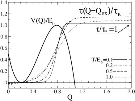
Figure 1: The mean first passage time $\tau(Q=Q_{\text{ex}})\equiv\tau_{\text{mfpt}}(Q_{\text{a}}\to Q_{\text{ex}})$ of (1) (normalized to the $\tau_{\text{K}}$ of (2)) for a cubic potential and different temperatures, defined in units of $E_{\text{b}}$.

As will be demonstrated again below, the $\tau_{\text{mfpt}}(Q_{\text{a}}\to Q_{\text{ex}})$ tends to a constant as soon as the exit point is sufficiently far to the right of the potential barrier. This constant, which henceforth shall simply be called $\tau_{\text{mfpt}}$, becomes identical to the inverse of Kramers’ rate $\tau_{\text{mfpt}}=\tau_{\text{K}}\equiv\hbar/\Gamma_{\text{K}}$, whenever the usual conditions are fulfilled which underly Kramers’ derivation. Recalling that we are dealing with over-damped motion, this $\tau_{\text{K}}$ is given by

$$\tau_{\text{K}}=\frac{2\pi\gamma}{\sqrt{C_{\text{a}}|C_{\text{b}}|}}\exp(E_{\text{b}}/T)\,,$$ (2)

where $C_{\text{a}}$ and $C_{\text{b}}$ are the stiffnesses at the potential minimum and barrier, respectively. In [8] this fact is proven by applying the saddle point approximation to formula (1). For this it is important to have exactly two saddle points, those corresponding to one minimum and one barrier. Notice that the saddle point approximation requires one to replace the barrier by an inverted oscillator, which indeed was also assumed to hold true by Kramers in his famous work.

As a typical case we show in Fig.1 the results of calculations of $\tau_{\text{mfpt}}(Q_{\text{a}}\to Q_{\text{ex}})/\tau_{\text{K}}$ for the same cubic potential as used in [7]. It may be specified by its first derivative to be given by the form

$$V^{\,\prime}(Q)\,\propto\,\left(Q-Q_{\text{a}}\right)\left(Q-Q_{\text{b}}\right)\,,$$ (3)

with the barrier height $E_{\text{b}}=V(Q_{\text{b}})-V(Q_{\text{a}})$ to be $8$ MeV with the extrema to lie at $Q_{\text{a}}\simeq 0.2$ and $Q_{\text{b}}\simeq 0.8$. It is observed that the asymptotic ratio $\tau_{\text{mfpt}}/\tau_{\text{K}}$ becomes close to unity, indeed, if only the parameter temperature over barrier height becomes small enough. However, even for this case of exactly two well pronounced extrema, deviations from unity are clearly visible at larger temperatures.

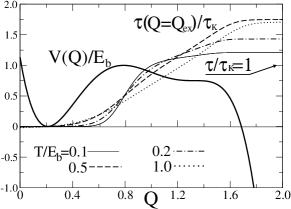
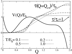
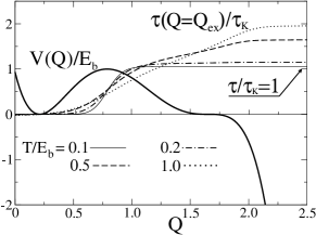
Figure 2: Same as in Fig.1 but for potentials having shoulders at some $Q_{\text{s}}$ of heights $V_{\text{s}}/E_{\text{b}}$ relative to the barrier: $V_{\text{s}}/E_{\text{b}}=0.75$ top left, $0.5$ top right, $0$ bottom left, $-2.5$ bottom right.

This situation becomes more dramatic as soon as the potential shows additional structure. This will now be demonstrated using a schematic potential of fifth order in $Q$. Again, $V(Q)$ will be fixed by its first derivative,

$$V^{\,\prime}(Q)\,\propto\left(Q-Q_{\text{a}}\right)\left(Q-Q_{\text{b}}\right)\left(Q-Q_{\text{c}}\right)\left(Q-Q_{\text{d}}\right)\,,$$ (4)

with $E_{\text{b}}$, $Q_{\text{a}}$ and $Q_{\text{b}}$ unchanged. The remaining two parameters $Q_{\text{c}}$ and $Q_{\text{d}}$ may be used to specify structure of the potential beyond the barrier. In Figs.2 they have been chosen to be identical to one another, $Q_{\text{c}}=Q_{\text{d}}=Q_{\text{s}}$, with their values fixed such that the height $V_{\text{s}}$ of the then existing shoulder takes on the values specified in the figure captions.

In all cases the calculation of $\tau_{\text{mfpt}}(Q_{\text{a}}\to Q_{\text{ex}})$ was performed up to regions of the exit point $Q_{\text{ex}}$ where the stationary value is reached. It is seen that this asymptotic regime is not very far away from the one where the potential is assumed to have additional structure. This is so even for the example shown in the lower right corner of Fig.2. There a potential is taken with a shoulder in a region which lies $20$ MeV below the first minimum, or $-2.5E_{\text{b}}$ in terms of the barrier height. For heavy nuclei this may thus be said to correspond to the scission region after which the fragments separate. The ratio $\tau_{\text{mfpt}}(Q_{\text{a}}\to Q_{\text{ex}})/\tau_{\text{K}}$ shown in the figures is calculated for the $\tau_{\text{K}}$ of (2). Evidently friction drops out but the stiffnesses $C_{\text{a}}$ and $C_{\text{b}}$ from (2) remain. They are taken to be those of the individual potentials for which the $\tau_{\text{mfpt}}$ is computed. These results exhibit clearly the mistake one makes if only Kramers’ rate formula is used to estimate the time the system stays together. Rather, the considerable overshoot of $\tau_{\text{mfpt}}$ over $\tau_{\text{K}}$ indicates that much more time is available for light particles to be emitted before scission. Suppose we look at neutrons. Whenever, their average width $\Gamma_{\text{n}}$ may be used to calculate their multiplicity per fission event from $\Gamma_{\text{n}}/\Gamma_{\text{f}}$ the enhancement of this number over that given by $\Gamma_{\text{n}}/\Gamma_{\text{K}}$ is determined by the ratio $\tau_{\text{mfpt}}/\tau_{\text{K}}$, viz

$$\frac{\Gamma_{\text{n}}}{\Gamma_{\text{f}}}=\frac{\Gamma_{\text{n}}}{\Gamma_{\text{K}}}\frac{\tau_{\text{mfpt}}}{\tau_{\text{K}}}\,.$$ (5)

For the potentials chosen here this enhancement may become quite large.

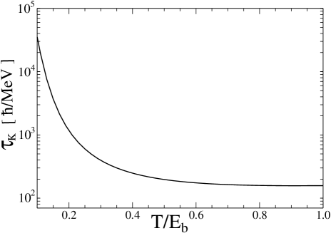
Figure 3: The MFPT corresponding to Kramers’ estimate as function of temperature in units of the barrier height, see text.

To get some feeling for absolute values of this extra available time we estimated the pre-factor $\gamma/\sqrt{C_{\text{a}}|C_{\text{b}}|}$ of (2) following suggestions given in [6]. We simply replaced the geometric mean $\sqrt{C_{\text{a}}|C_{\text{b}}|}$ by the $C$ which there in sect.III.B.5 appears in the relaxation time $\tau_{\text{coll}}$ for over-damped collective motion. Rather than use the formulas given in that section we simply take the results shown in Fig.4 (by the dashed line). Between temperatures of one and four MeV this $\tau_{\text{coll}}$ shows an almost linear dependence in $T$ such that one may write

$$\frac{\gamma}{\sqrt{C_{\text{a}}|C_{\text{b}}|}}=\overline{\tau_{\text{coll}}}\;\simeq\;-\frac{3}{4}+\frac{5}{4}\,T\;\left(\frac{\hbar}{\text{MeV}}\right)\,.$$ (6)

Putting this estimate into the formula given in (2) for $\tau_{\text{K}}(T)$ one obtains the curve shown in Fig.3. The strong temperature dependence reflects the exponential function $\exp(E_{\text{b}}/T)$. As the estimate (6) seizes to be valid above $T\simeq 4$ MeV the curve should not be taken too seriously above $T/E_{\text{b}}\simeq 0.5$. For such a $T$ the $\tau_{\text{K}}$ is about $200\,\hbar/\text{MeV}$ large. As the $\tau_{\text{mfpt}}/\tau_{\text{K}}$ typically is about $1.5$ the additional time increment $\Delta\tau_{\text{f}}=\tau_{\text{mfpt}}-\tau_{\text{K}}$ takes on the sizable value of roughly $100\,\hbar/\text{MeV}$, and, hence, is at least as large as a typical transient time.

Finally, in Fig.4 we look at the case of the potential having a second minimum and maximum. As was to be expected the effect is even larger than before. We would like to remark, however, that this example should be taken with some caution. Commonly, such a double humped barrier comes about because of shell effects. In the range of temperatures considered here the latter may be considered to be quite weak if not already washed out completely. After all our study is concerned with over-damped motion. According to [6] (see also [9]) nuclear collective motion may be expected to become over-damped only above temperatures of about $T=2$ MeV.

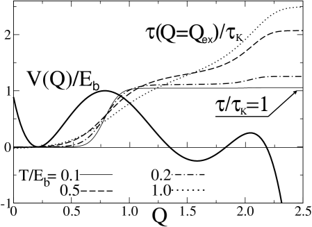
Figure 4: Like in Fig.2 but for a potential having an additional minimum of depth $V_{\text{c}}=-0.25\,E_{\text{b}}$ and a second maximum of height $V_{\text{d}}=0.25\,E_{\text{b}}$.

Our results may be summarized as follows. One of the main issues has been to corroborate features suggested before in [7], and to some extent already in [6]. In essence they imply the following two issues: (i) For situations for which transport equations like those of Kramers or Smoluchowski (or the corresponding Langevin equations) may be applied to analyze fission experiments, it may be inadequate to simply use Kramers’ famous rate formula. Deviations from that may originate in various reasons, for instance in transport coefficients varying with shape, see [6]. Here, we concentrated on properties of the potential restricting ourselves to over-damped motion and the model case of constant friction. (ii) For this model we have been able to demonstrate that there is considerable room for increasing the time the fissioning system stays together without having to rely on concepts which are meaningful only within a time dependent picture. Whereas results obtained within the latter may depend crucially on initial conditions this is not the case for the MFPT [7]. This $\tau_{\text{mfpt}}$ represents the average time it takes for the system to start at the potential minimum and to make its motion all the way out to scission. It includes relaxation processes around the first minimum as well as the sliding down from saddle to scission. The way it is derived [8] implies a proper incorporation of averages over the statistics which are to be associated with a process underlying fluctuating forces. Whereas for Kramers’ model case the $\tau_{\text{mfpt}}$ is nothing else but his inverse rate, this is no longer true for larger temperatures and, in particular, not for potentials of more complicated structure. We have been able to demonstrate that the latter may lead to a considerable prolongation of the time the systems spends before it scissions, allowing in this way for emission of light particles on top of those given by $\Gamma_{\text{n}}/\Gamma_{\text{K}}$. Of course, further work will be necessary to clarify the relevance of this feature with respect to real situations. For such studies not only more realistic potentials have to be used, one should also try to generalize formula (1) to include a coordinate dependent friction coefficient. The ultimate goal should be to be able to use such a formula in a statistical code where one may account for temperatures changing during the process.

Acknowledgements: The authors wish to thank R. Hilton, F.A. Ivanyuk and C. Rummel for useful help. They also wish to acknowledge financial support from the ”Deutsche Forschungsgemeinschaft”. One of us (A.G. Magner) would like to thank the Physik Department of the TUM for the kind hospitality extended to him.

References

- [1] D. Hilscher and H. Rossner, Ann. Phys. Fr. 17 (1992) 471; D. Hilscher, I.I. Gontchar and H. Rossner, Physics of Atomic Nuclei 57 (1994) 1187-1199
- [2] P. Paul and M. Thoennessen, Ann.Rev.Part.Nucl.Sci. 44, (1994) 65.
- [3] H.A. Kramers, Physica 7, 284 (1940).
- [4] D.J. Hofman, B.B. Back, I. Diószegi, C.P. Montoya, S. Schadmand, R.Varma, and P. Paul, Phys. Rev.Let. 72, (1994) 470.
- [5] I. Diószegi, N.P. Shaw, I. Mazumdar, A. Hatzikoutelis and P. Paul, Phys.Rev. C 61, (2000) 024613.
- [6] H. Hofmann, F.A. Ivanyuk, C. Rummel and S. Yamaji, Phys. Rev.C, 64 (2001) 054316
- [7] H. Hofmann and F.A. Ivanyuk, Phys. Rev. Lett.90.132701; see also nucl-th/0302022
- [8] C.W. Gardiner, ”Handbook of stochastic methods, Springer, 2002, Berlin
- [9] H. Hofmann, Phys. Rep. 284 (4&5) (1997)