Hartree-Fock approach to nuclear matter and finite nuclei
with M3Y-type nucleon-nucleon interactions

Abstract

By introducing a density-dependent contact term, M3Y-type interactions applicable to the Hartree-Fock calculations are developed. In order to view basic characters of the interactions, we carry out calculations on the uniform nuclear matter as well as on several doubly magic nuclei. It is shown that a parameter-set called M3Y-P2 describes various properties similarly well to the Skyrme SLy5 and/or the Gogny D1S interactions. A remarkable difference from the SLy5 and the D1S interactions is found in the spin-isospin properties in the nuclear matter, to which the one-pion-exchange potential gives a significant contribution. Affecting the single-particle energies, this difference may play a certain role in the new magic numbers in unstable nuclei.

I Introduction

Various models for nuclear structure have been developed in order to study low energy phenomena of the atomic nuclei. Whereas straightforward application of the bare $NN$ interaction is yet limited only to light nuclei ref:micro , the nuclear structure seems to be well described by relatively simple effective interactions at low energies. Although the effective interactions may depend on the models, there should be basic characters in the effective interactions for the low energy phenomena, irrespective to the models. On the other hand, since the invention of the secondary beam technology, experimental data on the unstable nuclei have disclosed new aspects of the nuclear structure. A remarkable example is the dependence of magic numbers on the neutron excess ref:magic . In regard to the new magic numbers discovered near the neutron drip line, a question has been raised on a character of the effective interactions relating to the spin-isospin flip mode ref:Vst .

Mean-field theories have successfully been applied to the nuclear structure problems, in particular for stable nuclei. They are also useful to investigate basic characters of the effective interactions. However, not many effective interactions have been explored for the nuclear mean-field calculations so far. The Skyrme interaction ref:VB72 has been popular in the Hartree-Fock (HF) calculations, since the zero-range form is easy to be handled. Among a limited number of finite-range interactions, the Gogny interaction ref:Gogny is widely applied to the mean-field calculations, in which the Gaussian form is assumed for the central force. The parameter-sets both of the Skyrme and the Gogny interactions have been adjusted mainly to the data on the nuclei around the $\beta$-stability. It is not obvious whether the available parameter-sets of these interactions account for the new magic numbers properly.

In order to exploit effective interactions applicable also to unstable nuclei, guide from microscopic theories will be important. Brueckner’s $G$-matrix has been a significant clue to studies in this course. Although microscopic approaches using the $G$-matrix have not yet been successful in reproducing the saturation properties, notable progress has been made recently. In the shell model approaches, microscopic effective interactions have been shown to reproduce observed levels remarkably well ref:shell-G . It should be noted, however, that the shell model interactions are usually specific to mass regions, and their global characters have not been discussed in detail, despite several exceptions ref:ST . The so-called Michigan 3-range Yukawa (M3Y) interaction ref:M3Y has been derived from the bare $NN$ interaction, by fitting the Yukawa functions to the $G$-matrix. Represented by the sum of the Yukawa functions, the M3Y-type interactions will be tractable in various models. It has been shown that the M3Y interaction gives matrix elements similar to reliable shell model interactions ref:USD . Moreover, with a certain modification, M3Y-type interactions have successfully been applied to nuclear reactions ref:reac . By using a recently developed algorithm ref:NS02 , a class of the M3Y-type interactions can be applied also to the mean-field calculations. Under such circumstances, it will be of interest to explore M3Y-type interactions and to investigate their characters in the mean-field framework. In this article, we shall develop M3Y-type interactions and investigate their characters via the HF calculations.

II Modification of M3Y interaction

Nuclear effective Hamiltonian consists of the kinetic energy and the effective interaction,

$$H=K+V\,;\quad K=\sum_{i}\frac{\mathbf{p}_{i}^{2}}{2M}\,,\quad V=\sum_{i<j}v_{ij}\,.$$ (1)

Here $i$ and $j$ are the indices of individual nucleons. It will be natural to assume the effective interaction $v_{ij}$ to be translationally invariant, except for the density dependence mentioned below. We consider the effective interaction having the following form,

$$v_{12} = v_{12}^{(\mathrm{C})}+v_{12}^{(\mathrm{LS})}+v_{12}^{(\mathrm{TN})}+v_{12}^{(\mathrm{DD})}\,;$$

$$v_{12}^{(\mathrm{C})} = \sum_{n}(t_{n}^{(\mathrm{SE})}P_{\mathrm{SE}}+t_{n}^{(\mathrm{TE})}P_{\mathrm{TE}}+t_{n}^{(\mathrm{SO})}P_{\mathrm{SO}}+t_{n}^{(\mathrm{TO})}P_{\mathrm{TO}})f_{n}^{(\mathrm{C})}(r_{12})\,,$$

$$v_{12}^{(\mathrm{LS})} = \sum_{n}(t_{n}^{(\mathrm{LSE})}P_{\mathrm{TE}}+t_{n}^{(\mathrm{LSO})}P_{\mathrm{TO}})f_{n}^{(\mathrm{LS})}(r_{12})\,\mathbf{L}_{12}\cdot(\mathbf{s}_{1}+\mathbf{s}_{2})\,,$$

$$v_{12}^{(\mathrm{TN})} = \sum_{n}(t_{n}^{(\mathrm{TNE})}P_{\mathrm{TE}}+t_{n}^{(\mathrm{TNO})}P_{\mathrm{TO}})f_{n}^{(\mathrm{TN})}(r_{12})\,r_{12}^{2}S_{12}\,,$$

$$v_{12}^{(\mathrm{DD})} = t^{(\mathrm{DD})}(1+x^{(\mathrm{DD})}P_{\sigma})[\rho(\mathbf{r}_{1})]^{\alpha}\delta(\mathbf{r}_{12})\,.$$ (2)

The relative coordinate is denoted by $\mathbf{r}_{12}=\mathbf{r}_{1}-\mathbf{r}_{2}$ and $r_{12}=|\mathbf{r}_{12}|$. Correspondingly, the relative momentum is defined by $\mathbf{p}_{12}=(\mathbf{p}_{1}-\mathbf{p}_{2})/2$. $\mathbf{L}_{12}$ is the relative orbital angular momentum,

$$\mathbf{L}_{12}=\mathbf{r}_{12}\times\mathbf{p}_{12}\,,$$ (3)

$\mathbf{s}_{1}$, $\mathbf{s}_{2}$ are the nucleon spin operators, and $S_{12}$ is the tensor operator,

$$S_{12}=4\,[3(\mathbf{s}_{1}\cdot\hat{\mathbf{r}}_{12})(\mathbf{s}_{2}\cdot\hat{\mathbf{r}}_{12})-\mathbf{s}_{1}\cdot\mathbf{s}_{2}]\,.$$ (4)

$f_{n}(r_{12})$ represents an appropriate function of $r_{12}$, the subscript $n$ corresponds to the parameter attached to the function (e.g. the range of the interaction), and $t_{n}$ is the coefficient. Examples of $f_{n}(r_{12})$ are the delta, the Gauss and the Yukawa functions. $P_{\sigma}$ ($P_{\tau}$) denotes the spin (isospin) exchange operator, while $P_{\mathrm{SE}}$, $P_{\mathrm{TE}}$, $P_{\mathrm{SO}}$ and $P_{\mathrm{TO}}$ are the projection operators on the singlet-even (SE), triplet-even (TE), singlet-odd (SO) and triplet-odd (TO) two-particle states, respectively, which are defined by

$$P_{\mathrm{SE}}=\frac{1-P_{\sigma}}{2}\,\frac{1+P_{\tau}}{2}\,,\quad P_{\mathrm{TE}}=\frac{1+P_{\sigma}}{2}\,\frac{1-P_{\tau}}{2}\,,$$

$$P_{\mathrm{SO}}=\frac{1-P_{\sigma}}{2}\,\frac{1-P_{\tau}}{2}\,.\quad P_{\mathrm{TO}}=\frac{1+P_{\sigma}}{2}\,\frac{1+P_{\tau}}{2}\,.$$ (5)

The nucleon density is denoted by $\rho(\mathbf{r})$. The original M3Y interaction is represented in the form of Eq. (2), with $f_{n}(r_{12})=e^{-\mu_{n}r_{12}}/\mu_{n}r_{12}$ and $v_{12}^{(\mathrm{DD})}=0$. As discussed in Ref. ref:NS02 , the Skyrme and the Gogny interactions are obtained by setting $f_{n}(r_{12})$ appropriately, except for some parameter-sets of the Skyrme interaction in which certain terms are expressed only in the density-functional form.

The saturation of density and energy is a basic property of nuclei. In developing effective interactions adaptable for many nuclei, it is required to reproduce the saturation property. However, the non-relativistic $G$-matrix fails to reproduce the saturation at the right density and energy. Therefore, it will not be appropriate to use the $G$-matrix for HF calculations without any modification, although several HF approaches using interactions derived from the $G$-matrix were tried in earlier studies ref:Neg70 . The M3Y interaction was obtained so that the $G$-matrix at a certain density could be reproduced by a sum of the Yukawa functions. The M3Y interaction gives no saturation point within the HF theory, unless density-dependence is taken into account explicitly. Khoa et al. applied the M3Y interaction to nuclear reactions in the folding model, by making the coupling constants dependent on densities ref:reac . In their approach the exchange terms are treated approximately. However, the exchange terms may contribute quite significantly to the nuclear structure. We here keep the coupling constants in $v_{12}^{(\mathrm{C})}$ independent of density, while introduce a density-dependent contact interaction ($v_{12}^{(\mathrm{DD})}$ in Eq. (2)), as in the Skyrme and the Gogny interactions. We can then treat the exchange (i.e. the Fock) terms exactly with the currently available computers. It should be mentioned that there has been an interesting attempt to approximate the exchange terms of the interaction in the density-matrix expansion ref:HL98 , although the accuracy of the density-matrix expansion should be checked carefully.

We start from the Paris-potential version of the M3Y interaction ref:M3Y-P . This original parameter-set with no density-dependence is hereafter called ‘M3Y-P0’. We shall modify this interaction so as to reproduce the saturation properties. In the isotropic uniform nuclear matter, matrix elements of $v_{12}^{(\mathrm{LS})}$ and $v_{12}^{(\mathrm{TN})}$ between the HF states vanish. Therefore $v_{12}^{(\mathrm{C})}+v_{12}^{(\mathrm{DD})}$ determines the bulk properties such as the saturation. The range parameters for the Yukawa functions $f^{(\mathrm{C})}_{n}(r_{12})=e^{-\mu_{n}r_{12}}/\mu_{n}r_{12}$ in $v_{12}^{(\mathrm{C})}$ are $\mu_{1}^{-1}=0.25$, $\mu_{2}^{-1}=0.4$ and $\mu_{3}^{-1}=1.414\,\mathrm{fm}$ in the M3Y interaction, which correspond to the Compton wave-lengths of mesons with masses of about 790, 490 and 140 MeV, respectively. We do not change these parameters. For the longest-range part ($n=3$), the coupling constants $t_{3}^{(\mathrm{SE})}$, $t_{3}^{(\mathrm{TE})}$, $t_{3}^{(\mathrm{SO})}$ and $t_{3}^{(\mathrm{TO})}$ are fixed to be those of the one-pion-exchange potential (OPEP), as in M3Y-P0. The interaction $v_{12}^{(\mathrm{DD})}$ in Eq. (2) acts only on the SE and TE channels,

$$v_{12}^{(\mathrm{DD})}=t^{(\mathrm{DD})}(1-x^{(\mathrm{DD})})\delta(\mathbf{r}_{12})P_{\mathrm{SE}}+t^{(\mathrm{DD})}(1+x^{(\mathrm{DD})})\delta(\mathbf{r}_{12})P_{\mathrm{TE}}\,.$$ (6)

Microscopic investigations have shown that the density-dependence of the TE part is primarily responsible for the saturation ref:Bet71 , as a higher-order effect of the tensor force. While the interaction in the SE channel is attractive at low densities, it also has certain density-dependence originating in the strong short-range repulsion. Thus, a possible way of modifying the M3Y interaction may be to replace a fraction of the repulsion in the SE and TE channels by $v_{12}^{(\mathrm{DD})}$.

In addition to the saturation properties which are relevant to the central force, the LS splitting is significant in describing the shell structure of nuclei. While true origin of the LS splitting is not yet obvious ref:LS , LS splittings obtained from HF calculations with the $G$-matrix interaction are too small, in comparison with the observed ones. From the HF calculations for finite nuclei, we find that $v_{12}^{(\mathrm{LS})}$ should be about twice as strong as that of M3Y-P0 to reproduce the observed LS splittings. The tensor force influences the ordering of the single-particle (s.p.) orbits. To reproduce the observed ordering, $v_{12}^{(\mathrm{TN})}$ should be smaller than that of M3Y-P0. We here introduce an overall enhancement factor to $v_{12}^{\mathrm{(LS)}}$ and an overall reduction factor to $v_{12}^{\mathrm{(TN)}}$, as will be shown in Section V.

In this paper we shall use two parameter-sets for modified M3Y interaction, ‘M3Y-P1’ and ‘M3Y-P2’, in order to show sensitivity to the parameters for some results. In M3Y-P1, we replace the shortest-range ($n=1$) repulsive part of $v_{12}^{\mathrm{(C)}}$ by $v_{12}^{(\mathrm{DD})}$ in a simple manner. We reduce both $t_{1}^{(\mathrm{SE})}$ and $t_{1}^{(\mathrm{TE})}$ by a single factor, keeping the SE/TE ratio in $v_{12}^{(\mathrm{DD})}$ to be equal to $t_{1}^{(\mathrm{SE})}/t_{1}^{(\mathrm{TE})}$ in M3Y-P0, by imposing

$$x^{(\mathrm{DD})}=\frac{t_{1}^{(\mathrm{TE})}-t_{1}^{(\mathrm{SE})}}{t_{1}^{(\mathrm{TE})}+t_{1}^{(\mathrm{SE})}}\,.$$ (7)

The reduction factor and $t^{(\mathrm{DD})}$ are determined so as for the saturation density and energy in the nuclear matter to be typical values, as presented in the subsequent section. Characters of M3Y-P1 will be investigated in the nuclear matter. Although this modification is too simple to reproduce properties of finite nuclei, the M3Y-P1 set will be useful to clarify what characters arise from the original M3Y interaction, relatively insensitive to the phenomenological modification. In the M3Y-P2 set, all $t_{n}$ parameters belonging to the $n=1$ and $2$ channels in $v_{12}^{(\mathrm{C})}$ are shifted from those of M3Y-P0. Although we have three ranges in $v_{12}^{(\mathrm{C})}$, the number of adjustable parameters is no greater than in the Gogny interaction, since we fix the OPEP part. We fit those parameters, together with the enhancement factor for $v_{12}^{(\mathrm{LS})}$ and the reduction factor for $v_{12}^{(\mathrm{TN})}$, to the binding energies of several doubly magic nuclei. The resultant values of the parameters will be shown later.

III Properties of nuclear matter at and around saturation point

Basic characters of nuclear effective interactions can be discussed via properties of the infinite nuclear matter; in particular, properties at and around the saturation point. In this section we investigate characters of the M3Y-type interactions via the nuclear matter properties within the HF theory. In comparison, we also discuss those of the Skyrme and the Gogny interactions. We use the D1S parameter-set ref:D1S for the Gogny interaction. In most of the Skyrme HF approaches, the LS currents arising from the momentum-dependence of the central force are ignored, and the parameters are adjusted without their contribution. Although this treatment occasionally improves some characters of the interactions, in this paper we would focus on characters of the two-body interactions, rather than those of density functionals. For this reason we adopt the SLy5 set ref:SLy , which is devised for calculations including the LS currents.

In the HF theory of the nuclear matter, the s.p. wave-functions can be taken to be the plane wave,

$$\varphi_{\mathbf{k}\sigma\tau}(\mathbf{r})=\frac{1}{\sqrt{\Omega}}\,e^{i\mathbf{k}\cdot\mathbf{r}}\,\chi_{\sigma}\chi_{\tau}\,.$$ (8)

Here $\chi_{\sigma}$ ($\chi_{\tau}$) denotes the spin (isospin) wave-function, and $\Omega$ indicates the volume of the system, for which we will take the $\Omega\rightarrow\infty$ limit afterward. The s.p. energy for this state is defined as

$$\epsilon(\mathbf{k}\sigma\tau)=\frac{\mathbf{k}^{2}}{2M}+\frac{\Omega}{(2\pi)^{3}}\sum_{\sigma_{2}\tau_{2}}\int_{k_{2}\leq k_{\mathrm{F}\tau_{2}\sigma_{2}}}d^{3}k_{2}\langle\mathbf{k}\sigma\tau,\mathbf{k}_{2}\sigma_{2}\tau_{2}|v_{12}|\mathbf{k}\sigma\tau,\mathbf{k}_{2}\sigma_{2}\tau_{2}\rangle\,.$$ (9)

Energy of the nuclear matter is expressed by a function of densities depending on the spin and the isospin, $\rho_{\tau\sigma}$ ($\tau=p,n$; $\sigma=\uparrow,\downarrow$). The density variables can be converted to the total density $\rho={\displaystyle\sum_{\sigma\tau}}\rho_{\tau\sigma}$, and the spin- and isospin-asymmetry parameters

$$\eta_{s} = \frac{{\displaystyle\sum_{\sigma\tau}}\sigma\rho_{\tau\sigma}}{\rho}~{}=~{}\frac{\rho_{p\uparrow}-\rho_{p\downarrow}+\rho_{n\uparrow}-\rho_{n\downarrow}}{\rho}\,,$$

$$\eta_{t} = \frac{{\displaystyle\sum_{\sigma\tau}}\tau\rho_{\tau\sigma}}{\rho}~{}=~{}\frac{\rho_{p\uparrow}+\rho_{p\downarrow}-\rho_{n\uparrow}-\rho_{n\downarrow}}{\rho}\,,$$

$$\eta_{st} = \frac{{\displaystyle\sum_{\sigma\tau}}\sigma\tau\rho_{\tau\sigma}}{\rho}~{}=~{}\frac{\rho_{p\uparrow}-\rho_{p\downarrow}-\rho_{n\uparrow}+\rho_{n\downarrow}}{\rho}\,,$$ (10)

where $\sigma$ ($\tau$) in the summation takes $\pm 1$, corresponding to $\sigma=\uparrow,\downarrow$ ($\tau=p,n$). By assuming that the s.p. states are occupied up to the Fermi momentum, the density is related to the Fermi momentum for each spin and isospin,

$$\rho_{\tau\sigma}=\frac{1}{6\pi^{2}}k_{\mathrm{F}\tau\sigma}^{3}\,.$$ (11)

The total energy of nuclear matter is given by

$$E = \frac{\Omega}{(2\pi)^{3}}\sum_{\sigma_{1}\tau_{1}}\int_{k_{1}\leq k_{\mathrm{F}\tau_{1}\sigma_{1}}}d^{3}k_{1}\frac{\mathbf{k}_{1}^{2}}{2M}$$

$$+\frac{\Omega^{2}}{2(2\pi)^{6}}\sum_{\sigma_{1}\sigma_{2}\tau_{1}\tau_{2}}\int_{k_{1}\leq k_{\mathrm{F}\tau_{1}\sigma_{1}}}d^{3}k_{1}\int_{k_{2}\leq k_{\mathrm{F}\tau_{2}\sigma_{2}}}d^{3}k_{2}\langle\mathbf{k}_{1}\sigma_{1}\tau_{1},\mathbf{k}_{2}\sigma_{2}\tau_{2}|v_{12}|\mathbf{k}_{1}\sigma_{1}\tau_{1},\mathbf{k}_{2}\sigma_{2}\tau_{2}\rangle\,.$$

As already pointed out, only $v_{12}^{(\mathrm{C})}+v_{12}^{(\mathrm{DD})}$ contributes to the energy of the isotropic nuclear matter. In Appendix A, several formulae on the HF energy of the nuclear matter are derived for interactions expressed in the form of Eq. (2), with general and typical $f^{(\mathrm{C})}_{n}(r_{12})$. As well as for the M3Y-type interactions, the nuclear matter energies are calculated for the Skyrme and the Gogny interactions by using these formulae.

In the spin-saturated symmetric nuclear matter, we have $\eta_{s}=\eta_{t}=\eta_{st}=0$, which indicates $k_{\mathrm{F}p\uparrow}=k_{\mathrm{F}p\downarrow}=k_{\mathrm{F}n\uparrow}=k_{\mathrm{F}n\downarrow}$ and $\rho_{p\uparrow}=\rho_{p\downarrow}=\rho_{n\uparrow}=\rho_{n\downarrow}=\rho/4$. In this case we denote the Fermi momentum simply by $k_{\mathrm{F}}$. The lowest energy for a given $\rho$ normally occurs along this line. The saturation point is obtained by minimizing the energy per nucleon $\mathcal{E}=E/A$,

$$\left.\frac{\partial\mathcal{E}}{\partial\rho}\right|_{\mathrm{sat.}}=0\,,$$ (13)

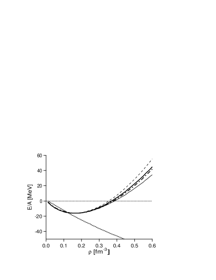
Figure 1: Energies per nucleon $\mathcal{E}=E/A$ in the symmetric nuclear matter for several effective interactions. The thick dotted, dot-dashed and solid lines represent the results with the M3Y-P0, M3Y-P1 and M3Y-P2 interactions, respectively, while the thin dashed and solid lines those with the SLy5 and D1S interactions.

which yields the saturation density $\rho_{0}$ (equivalently, $k_{\mathrm{F}0}$) and energy $\mathcal{E}_{0}$. Figure 1 illustrates $\mathcal{E}$ as a function of $\rho$ for the symmetric nuclear matter with the M3Y-type as well as with the SLy5 and D1S effective interactions. We set $M=(M_{p}+M_{n})/2$, where $M_{p}$ ($M_{n}$) is the measured mass of a proton (a neutron). The parameters for $v_{12}^{(\mathrm{C})}$ and $v_{12}^{(\mathrm{DD})}$ of the M3Y-type interactions are listed in Table 1. As mentioned above, the M3Y-P0 interaction gives no saturation point. We do have saturation points in M3Y-P1 and M3Y-P2 owing to $v_{12}^{(\mathrm{DD})}$. Differences among the saturating forces, i.e. SLy5, D1S, M3Y-P1 and M3Y-P2, are small at $\rho\lesssim\rho_{0}$. At relatively high density ($\rho\gtrsim 0.3\,\mathrm{fm}^{-3}$), the M3Y-P1 and the M3Y-P2 interactions have lower $\mathcal{E}$ than SLy5 and higher than D1S. The values of $k_{\mathrm{F}0}$ and $\mathcal{E}_{0}$ are tabulated in Table 2. The M3Y-P1 set has been determined so as to give $k_{\mathrm{F}0}\simeq 1.36\,\mathrm{fm}$ and $\mathcal{E}_{0}\simeq 16\,\mathrm{MeV}$.

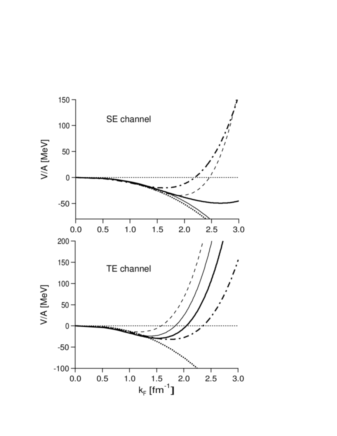
Figure 2: Contribution of the SE and TE channels to $\mathcal{E}$. See Fig. 1 for conventions.

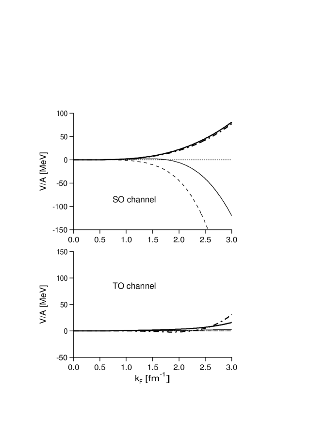
Figure 3: Contribution of the SO and TO channels to $\mathcal{E}$. In both channels, the results of M3Y-P0 is equal to those of M3Y-P1, which are presented by the dot-dashed line. See Fig. 1 for the other conventions.

In Figs. 2 and 3, contribution to $\mathcal{E}$ from each of the SE, TE, SO and TO channels in $v_{12}^{(\mathrm{C})}+v_{12}^{(\mathrm{DD})}$ is shown as a function of $k_{\mathrm{F}}$. Sum of all these channels and the kinetic energy $\langle K\rangle/A=(3/5)(k_{\mathrm{F}}^{2}/2M)$ is equal to $\mathcal{E}$ in Fig. 1. As is viewed in Fig. 2, the TE channel takes a minimum at $k_{\mathrm{F}}=1.3-1.5\,\mathrm{fm}$ except for M3Y-P0 and M3Y-P1, primarily responsible for the saturation at $k_{\mathrm{F}0}\approx 1.3\,\mathrm{fm}$. In the D1S interaction, the energy out of the SE channel monotonically goes down. This is not compatible with the presence of the strong short-range repulsion in the $NN$ force, and causes an unphysical property in the neutron matter, as will be shown in Section IV. Both the SO and TO channels do not contribute to $\mathcal{E}$ significantly for $\rho\lesssim\rho_{0}$ (i.e. $k_{\mathrm{F}}\lesssim k_{\mathrm{F}0}$). While the SO channel becomes attractive and the TO channel stays small in the SLy5 and the D1S interactions, both channels are repulsive in the M3Y-type interactions at $\rho>\rho_{0}$, including M3Y-P0. A certain part of this character of the M3Y-type interactions comes from the OPEP part.

The curvature at the saturation point with respect to $\rho$ is proportional to the incompressibility,

$$\mathcal{K}=k_{\mathrm{F}}^{2}\left.\frac{\partial^{2}\mathcal{E}}{\partial k_{\mathrm{F}}^{2}}\right|_{\mathrm{sat.}}=9\rho^{2}\left.\frac{\partial^{2}\mathcal{E}}{\partial\rho^{2}}\right|_{\mathrm{sat.}}\,.$$ (14)

The effective mass ($k$-mass) at the saturation point $M^{\ast}_{0}$ is defined by

$$\left.\frac{\partial\epsilon(\mathbf{k}\sigma\tau)}{\partial k}\right|_{\mathrm{sat.}}=\frac{k_{\mathrm{F}0}}{M^{\ast}_{0}}\,.$$ (15)

The volume asymmetry energy corresponds to the curvature of $\mathcal{E}$ with respect to $\eta_{t}$,

$$a_{t}=\left.\frac{1}{2}\frac{\partial^{2}\mathcal{E}}{\partial\eta_{t}^{2}}\right|_{\mathrm{sat.}}\,.$$ (16)

Analogously, the following coefficients are defined from the curvatures of $\mathcal{E}$ with respect to $\eta_{s}$ and $\eta_{st}$,

$$a_{s}=\left.\frac{1}{2}\frac{\partial^{2}\mathcal{E}}{\partial\eta_{s}^{2}}\right|_{\mathrm{sat.}}\,,\quad\quad a_{st}=\left.\frac{1}{2}\frac{\partial^{2}\mathcal{E}}{\partial\eta_{st}^{2}}\right|_{\mathrm{sat.}}\,.$$ (17)

These coefficients $a_{s}$, $a_{t}$ and $a_{st}$ are relevant to the spin and isospin responses in finite nuclei. In Table 2 we also compare $\mathcal{K}$, $M_{0}^{\ast}$, $a_{t}$, $a_{s}$ and $a_{st}$ among the effective interactions.

The incompressibility $\mathcal{K}$ is sensitive to $\alpha$ in $v_{12}^{(\mathrm{DD})}$. The experimental value of $\mathcal{K}$ has been extracted from the excitation energies of the giant monopole resonances. Despite a certain model-dependence, most non-relativistic models are consistent with the experiments if $\mathcal{K}\approx 210\,\mathrm{MeV}$. For finite-range interactions, i.e. the Gogny and the M3Y-type interactions, $\alpha\approx 1/3$ seems to give reasonable values of $\mathcal{K}$, while in the Skyrme interactions $\alpha\approx 1/6$ looks favorable, because of the momentum-dependent terms in $v_{12}^{(\mathrm{C})}$. The $k$-mass is empirically known to be $M_{0}^{\ast}\approx(0.6-0.7)M$ ref:Mahaux . The M3Y-type interactions tend to yield slightly smaller $M_{0}^{\ast}$ than the SLy5 and the D1S interactions. The volume asymmetry energy $a_{t}$ is important in reproducing global trend of the binding energies for the $Z\neq N$ nuclei. From empirical viewpoints $a_{t}\approx 30\,\mathrm{MeV}$ seems appropriate, as is fulfilled in the M3Y-type interactions under consideration.

The $a_{s}$ and $a_{st}$ coefficients are relevant to the spin degrees of freedom. The kinetic energy has a certain contribution to $a_{s}$ and $a_{st}$, as well as to $a_{t}$, which amounts to about $12\,\mathrm{MeV}$ at $\rho\approx\rho_{0}$ equally for $a_{t}$, $a_{s}$ and $a_{st}$. The interaction $v_{12}^{(\mathrm{C})}+v_{12}^{(\mathrm{DD})}$ gives rise to the rest of these coefficients. Both the M3Y-type interactions have similar tendency with respect to these coefficients. It is remarkable that $a_{st}$ is substantially larger in the M3Y-type interactions than $a_{s}$. As is suggested by close $a_{s}$ and $a_{st}$ values between M3Y-P1 and M3Y-P2, the original M3Y interaction already carries this feature. In particular, the OPEP part included in the M3Y-type interactions plays a significant role, increasing $a_{st}$ by about $11\,\mathrm{MeV}$. On the other hand, $a_{s}$ and $a_{st}$ are comparable in the Gogny D1S interaction, and we have even $a_{s}>a_{st}$ in the Skyrme SLy5 interaction. In the SLy5 case, $a_{st}$ is close to the value due only to the kinetic energy.

Global characters of the spin and isospin responses are customarily discussed in terms of the Landau parameters. Formulae on the Landau parameters at the zero temperature are given in Appendix B. We compute the parameters of Eq. (73). The results are shown in Table 3. It is remarked that the M3Y-P1 and M3Y-P2 interactions give similar results. The $g_{\ell}$ and the $g^{\prime}_{\ell}$ parameters are closely related to the $a_{s}$ and the $a_{st}$ coefficients, respectively. It has been known that $g_{0}$ is small, while $g^{\prime}_{0}$ should be relatively large ref:g'0 . Although it is not easy to extract precise values of the Landau parameters from experimental data because they could depend on the interaction forms, qualitative trend will not depend on effective interactions. The M3Y-type interactions seem to have reasonable characters on the spin and isospin responses, while SLy5 and D1S do not, although the spin and isospin natures of the Skyrme interactions seem to be improved if the LS currents are ignored ref:Lan-Sky . It is likely that the difference in these coefficients may significantly influence predictions of the spin and isospin responses of finite nuclei.

IV Properties of asymmetric nuclear matter and neutron matter

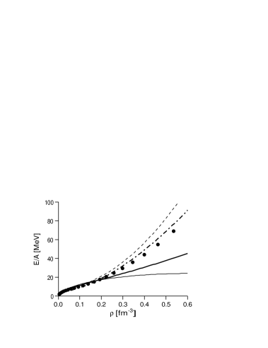
Figure 5: Energies per nucleon $\mathcal{E}=E/A$ in the neutron matter for several effective interactions. The circles are the results of Ref. ref:FP81 . See Fig. 1 for the other conventions.

We turn to the asymmetric nuclear matter. In Fig. 4, energies per nucleon $\mathcal{E}$ are depicted as a functions of $\rho$ for the spin-saturated (i.e. $\eta_{s}=\eta_{st}=0$) nuclear matter with $\eta_{t}=-0.2$ and $-0.5$. The results from the M3Y-type interactions are compared with those of the Skyrme and the Gogny interactions. Energies of the spin-saturated neutron matter (i.e. $\eta_{t}=-1$) are presented in Fig. 5. Results from a microscopic calculation in Ref. ref:FP81 are also shown as a reference. Although the dependence on the interactions is not strong at low densities even for the neutron matter, it becomes stronger at $\rho>0.2\,\mathrm{fm}$ as $|\eta_{t}|$ increases. In the D1S result for the neutron matter, $\mathcal{E}$ has a maximum at $\rho\approx 0.6\,\mathrm{fm}$ and goes to $-\infty$ as $\rho\rightarrow\infty$. This unphysical behavior arises from $x^{(\mathrm{DD})}=1$ in the D1S set, which implies no density-dependence in the SE channel (see Eq. (6)). This could also give rise to a problem in practical calculations for finite nuclei. With the SLy5 interaction $\mathcal{E}$ goes up rapidly at any $\eta_{t}$, because of the momentum-dependence of the interaction. In contrast to them, the M3Y-type interactions give moderate $\mathcal{E}$ for the neutron matter. The microscopic energy of Ref. ref:FP81 lies between those of M3Y-P1 and M3Y-P2. It will be possible, if necessary, to adjust the parameters of the M3Y-type interactions to the microscopic results.

V Properties of doubly magic nuclei

We next discuss properties of doubly magic nuclei in the HF approximation. In the calculations for finite nuclei, we use the algorithm presented in Ref. ref:NS02 , where the following s.p. bases are employed,

$$\varphi_{\alpha\ell jm}(\mathbf{r}) = R_{\alpha\ell j}(r)[Y^{(\ell)}(\hat{\mathbf{r}})\chi_{\sigma}]^{(j)}_{m}\,;$$

$$R_{\alpha\ell j}(r) = \mathcal{N}_{\alpha\ell j}\,r^{\ell+2p_{\alpha}}\exp[-(r/\nu_{\alpha})^{2}]\,.$$ (18)

Here $Y^{(\ell)}(\hat{\mathbf{r}})$ expresses the spherical harmonics. We drop the isospin index without confusion. The index $\alpha$ indicates $p_{\alpha}$ (a non-negative integer) and $\nu_{\alpha}$, simultaneously. By choosing $p_{\alpha}$ and $\nu_{\alpha}$ appropriately, these bases span the space equivalent to that of the harmonic-oscillator (HO) bases, as well as they can form the Kamimura-Gauss (KG) basis-set ref:KKF . Without parameters specific to mass number or nuclide such as $\hbar\omega$, a single set of the KG bases is applicable to wide range of nuclides. In the following calculations we apply the hybrid basis-set ref:NS02 for the nuclei with $A<50$, in which an HO basis is added to the KG basis-set, while the HO basis-set with $N_{\mathrm{osc}}\leq 15$ and $\hbar\omega=41.2A^{-1/3}\,\mathrm{MeV}$ for heavier nuclei.

In finite nuclei the non-central forces are important as well. In the M3Y interaction, the LS force $v_{12}^{(\mathrm{LS})}$ and the tensor force $v_{12}^{(\mathrm{TN})}$ are taken by setting $f_{n}^{(\mathrm{LS})}(r_{12})=e^{-\mu_{n}r_{12}}/\mu_{n}r_{12}$ and $f_{n}^{(\mathrm{TN})}(r_{12})=e^{-\mu_{n}r_{12}}/\mu_{n}r_{12}$ in Eq. (2). We here fix the range parameters as in $v_{12}^{(\mathrm{C})}$; $\mu_{1}^{-1}=0.25\,\textrm{fm}$, $\mu_{2}^{-1}=0.4\,\textrm{fm}$ for $v_{12}^{(\mathrm{LS})}$, and $\mu_{1}^{-1}=0.4\,\textrm{fm}$, $\mu_{2}^{-1}=0.7\,\textrm{fm}$ for $v_{12}^{(\mathrm{TN})}$. The coupling constants in the M3Y-P2 set are tabulated in Table 4, together with those in the original M3Y-P0 set. In M3Y-P2, the enhancement factor for $v_{12}^{(\mathrm{LS})}$ is taken to be 1.8 and the reduction factor for $v_{12}^{(\mathrm{TN})}$ to be 0.12. The binding energies and the rms matter radii obtained from the HF calculations with M3Y-P2 are shown in Table 5, in comparison with those of the SLy5 and the D1S interactions, as well as with the experimental data. The one-body terms of the center-of-mass (c.m.) energy are removed before iteration. The contribution of the two-body terms is subtracted from the convergent HF wave-functions, in the D1S and the M3Y-P2 results. There are also spurious c.m. effects in the matter radii,

$$\langle r^{2}\rangle = \frac{1}{A}\sum_{i}\langle(\mathbf{r}_{i}-\mathbf{R})^{2}\rangle~{}=~{}\frac{1}{A}\sum_{i}\langle r_{i}^{2}\rangle-\langle R^{2}\rangle$$ (19)

$$= \frac{1}{A}\left[\left(1-\frac{1}{A}\right)\sum_{i}\langle r_{i}^{2}\rangle-\frac{1}{A}\sum_{i\neq j}\langle\mathbf{r}_{i}\cdot\mathbf{r}_{j}\rangle\right]\,.$$

The first term in the right-hand side is expressed by one-body operators with a correction factor $(1-1/A)$. We need two-body operators for the second term. For the D1S and the M3Y-P2 interactions we fully remove the c.m. contribution according to Eq. (19). For the SLy5 interaction we use only the one-body terms with the correction factor, ignoring the two-body terms in Eq. (19), as in calculating the energies.

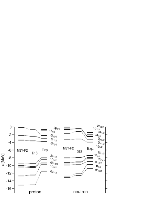
Figure 6: Single-particle energies for ²⁰⁸Pb. Experimental values are extracted from Refs. ref:mass ; ref:TI .

Wave-functions of the doubly magic nuclei are considered to be well approximated in the spherical HF approaches. It should still be noted that correlations due to the residual interaction could influence their properties. Therefore we do not pursue fine tuning of the parameters. As shown in Table 5, the M3Y-P2 set is fixed so as to reproduce the measured binding energies of the doubly magic nuclei, including ⁹⁰Zr, within about 5 MeV accuracy. The binding energies of these nuclei obtained from the SLy5 and the D1S interactions are in agreement with the experimental data within 3 MeV, slightly better than M3Y-P2. We do not have to take this difference seriously, before evaluating influence of the residual interactions. As well as the binding energies, the rms matter radii of these nuclei are reproduced by the M3Y-P2 set similarly well to the other available interactions. In Table 6 we present the neutron s.p. energies $\epsilon_{n}(0p_{3/2})$ and $\epsilon_{n}(0p_{1/2})$ around ¹⁶O. The enhancement factor for $v_{12}^{(\mathrm{LS})}$ in the M3Y-P2 set has been adjusted approximately to the experimental value of this s.p. energy difference. The reduction factor for $v_{12}^{(\mathrm{TN})}$ has been determined so as to reproduce the s.p. energy ordering for ²⁰⁸Pb. Without this reduction factor, the orbits with higher $\ell$ have too high energies. The resultant s.p. levels in ²⁰⁸Pb with M3Y-P2 are depicted in Fig. 6. The levels obtained from D1S and the experimental s.p. levels are also shown. The overall level spacings are related to $M^{\ast}_{0}$ shown in Table 2. In the usual HF calculations the level spacings tend to be larger than the observed ones, and it is not (and should not be) remedied until the correlations due to the residual interaction (or the $\omega$-mass) are taken into account ref:Mahaux . This is also true in the present case. We find that M3Y-P2 yields as plausible s.p. levels as D1S does. We thus confirm that the M3Y-P2 interaction well describes global nature of stable nuclei.

VI Single particle levels in $N=16$ isotones

In the preceding section we have shown that the M3Y-P2 interaction reproduces the properties of the doubly magic nuclei to a similar accuracy to the SLy5 and the D1S interactions. At a glance, the spin-isospin characters in the nuclear matter, which have been discussed in Section III via $a_{st}$ and $g^{\prime}_{\ell}$, do not seem to influence the nuclear properties around the ground states. However, the spin and isospin characters influence s.p. energies of finite nuclei. Thereby they may affect even the ground state properties. In this section we illustrate this point by the neutron orbits in the $N=16$ isotones, following the arguments in Ref. ref:Vst , although precise studies in this line are beyond scope of this paper.

As was suggested in Ref. ref:Vst , the proton-number ($Z$) dependence of the neutron s.p. energy $\epsilon_{n}(0d_{3/2})$ relative to $\epsilon_{n}(1s_{1/2})$ can sizably be affected by effective interactions. Figure 7 depicts ${\mathit{\Delta}}\epsilon_{n}=\epsilon_{n}(0d_{3/2})-\epsilon_{n}(1s_{1/2})$ obtained from the spherical HF calculations in the $N=16$ isotones. Though it is not obvious whether the ground states of all of these isotones are well approximated by the spherical HF wave-functions, it is meaningful to see the s.p. energies, which often give an indication to magic or submagic numbers. For D1S we reduce the number of bases in Eq. (18) to avoid instability occurring for some $N=16$ nuclei, which probably relates to the unphysical behavior in the neutron matter. It is found that, if viewed as a function of $Z$, ${\mathit{\Delta}}\epsilon_{n}$ strikingly depends on the interactions. With the M3Y-P2 interaction, ${\mathit{\Delta}}\epsilon_{n}$ increases as $Z$ goes from $Z=14$ to $Z=8$. We have confirmed ref:Nak02 that even M3Y-P1 (with appropriate $v_{12}^{(\mathrm{LS})}$ and $v_{12}^{(\mathrm{TN})}$) shows similar behavior and that a significant part of this feature originates in the OPEP part in $v_{12}^{(\mathrm{C})}$. It is thus suggested that this behavior of ${\mathit{\Delta}}\epsilon_{n}$ is correlated to the spin-isospin property in the nuclear matter.

For comparison, we also show the s.p. energies obtained from the reliable shell model interaction for the $sd$-shell nuclei, the so-called USD interaction ref:USD . For this purpose we define effective values of the s.p. energies for each nucleus $A$ from the shell model space and interaction, which correspond to those of the spherical HF calculations, as

$$\epsilon_{n}^{\mathrm{USD}}(j;A)=\epsilon_{n}^{\mathrm{USD}}(j;^{\,17\!}\mathrm{O})+\sum_{j^{\prime}}\langle N_{j^{\prime}}\rangle_{A}\,\frac{2J+1}{(2j+1)(2j^{\prime}+1)}\,\langle jj^{\prime};J|v^{\mathrm{USD}}|jj^{\prime};J\rangle\,,$$ (20)

where the sum with respect to $j^{\prime}$ runs over the valence orbits. For $\langle N_{j}\rangle_{A}$, we assume that the nucleons occupy the s.p. orbits from the bottom, according to $\epsilon(j)$. From these s.p. energies we obtain ${\mathit{\Delta}}\epsilon_{n}^{\mathrm{USD}}=\epsilon_{n}^{\mathrm{USD}}(0d_{3/2};A)-\epsilon_{n}^{\mathrm{USD}}(1s_{1/2};A)$ for individual nucleus. This definition is equivalent to the effective s.p. energies in Ref. ref:Vst for the $Z\leq N(=16)$ nuclei. The ${\mathit{\Delta}}\epsilon_{n}^{\mathrm{USD}}$ values are also shown in Fig. 7. It is noted that in the shell model approaches the nucleus-dependence of the s.p. wave-functions is not fully taken into account. Effects of rearrangement in the wave-functions of the deeply bound orbits are renormalized into the interactions among the valence nucleons. In contrast, in the HF approaches the s.p. wave-functions are determined self-consistently, from nucleus to nucleus. Therefore the shell model s.p. energies do not agree with their HF counterparts. However, there should be qualitative correspondence, which arises from basic characters of the effective interactions. It is remarked that the M3Y-P2 interaction has the same trend of ${\mathit{\Delta}}\epsilon_{n}$, in terms of the $Z$-dependence, as the USD interaction. It has been suggested ref:Vst that the interaction in the $(\mbox{$\sigma$}\cdot\mbox{$\sigma$})\,(\mbox{$\tau$}\cdot\mbox{$\tau$})$ channel, which will be linked to $a_{st}$ or to $g^{\prime}_{\ell}$, is significant to the magic numbers in highly neutron-rich nuclei, and that the $Z$-dependence of the s.p. energies in this region could be relevant to the new magic number $N=16$ ref:N16 . The present results are fully consistent with the arguments in Ref. ref:Vst , although we cannot draw conclusions on the magic number problem without assessing influence of the residual interactions.

VII Summary and outlook

We have developed effective interactions to describe low energy phenomena of nuclei. Starting from the M3Y interaction, we introduce a density-dependent contact term and modify several parameters in a phenomenological manner, whereas maintaining the OPEP part in the central force. In order to view basic characters of the interactions, the Hartree-Fock calculations are implemented for the infinite nuclear matter (for which useful formulae are newly derived) and for several doubly magic nuclei. We have shown that a parameter-set called M3Y-P2 describes their properties plausibly. The properties which are well treated by the Skyrme SLy5 and/or the Gogny D1S interactions are also reproduced by the M3Y-P2 interaction. However, a remarkable difference is found in the properties relevant to the spin degrees of freedom in the nuclear matter. The M3Y-type interactions seem to give reasonable spin and isospin properties, in which the OPEP part contained in $v_{12}^{(\mathrm{C})}$ plays a significant role. We have also shown that the difference in the spin-isospin property affects the s.p. energies in finite nuclei to a considerable extent. It will be interesting to apply extensively the M3Y-type interactions, particularly to the magic number problems far from the $\beta$-stability.

Although the M3Y-P2 interaction seems to have various desired characters, there still remains a certain room for further tuning of the parameters. It should be noted that this parameter-set will not be a unique choice to reproduce the properties of the nuclear matter and the doubly magic nuclei. Effective interaction might not be constrained sufficiently only from the HF calculations. The pairing effects in nuclei give valuable information on the effective interaction, primarily on the SE channel. Comparison of the matrix elements with reliable shell model interactions will also be helpful, if the core polarization effects are treated appropriately. These points will be discussed in future publications.

Table 1: Parameters of central forces (including $v_{12}^{(\mathrm{DD})}$) in the original and modified M3Y interactions. See text for the $\mu_{n}$ parameters.

parameters		M3Y-P0		M3Y-P1		M3Y-P2
$t_{1}^{(\mathrm{SE})}$	(MeV)	$11466$.		$8599$.	$5$	$8027$.
$t_{1}^{(\mathrm{TE})}$	(MeV)	$13967$.		$10475$.	$25$	$6080$.
$t_{1}^{(\mathrm{SO})}$	(MeV)	$-1418$.		$-1418$.		$-11900$.
$t_{1}^{(\mathrm{TO})}$	(MeV)	$11345$.		$11345$.		$3800$.
$t_{2}^{(\mathrm{SE})}$	(MeV)	$-3556$.		$-3556$.		$-2880$.
$t_{2}^{(\mathrm{TE})}$	(MeV)	$-4594$.		$-4594$.		$-4266$.
$t_{2}^{(\mathrm{SO})}$	(MeV)	$950$.		$950$.		$2730$.
$t_{2}^{(\mathrm{TO})}$	(MeV)	$-1900$.		$-1900$.		$-780$.
$t_{3}^{(\mathrm{SE})}$	(MeV)	$-10$.	$463$	$-10$.	$463$	$-10$.	$463$
$t_{3}^{(\mathrm{TE})}$	(MeV)	$-10$.	$463$	$-10$.	$463$	$-10$.	$463$
$t_{3}^{(\mathrm{SO})}$	(MeV)	$31$.	$389$	$31$.	$389$	$31$.	$389$
$t_{3}^{(\mathrm{TO})}$	(MeV)	$3$.	$488$	$3$.	$488$	$3$.	$488$
$\alpha$		—		$1/3$		$1/3$
$t^{(\mathrm{DD})}$	(MeV$\cdot$fm)	$0$.		$1212$.		$1320$.
$x^{(\mathrm{DD})}$		—		$0.09834$		$0.72576$

Table 2: Nuclear matter properties at the saturation point.

		M3Y-P1	M3Y-P2	SLy5	D1S
$k_{\mathrm{F}0}$	(fm)	$1.358$	$1.340$	$1.334$	$1.342$
$\mathcal{E}_{0}$	(MeV)	$-15.99$	$-16.14$	$-15.98$	$-16.01$
$\mathcal{K}$	(MeV)	$225.7$	$220.4$	$229.9$	$202.9$
$M^{\ast}_{0}/M$		$0.641$	$0.652$	$0.697$	$0.697$
$a_{t}$	(MeV)	$30.35$	$30.61$	$32.03$	$31.12$
$a_{s}$	(MeV)	$20.81$	$21.19$	$37.47$	$26.18$
$a_{st}$	(MeV)	$37.63$	$38.19$	$15.15$	$29.13$

Table 3: Landau parameters at the saturation point.

	M3Y-P1		M3Y-P2		SLy5		D1S
$f_{0}$	$-0$.	$370$	$-0$.	$357$	$-0$.	$276$	$-0$.	$369$
$f_{1}$	$-1$.	$078$	$-1$.	$044$	$-0$.	$909$	$-0$.	$909$
$f_{2}$	$-0$.	$381$	$-0$.	$436$	$0$.	$0$	$-0$.	$558$
$f_{3}$	$-0$.	$191$	$-0$.	$210$	$0$.	$0$	$-0$.	$157$
$f^{\prime}_{0}$	$0$.	$525$	$0$.	$607$	$0$.	$815$	$0$.	$743$
$f^{\prime}_{1}$	$0$.	$537$	$0$.	$635$	$-0$.	$387$	$0$.	$470$
$f^{\prime}_{2}$	$0$.	$250$	$0$.	$245$	$0$.	$0$	$0$.	$342$
$f^{\prime}_{3}$	$0$.	$101$	$0$.	$096$	$0$.	$0$	$0$.	$100$
$g_{0}$	$0$.	$046$	$0$.	$113$	$1$.	$123$	$0$.	$466$
$g_{1}$	$0$.	$372$	$0$.	$273$	$0$.	$253$	$-0$.	$184$
$g_{2}$	$0$.	$199$	$0$.	$162$	$0$.	$0$	$0$.	$245$
$g_{3}$	$0$.	$088$	$0$.	$078$	$0$.	$0$	$0$.	$091$
$g^{\prime}_{0}$	$0$.	$891$	$1$.	$006$	$-0$.	$141$	$0$.	$631$
$g^{\prime}_{1}$	$0$.	$230$	$0$.	$202$	$1$.	$043$	$0$.	$610$
$g^{\prime}_{2}$	$0$.	$073$	$0$.	$040$	$0$.	$0$	$-0$.	$038$
$g^{\prime}_{3}$	$0$.	$008$	$-0$.	$002$	$0$.	$0$	$-0$.	$036$

Table 4: Parameters of non-central forces in the original and modified M3Y interactions. See text for the $\mu_{n}$ parameters.

parameters		M3Y-P0		M3Y-P2
$t_{1}^{(\mathrm{LSE})}$	(MeV)	$-5101$.		$-9181$.	$8$
$t_{1}^{(\mathrm{LSO})}$	(MeV)	$-1897$.		$-3414$.	$6$
$t_{2}^{(\mathrm{LSE})}$	(MeV)	$-337$.		$-606$.	$6$
$t_{2}^{(\mathrm{LSO})}$	(MeV)	$-632$.		$-1137$.	$6$
$t_{1}^{(\mathrm{TNE})}$	(MeV)	$-1096$.		$-131$.	$52$
$t_{1}^{(\mathrm{TNO})}$	(MeV)	$244$.		$29$.	$28$
$t_{2}^{(\mathrm{TNE})}$	(MeV)	$-30$.	$9$	$-3$.	$708$
$t_{2}^{(\mathrm{TNO})}$	(MeV)	$15$.	$6$	$1$.	$872$

Table 5: Binding energies and rms matter radii of several doubly magic nuclei. Experimental data are taken from Refs. ref:mass ; ref:O16-rad ; ref:rad .

			Exp.	M3Y-P2	SLy5	D1S
16O	$-E$	(MeV)	$127.6$	$127.1$	$128.6$	$129.5$
	$\sqrt{\langle r^{2}\rangle}$	(fm)	$2.61$	$2.60$	$2.59$	$2.59$
40Ca	$-E$	(MeV)	$342.1$	$338.7$	$344.3$	$344.5$
	$\sqrt{\langle r^{2}\rangle}$	(fm)	$3.47$	$3.37$	$3.29$	$3.36$
48Ca	$-E$	(MeV)	$416.0$	$411.8$	$416.0$	$416.8$
	$\sqrt{\langle r^{2}\rangle}$	(fm)	$3.57$	$3.52$	$3.44$	$3.50$
90Zr	$-E$	(MeV)	$783.9$	$778.7$	$782.4$	$784.5$
	$\sqrt{\langle r^{2}\rangle}$	(fm)	$4.32$	$4.25$	$4.22$	$4.23$
132Sn	$-E$	(MeV)	$1102.9$	$1098.1$	$1103.5$	$1102.9$
	$\sqrt{\langle r^{2}\rangle}$	(fm)	—	$4.79$	$4.77$	$4.76$
208Pb	$-E$	(MeV)	$1636.4$	$1635.8$	$1635.2$	$1638.1$
	$\sqrt{\langle r^{2}\rangle}$	(fm)	$5.49$	$5.53$	$5.52$	$5.51$

Table 6: LS splitting around ¹⁶O. Experimental data are extracted from Refs. ref:mass ; ref:TI .

		Exp.	M3Y-P2	SLy5	D1S
$\epsilon_{n}(0p_{3/2})$	(MeV)	$-21.8$	$-22.6$	$-20.6$	$-22.3$
$\epsilon_{n}(0p_{1/2})$	(MeV)	$-15.7$	$-16.2$	$-14.4$	$-15.9$

Figure 4: Energies per nucleon $\mathcal{E}=E/A$ in the asymmetric nuclear matters with $\eta_{t}=-0.2$ and $-0.5$ for several effective interactions. See Fig. 1 for conventions.

Figure 7: ${\mathit{\Delta}}\epsilon_{n}$ for the $N=16$ isotones. The thick solid, dotted, thin solid and dashed lines correspond to the results with the M3Y-P2, USD, D1S and SLy5 interactions, respectively.

Appendix A Analytic formulae for nuclear matter energy

In this Appendix we derive formulae concerning the interaction part of Eq. (LABEL:eq:NME). The form of Eq. (2) is assumed for $v_{12}$.

Each term of $v_{12}^{(\mathrm{C})}$ is expressed as $f_{n}^{(\mathrm{C})}(r_{12})\mathcal{O}_{\sigma}\mathcal{O}_{\tau}$. Its non-antisymmetrized matrix element in the plane wave states of Eq. (8) is evaluated as

$$\langle\mathbf{k}_{1}^{\prime}\sigma_{1}^{\prime}\tau_{1}^{\prime},\mathbf{k}_{2}^{\prime}\sigma_{2}^{\prime}\tau_{2}^{\prime}|f_{n}^{(\mathrm{C})}(r_{12})\mathcal{O}_{\sigma}\mathcal{O}_{\tau}|\mathbf{k}_{1}\sigma_{1}\tau_{1},\mathbf{k}_{2}\sigma_{2}\tau_{2}\rangle_{\mathrm{n.a.}}$$

$$=\frac{1}{\Omega^{2}}\int d^{3}r_{1}d^{3}r_{2}\,e^{i(\mathbf{k}_{1}-\mathbf{k}_{1}^{\prime})\cdot\mathbf{r}_{1}+i(\mathbf{k}_{2}-\mathbf{k}_{2}^{\prime})\cdot\mathbf{r}_{2}}\,f_{n}^{(\mathrm{C})}(r_{12})\,\langle\sigma_{1}^{\prime}\sigma_{2}^{\prime}|\mathcal{O}_{\sigma}|\sigma_{1}\sigma_{2}\rangle\,\langle\tau_{1}^{\prime}\tau_{2}^{\prime}|\mathcal{O}_{\tau}|\tau_{1}\tau_{2}\rangle$$

$$=\frac{1}{\Omega^{2}}\int d^{3}Rd^{3}r_{12}\,e^{i(\mathbf{K}-\mathbf{K}^{\prime})\cdot\mathbf{R}+i(\mathbf{k}_{12}-\mathbf{k}_{12}^{\prime})\cdot\mathbf{r}_{12}}\,f_{n}^{(\mathrm{C})}(r_{12})\,\langle\sigma_{1}^{\prime}\sigma_{2}^{\prime}|\mathcal{O}_{\sigma}|\sigma_{1}\sigma_{2}\rangle\,\langle\tau_{1}^{\prime}\tau_{2}^{\prime}|\mathcal{O}_{\tau}|\tau_{1}\tau_{2}\rangle$$

$$=\frac{1}{\Omega}\,\delta_{\mathbf{K},\mathbf{K}^{\prime}}\,\tilde{f}_{n}^{(\mathrm{C})}(|\mathbf{k}_{12}-\mathbf{k}_{12}^{\prime}|)\,\langle\sigma_{1}^{\prime}\sigma_{2}^{\prime}|\mathcal{O}_{\sigma}|\sigma_{1}\sigma_{2}\rangle\,\langle\tau_{1}^{\prime}\tau_{2}^{\prime}|\mathcal{O}_{\tau}|\tau_{1}\tau_{2}\rangle\,,$$ (21)

where $\mathbf{R}=(\mathbf{r}_{1}+\mathbf{r}_{2})/2$, $\mathbf{r}_{12}=\mathbf{r}_{1}-\mathbf{r}_{2}$, $\mathbf{K}=\mathbf{k}_{1}+\mathbf{k}_{2}$, $\mathbf{K}^{\prime}=\mathbf{k}_{1}^{\prime}+\mathbf{k}_{2}^{\prime}$, $\mathbf{k}_{12}=(\mathbf{k}_{1}-\mathbf{k}_{2})/2$, $\mathbf{k}_{12}^{\prime}=(\mathbf{k}_{1}^{\prime}-\mathbf{k}_{2}^{\prime})/2$ and $\tilde{f}(q)$ is the Fourier transform of $f(r)$,

$$\tilde{f}(q)=\int d^{3}r\,f(r)e^{-i\mathbf{q}\cdot\mathbf{r}}\,.$$ (22)

The density-dependent interaction $v_{12}^{(\mathrm{DD})}$ is also handled in a similar manner, since the density behaves like a constant in the nuclear matter. For the Hartree term we have $(\mathbf{k}_{1}\sigma_{1}\tau_{1})=(\mathbf{k}_{1}^{\prime}\sigma_{1}^{\prime}\tau_{1}^{\prime})$ and $(\mathbf{k}_{2}\sigma_{2}\tau_{2})=(\mathbf{k}_{2}^{\prime}\sigma_{2}^{\prime}\tau_{2}^{\prime})$, while $(\mathbf{k}_{1}\sigma_{1}\tau_{1})=(\mathbf{k}_{2}^{\prime}\sigma_{2}^{\prime}\tau_{2}^{\prime})$ and $(\mathbf{k}_{2}\sigma_{2}\tau_{2})=(\mathbf{k}_{1}^{\prime}\sigma_{1}^{\prime}\tau_{1}^{\prime})$ for the Fock term. Therefore both terms satisfy $\mathbf{K}=\mathbf{K}^{\prime}$. For the relative momentum the Hartree term (the Fock term) yields $\mathbf{k}_{12}-\mathbf{k}_{12}^{\prime}=0$ ($\mathbf{k}_{12}-\mathbf{k}_{12}^{\prime}=2\mathbf{k}_{12}$). Contribution of the two-body interaction to the nuclear matter energy is obtained by integrating $\tilde{f}$ in Eq. (21) up to the Fermi momenta.

We here consider general cases where the Fermi momentum may depend on spin and isospin. In order to take into account the spin-isospin dependence, we integrate $\tilde{f}$ in the range $k_{1}\leq k_{\mathrm{F}1}$ and $k_{2}\leq k_{\mathrm{F}2}$. The integration is immediately carried out for the Hartree term, as far as $f(r_{12})$ is momentum-independent, since the integrand depends neither on $\mathbf{k}_{1}$ nor on $\mathbf{k}_{2}$,

$$\mathcal{W}^{\mathrm{H}}(k_{\mathrm{F}1},k_{\mathrm{F}2})=\int_{k_{1}\leq k_{\mathrm{F}1}}d^{3}k_{1}\int_{k_{2}\leq k_{\mathrm{F}2}}d^{3}k_{2}\,\tilde{f}(0)=\frac{16\pi^{2}}{9}k_{\mathrm{F}1}^{3}k_{\mathrm{F}2}^{3}\,\tilde{f}(0)\,.$$ (23)

For the Fock term contribution, the integral with respect to $\mathbf{k}_{1}$ and $\mathbf{k}_{2}$ is converted to the one with respect to $\mathbf{K}$ and $\mathbf{k}_{12}$. We here assume $k_{\mathrm{F}1}\leq k_{\mathrm{F}2}$ without loss of generality, owing to the symmetry $\mathcal{W}(k_{\mathrm{F}1},k_{\mathrm{F}2})=\mathcal{W}(k_{\mathrm{F}2},k_{\mathrm{F}1})$. Handling the range of integral carefully, we obtain the following expression,

$$\mathcal{W}^{\mathrm{F}}(k_{\mathrm{F}1},k_{\mathrm{F}2}) = \int_{k_{1}\leq k_{\mathrm{F}1}}d^{3}k_{1}\int_{k_{2}\leq k_{\mathrm{F}2}}d^{3}k_{2}\,\tilde{f}(2k_{12})$$ (24)

$$= 8\pi^{2}\left[\int_{0}^{(k_{\mathrm{F}2}-k_{\mathrm{F}1})/2}dk_{12}\,\frac{16}{3}k_{\mathrm{F}1}^{3}k_{12}^{2}\,\tilde{f}(2k_{12})\right.$$

$$\quad\left.+\int_{(k_{\mathrm{F}2}-k_{\mathrm{F}1})/2}^{(k_{\mathrm{F}1}+k_{\mathrm{F}2})/2}dk_{12}\,\left\{-\frac{1}{2}(k_{\mathrm{F}2}^{2}-k_{\mathrm{F}1}^{2})^{2}k_{12}+\frac{8}{3}(k_{\mathrm{F}1}^{3}+k_{\mathrm{F}2}^{3})k_{12}^{2}\right.\right.$$

$$\hskip 113.81102pt\left.\left.-4(k_{\mathrm{F}1}^{2}+k_{\mathrm{F}2}^{2})k_{12}^{3}+\frac{8}{3}k_{12}^{5}\right\}\,\tilde{f}(2k_{12})\right]$$

These formulae are general to multi-component uniform Fermi liquids with equal masses.

In handling the spin-isospin degrees of freedom, we rewrite the central force in Eq. (2) as

$$v_{12}^{(\mathrm{C})}=\sum_{n}(t_{n}^{(\mathrm{W})}+t_{n}^{(\mathrm{B})}P_{\sigma}-t_{n}^{(\mathrm{H})}P_{\tau}-t_{n}^{(\mathrm{M})}P_{\sigma}P_{\tau})f_{n}^{(\mathrm{C})}(r_{12})\,.$$ (25)

The relations between the coupling constants are

$$t_{n}^{(\mathrm{SE})}=t_{n}^{(\mathrm{W})}-t_{n}^{(\mathrm{B})}-t_{n}^{(\mathrm{H})}+t_{n}^{(\mathrm{M})}\,, t_{n}^{(\mathrm{TE})}=t_{n}^{(\mathrm{W})}+t_{n}^{(\mathrm{B})}+t_{n}^{(\mathrm{H})}+t_{n}^{(\mathrm{M})}\,,$$

$$t_{n}^{(\mathrm{SO})}=t_{n}^{(\mathrm{W})}-t_{n}^{(\mathrm{B})}+t_{n}^{(\mathrm{H})}-t_{n}^{(\mathrm{M})}\,, t_{n}^{(\mathrm{TO})}=t_{n}^{(\mathrm{W})}+t_{n}^{(\mathrm{B})}-t_{n}^{(\mathrm{H})}-t_{n}^{(\mathrm{M})}\,.$$ (26)

After summing over the spin-isospin degrees of freedom, the interaction energy is given by

$$\langle V\rangle = \frac{\Omega}{2(2\pi)^{6}}\sum_{n}\sum_{\sigma_{1}\sigma_{2}\tau_{1}\tau_{2}}\left[\left(t_{n}^{(\mathrm{W})}+t_{n}^{(\mathrm{B})}\delta_{\sigma_{1}\sigma_{2}}-t_{n}^{(\mathrm{H})}\delta_{\tau_{1}\tau_{2}}-t_{n}^{(\mathrm{M})}\delta_{\sigma_{1}\sigma_{2}}\delta_{\tau_{1}\tau_{2}}\right)\mathcal{W}_{n}^{\mathrm{H}}(k_{\mathrm{F}\tau_{1}\sigma_{1}},k_{\mathrm{F}\tau_{2}\sigma_{2}})\right.$$ (27)

$$\hskip 56.9055pt\left.+\left(t_{n}^{(\mathrm{M})}+t_{n}^{(\mathrm{H})}\delta_{\sigma_{1}\sigma_{2}}-t_{n}^{(\mathrm{B})}\delta_{\tau_{1}\tau_{2}}-t_{n}^{(\mathrm{W})}\delta_{\sigma_{1}\sigma_{2}}\delta_{\tau_{1}\tau_{2}}\right)\mathcal{W}_{n}^{\mathrm{F}}(k_{\mathrm{F}\tau_{1}\sigma_{1}},k_{\mathrm{F}\tau_{2}\sigma_{2}})\right]\,.$$

In Eq. (27) we regard the sum over $n$ to include $v_{12}^{(\mathrm{DD})}$. It is noted that $A=\Omega\rho$, which is used to obtain the energy per nucleon $\mathcal{E}$.

We next calculate the $\mathcal{W}$ functions for typical interaction forms.

1. $\delta$ interaction
   If $f(r_{12})=\delta(\mathbf{r}_{12})$, $\tilde{f}(q)=1$ and therefore we have

   $$\mathcal{W}^{\mathrm{H}}(k_{1},k_{2})=\mathcal{W}^{\mathrm{F}}(k_{1},k_{2})=\frac{16\pi^{2}}{9}k_{1}^{3}k_{2}^{3}\,.$$ (28)

2. $\rho$-dependent $\delta$ interaction
   Since the density is a constant in the uniform nuclear matter, the $\mathcal{W}$ functions for $f(r_{12})=\rho^{\alpha}\delta({\mathbf{r}_{12}})$ are similar to the above case,

   $$\mathcal{W}^{\mathrm{H}}(k_{1},k_{2})=\mathcal{W}^{\mathrm{F}}(k_{1},k_{2})=\frac{16\pi^{2}}{9}\rho^{\alpha}k_{1}^{3}k_{2}^{3}\,.$$ (29)

   Note that $\rho$ is a function of the Fermi momenta, when we take derivatives of the $\mathcal{W}$ functions.

3. Gauss interaction
   For $f(r_{12})=e^{-(\mu r_{12})^{2}}$, we have $\tilde{f}(q)=({\sqrt{\pi}}/\mu)^{3}\,e^{-(q/2\mu)^{2}}$, deriving

   $$\mathcal{W}^{\mathrm{H}}(k_{1},k_{2})=\frac{16\pi^{2}}{9}\left(\frac{\sqrt{\pi}}{\mu}\right)^{3}k_{1}^{3}k_{2}^{3}\,,$$ (30)

   and

   $$\mathcal{W}^{\mathrm{F}}(k_{1},k_{2}) = \frac{32\sqrt{\pi}^{7}}{3}\left[\mu\left\{(k_{1}^{2}-k_{1}k_{2}+k_{2}^{2}-2\mu^{2})\,e^{-\left(\frac{k_{1}+k_{2}}{2\mu}\right)^{2}}\right.\right.$$

   $$\hskip 71.13188pt\left.\left.-(k_{1}^{2}+k_{1}k_{2}+k_{2}^{2}-2\mu^{2})\,e^{-\left(\frac{k_{2}-k_{1}}{2\mu}\right)^{2}}\right\}\right.$$

   $$\hskip 42.67912pt\left.-(k_{1}^{3}+k_{2}^{3})\,\mathrm{Erfc}\!\left(\frac{k_{1}+k_{2}}{2\mu}\!\right)+(k_{2}^{3}-k_{1}^{3})\,\mathrm{Erfc}\!\left(\frac{k_{2}-k_{1}}{2\mu}\!\right)+\sqrt{\pi}\,k_{1}^{3}\right]\,,$$

   where

   $$\mathrm{Erfc}(x)=\int_{x}^{\infty}e^{-z^{2}}dz\,.$$ (32)

   In Eq. (LABEL:eq:W-G) we have postulated $k_{1}\leq k_{2}$ again.

4. Yukawa interaction
   For the Yukawa interaction we set $f(r_{12})=e^{-\mu r_{12}}/\mu r_{12}$, leading to $\tilde{f}(q)=4\pi/\mu(\mu^{2}+q^{2})$. This yields

   $$\mathcal{W}^{\mathrm{H}}(k_{1},k_{2})=\frac{64\pi^{3}}{9\mu^{3}}k_{1}^{3}k_{2}^{3}\,,$$ (33)

   and

   $$\mathcal{W}^{\mathrm{F}}(k_{1},k_{2}) = \frac{2\pi^{3}}{3\mu}\left[4k_{1}k_{2}\left\{3(k_{1}^{2}+k_{2}^{2})-\mu^{2}\right\}\right.$$ (34)

   $$\hskip 28.45274pt\left.-16\mu\left\{(k_{1}^{3}+k_{2}^{3})\arctan\!\left(\frac{k_{1}+k_{2}}{\mu}\!\right)-(k_{2}^{3}-k_{1}^{3})\arctan\!\left(\frac{k_{2}-k_{1}}{\mu}\!\right)\right\}\right.$$

   $$\hskip 28.45274pt\left.-\left\{3(k_{2}^{2}-k_{1}^{2})^{2}-6\mu^{2}(k_{1}^{2}+k_{2}^{2})-\mu^{4}\right\}\,\ln\frac{\mu^{2}+(k_{1}+k_{2})^{2}}{\mu^{2}+(k_{2}-k_{1})^{2}}\right]\,.$$

5. Momentum-dependent $\delta$ interaction
   In the Skyrme interaction we have momentum-dependent terms with the form $\frac{1}{2}\{\mathbf{p}_{12}^{2}\delta(\mathbf{r}_{12})+\delta(\mathbf{r}_{12})\mathbf{p}_{12}^{2}\}$ and $\mathbf{p}_{12}\cdot\delta(\mathbf{r}_{12})\mathbf{p}_{12}$. The former operates only on the even channels and yields

   $$\mathcal{W}^{\mathrm{H}}(k_{1},k_{2})=\mathcal{W}^{\mathrm{F}}(k_{1},k_{2})=\frac{4\pi^{2}}{15}k_{1}^{3}k_{2}^{3}(k_{1}^{2}+k_{2}^{2})\,.$$ (35)

   The latter acts on the odd channels, giving

   $$\mathcal{W}^{\mathrm{H}}(k_{1},k_{2})=-\mathcal{W}^{\mathrm{F}}(k_{1},k_{2})=\frac{4\pi^{2}}{15}k_{1}^{3}k_{2}^{3}(k_{1}^{2}+k_{2}^{2})\,.$$ (36)

The incompressibility $\mathcal{K}$ and the spin-isospin curvatures $a_{t}$, $a_{s}$, $a_{st}$ are expressed by the derivatives of the $\mathcal{W}$ functions.

The single-particle energy $\epsilon(\mathbf{k}\sigma\tau)$ defined in Eq. (9) is also expressed by the derivative of the $\mathcal{W}$ functions. We first rewrite the integral in Eq. (LABEL:eq:NME) as

$$\int_{k^{\prime}_{1}\leq k_{1}}d^{3}k^{\prime}_{1}\int_{k_{2}\leq k_{\mathrm{F}\tau_{2}\sigma_{2}}}d^{3}k_{2}\langle\mathbf{k}^{\prime}_{1}\sigma_{1}\tau_{1},\mathbf{k}_{2}\sigma_{2}\tau_{2}|v_{12}|\mathbf{k}^{\prime}_{1}\sigma_{1}\tau_{1},\mathbf{k}_{2}\sigma_{2}\tau_{2}\rangle\quad\quad\quad$$

$$=4\pi\int_{0}^{k_{1}}k^{\prime 2}_{1}dk^{\prime}_{1}\int_{k_{2}\leq k_{\mathrm{F}\tau_{2}\sigma_{2}}}d^{3}k_{2}\langle\mathbf{k}^{\prime}_{1}\sigma_{1}\tau_{1},\mathbf{k}_{2}\sigma_{2}\tau_{2}|v_{12}|\mathbf{k}^{\prime}_{1}\sigma_{1}\tau_{1},\mathbf{k}_{2}\sigma_{2}\tau_{2}\rangle\,.$$ (37)

This immediately gives

$$\frac{\partial}{\partial k_{1}}\int_{k^{\prime}_{1}\leq k_{1}}d^{3}k^{\prime}_{1}\int_{k_{2}\leq k_{\mathrm{F}\tau_{2}\sigma_{2}}}d^{3}k_{2}\langle\mathbf{k}^{\prime}_{1}\sigma_{1}\tau_{1},\mathbf{k}_{2}\sigma_{2}\tau_{2}|v_{12}|\mathbf{k}^{\prime}_{1}\sigma_{1}\tau_{1},\mathbf{k}_{2}\sigma_{2}\tau_{2}\rangle$$

$$=4\pi k_{1}^{2}\int_{k_{2}\leq k_{\mathrm{F}\tau_{2}\sigma_{2}}}d^{3}k_{2}\langle\mathbf{k}^{\prime}_{1}\sigma_{1}\tau_{1},\mathbf{k}_{2}\sigma_{2}\tau_{2}|v_{12}|\mathbf{k}^{\prime}_{1}\sigma_{1}\tau_{1},\mathbf{k}_{2}\sigma_{2}\tau_{2}\rangle\,.\quad$$ (38)

Therefore,

$$\epsilon(\mathbf{k}_{1}\sigma_{1}\tau_{1}) = \frac{\mathbf{k}_{1}^{2}}{2M}+\frac{1}{(2\pi)^{3}}\frac{1}{4\pi k_{1}^{2}}\sum_{n}\sum_{\sigma_{2}\tau_{2}}$$

$$\hskip 56.9055pt\left[\left(t_{n}^{(\mathrm{W})}+t_{n}^{(\mathrm{B})}\delta_{\sigma_{1}\sigma_{2}}-t_{n}^{(\mathrm{H})}\delta_{\tau_{1}\tau_{2}}-t_{n}^{(\mathrm{M})}\delta_{\sigma_{1}\sigma_{2}}\delta_{\tau_{1}\tau_{2}}\right)\partial_{1}\mathcal{W}_{n}^{\mathrm{H}}(k_{1},k_{\mathrm{F}\tau_{2}\sigma_{2}})\right.$$

$$\hskip 56.9055pt\left.+\left(t_{n}^{(\mathrm{M})}+t_{n}^{(\mathrm{H})}\delta_{\sigma_{1}\sigma_{2}}-t_{n}^{(\mathrm{B})}\delta_{\tau_{1}\tau_{2}}-t_{n}^{(\mathrm{W})}\delta_{\sigma_{1}\sigma_{2}}\delta_{\tau_{1}\tau_{2}}\right)\partial_{1}\mathcal{W}_{n}^{\mathrm{F}}(k_{1},k_{\mathrm{F}\tau_{2}\sigma_{2}})\right]\,,$$

where we use the short-hand notation

$$\partial_{1}\mathcal{W}_{n}^{\mathrm{H/F}}(k_{1},k_{2})=\frac{\partial}{\partial k_{1}}\mathcal{W}_{n}^{\mathrm{H/F}}(k_{1},k_{2})\,.$$ (40)

It is now obvious that the effective mass of Eq. (15) is expressed by using the second derivative of the $\mathcal{W}$ functions.

Appendix B Landau parameters for symmetric nuclear matter

Let us denote the occupation probability of the s.p. states of Eq. (8) by $n_{\tau\sigma}(\mathbf{k})$. The nuclear matter energy of Eq. (27) can be rewritten as

$$\frac{\langle V\rangle}{\Omega} = \frac{\langle V\rangle_{\mathrm{H}}+\langle V\rangle_{\mathrm{F}}}{\Omega}$$ (43)

$$\frac{\langle V\rangle_{\mathrm{H}}}{\Omega}=\frac{1}{2(2\pi)^{6}}\sum_{n}\sum_{\sigma_{1}\sigma_{2}\tau_{1}\tau_{2}}\sum_{\mathbf{k}_{1}\mathbf{k}_{2}}n_{\tau_{1}\sigma_{1}}(\mathbf{k}_{1})n_{\tau_{2}\sigma_{2}}(\mathbf{k}_{2})\,\tilde{f}_{n}(0)$$

$$\hskip 85.35826pt\cdot\left(t_{n}^{(\mathrm{W})}+t_{n}^{(\mathrm{B})}\delta_{\sigma_{1}\sigma_{2}}-t_{n}^{(\mathrm{H})}\delta_{\tau_{1}\tau_{2}}-t_{n}^{(\mathrm{M})}\delta_{\sigma_{1}\sigma_{2}}\delta_{\tau_{1}\tau_{2}}\right)\,,$$

$$\frac{\langle V\rangle_{\mathrm{F}}}{\Omega}=\frac{1}{2(2\pi)^{6}}\sum_{n}\sum_{\sigma_{1}\sigma_{2}\tau_{1}\tau_{2}}\sum_{\mathbf{k}_{1}\mathbf{k}_{2}}n_{\tau_{1}\sigma_{1}}(\mathbf{k}_{1})n_{\tau_{2}\sigma_{2}}(\mathbf{k}_{2})\,\tilde{f}_{n}(2k_{12})$$

$$\hskip 85.35826pt\cdot\left(t_{n}^{(\mathrm{M})}+t_{n}^{(\mathrm{H})}\delta_{\sigma_{1}\sigma_{2}}-t_{n}^{(\mathrm{B})}\delta_{\tau_{1}\tau_{2}}-t_{n}^{(\mathrm{W})}\delta_{\sigma_{1}\sigma_{2}}\delta_{\tau_{1}\tau_{2}}\right)\,.$$

The Landau coefficient is defined by

$$F_{\tau_{1}\sigma_{1},\tau_{2}\sigma_{2}}^{(\ell)}(k_{1},k_{2})=\frac{2\ell+1}{2}\int_{-1}^{1}d(\hat{\mathbf{k}}_{1}\cdot\hat{\mathbf{k}}_{2})\,P_{\ell}(\hat{\mathbf{k}}_{1}\cdot\hat{\mathbf{k}}_{2})\,\frac{\delta^{2}(\langle V\rangle/\Omega)}{\delta n_{\tau_{1}\sigma_{1}}(\mathbf{k}_{1})\delta n_{\tau_{2}\sigma_{2}}(\mathbf{k}_{2})}\,.$$ (44)

For the interaction independent of momentum and of density, it is straightforward to write down the coefficients of Eq. (44) in terms of $\tilde{f}$, within the HF theory at the zero temperature. Noticing that $\rho$ also depends on $n_{\tau\sigma}(\mathbf{k})$, we evaluate contribution of the density-dependent $\delta$ interaction $(1+x^{(\mathrm{DD})}P_{\sigma})\rho^{\alpha}\delta(\mathbf{r}_{12})$ to $F_{\tau_{1}\sigma_{1},\tau_{2}\sigma_{2}}^{(\ell)}(k_{1},k_{2})$ as

$$\frac{\delta_{\ell 0}}{(2\pi)^{6}}\left[\frac{\alpha(\alpha-1)}{2}\rho^{\alpha-2}\left\{\rho^{2}-\sum_{\sigma\tau}\rho_{\tau\sigma}^{2}+x^{(\mathrm{DD})}\left(\sum_{\sigma}\rho_{\sigma}^{2}-\sum_{\tau}\rho_{\tau}^{2}\right)\right\}\right.$$

$$\hskip 28.45274pt\left.+\alpha\rho^{\alpha-1}\left\{2\rho-\rho_{\tau_{1}\sigma_{1}}-\rho_{\tau_{2}\sigma_{2}}+x^{(\mathrm{DD})}(\rho_{\sigma_{1}}+\rho_{\sigma_{2}}-\rho_{\tau_{1}}-\rho_{\tau_{2}})\right\}\right.$$

$$\hskip 28.45274pt\left.+\rho^{\alpha}\left\{1-\delta_{\tau_{1}\tau_{2}}\delta_{\sigma_{1}\sigma_{2}}+x^{(\mathrm{DD})}(\delta_{\sigma_{1}\sigma_{2}}-\delta_{\tau_{1}\tau_{2}})\right\}\right]\,,$$ (45)

where $\rho_{\sigma}=\sum_{\tau}\rho_{\tau\sigma}$ and $\rho_{\tau}=\sum_{\sigma}\rho_{\tau\sigma}$. Apart from the spin and isospin degrees of freedom, the momentum-dependent $\delta$ interactions $\frac{1}{2}\{\mathbf{p}_{12}^{2}\delta(\mathbf{r}_{12})+\delta(\mathbf{r}_{12})\mathbf{p}_{12}^{2}\}$ and $\mathbf{p}_{12}\cdot\delta(\mathbf{r}_{12})\mathbf{p}_{12}$ contribute to $F_{\tau_{1}\sigma_{1},\tau_{2}\sigma_{2}}^{(\ell)}(k_{1},k_{2})$ by

$$\frac{1}{(2\pi)^{6}}\left(\delta_{\ell 0}\frac{k_{1}^{2}+k_{2}^{2}}{4}-\delta_{\ell 1}\frac{k_{1}k_{2}}{2}\right)\,.$$ (46)

In characterizing effective interactions, we view the Landau coefficients for the symmetric nuclear matter, where $\rho_{\tau\sigma}=\rho/4$ for any $\tau$ and $\sigma$. While formulae for the Landau parameters were derived for the Skyrme interaction in Ref. ref:Lan-Sky and for the Gogny interaction in Ref. ref:Lan-Gog , we here derive expressions for interactions with the form of Eq. (2) in more general manner. It is customary to transform the $(\tau,\sigma)$ variables into the following ones,

$$\begin{array}[]{ccl}1&\cdots&p\uparrow+p\downarrow+n\uparrow+n\downarrow\,,\\ t&\cdots&p\uparrow+p\downarrow-n\uparrow-n\downarrow\,,\\ s&\cdots&p\uparrow-p\downarrow+n\uparrow-n\downarrow\,,\\ st&\cdots&p\uparrow-p\downarrow-n\uparrow+n\downarrow\,.\end{array}$$ (47)

Since $\sum_{\sigma}\sigma=\sum_{\tau}\tau=\sum_{\sigma}(\sigma\tau)=\sum_{\tau}(\sigma\tau)=0$, all the off-diagonal coefficients with respect to $(1,t,s,st)$ vanish. The diagonal coefficients are redefined as

$$F_{1}^{(\ell)}(k_{1},k_{2}) = \frac{1}{16}\sum_{\sigma_{1}\sigma_{2}\tau_{1}\tau_{2}}F_{\tau_{1}\sigma_{1},\tau_{2}\sigma_{2}}^{(\ell)}(k_{1},k_{2})\,,$$

$$F_{t}^{(\ell)}(k_{1},k_{2}) = \frac{1}{16}\sum_{\sigma_{1}\sigma_{2}\tau_{1}\tau_{2}}\tau_{1}\tau_{2}\,F_{\tau_{1}\sigma_{1},\tau_{2}\sigma_{2}}^{(\ell)}(k_{1},k_{2})\,,$$

$$F_{s}^{(\ell)}(k_{1},k_{2}) = \frac{1}{16}\sum_{\sigma_{1}\sigma_{2}\tau_{1}\tau_{2}}\sigma_{1}\sigma_{2}\,F_{\tau_{1}\sigma_{1},\tau_{2}\sigma_{2}}^{(\ell)}(k_{1},k_{2})\,,$$

$$F_{st}^{(\ell)}(k_{1},k_{2}) = \frac{1}{16}\sum_{\sigma_{1}\sigma_{2}\tau_{1}\tau_{2}}\sigma_{1}\tau_{1}\sigma_{2}\tau_{2}\,F_{\tau_{1}\sigma_{1},\tau_{2}\sigma_{2}}^{(\ell)}(k_{1},k_{2})\,.$$ (48)

The Hartree terms of the momentum- and density-independent interactions yield

$$F_{1,\mathrm{H}}^{(\ell)}(k_{1},k_{2}) = \frac{\delta_{\ell 0}}{4(2\pi)^{6}}\sum_{n}(4t_{n}^{(\mathrm{W})}+2t_{n}^{(\mathrm{B})}-2t_{n}^{(\mathrm{H})}-t_{n}^{(\mathrm{M})})\,\tilde{f}_{n}(0)\,,$$

$$F_{t,\mathrm{H}}^{(\ell)}(k_{1},k_{2}) = \frac{\delta_{\ell 0}}{4(2\pi)^{6}}\sum_{n}(-2t_{n}^{(\mathrm{H})}-t_{n}^{(\mathrm{M})})\,\tilde{f}_{n}(0)\,,$$

$$F_{s,\mathrm{H}}^{(\ell)}(k_{1},k_{2}) = \frac{\delta_{\ell 0}}{4(2\pi)^{6}}\sum_{n}(2t_{n}^{(\mathrm{B})}-t_{n}^{(\mathrm{M})})\,\tilde{f}_{n}(0)\,,$$

$$F_{st,\mathrm{H}}^{(\ell)}(k_{1},k_{2}) = \frac{\delta_{\ell 0}}{4(2\pi)^{6}}\sum_{n}(-t_{n}^{(\mathrm{M})})\,\tilde{f}_{n}(0)\,,$$ (49)

while the Fock terms

$$F_{1,\mathrm{F}}^{(\ell)}(k_{1},k_{2}) = \frac{1}{4(2\pi)^{6}}\sum_{n}(4t_{n}^{(\mathrm{M})}+2t_{n}^{(\mathrm{H})}-2t_{n}^{(\mathrm{B})}-t_{n}^{(\mathrm{W})})\,G_{n}^{(\ell)}(k_{1},k_{2})\,,$$

$$F_{t,\mathrm{F}}^{(\ell)}(k_{1},k_{2}) = \frac{1}{4(2\pi)^{6}}\sum_{n}(-2t_{n}^{(\mathrm{B})}-t_{n}^{(\mathrm{W})})\,G_{n}^{(\ell)}(k_{1},k_{2})\,,$$

$$F_{s,\mathrm{F}}^{(\ell)}(k_{1},k_{2}) = \frac{1}{4(2\pi)^{6}}\sum_{n}(2t_{n}^{(\mathrm{H})}-t_{n}^{(\mathrm{W})})\,G_{n}^{(\ell)}(k_{1},k_{2})\,,$$

$$F_{st,\mathrm{F}}^{(\ell)}(k_{1},k_{2}) = \frac{1}{4(2\pi)^{6}}\sum_{n}(-t_{n}^{(\mathrm{W})})\,G_{n}^{(\ell)}(k_{1},k_{2})\,,$$ (50)

where

$$G_{n}^{(\ell)}(k_{1},k_{2})=\frac{2\ell+1}{2}\int_{-1}^{1}d(\hat{\mathbf{k}}_{1}\cdot\hat{\mathbf{k}}_{2})\,P_{\ell}(\hat{\mathbf{k}}_{1}\cdot\hat{\mathbf{k}}_{2})\,\tilde{f}_{n}(2k_{12})\,.$$ (51)

Contribution of the density-dependent interaction $t^{(\mathrm{DD})}(1+x^{(\mathrm{DD})}P_{\sigma})\rho^{\alpha}\delta(\mathbf{r}_{12})$ is given by

$$F_{1,\mathrm{DD}}^{(\ell)}(k_{1},k_{2}) = \frac{\delta_{\ell 0}}{4(2\pi)^{6}}t^{(\mathrm{DD})}\frac{3(\alpha+1)(\alpha+2)}{2}\rho^{\alpha}\,,$$

$$F_{t,\mathrm{DD}}^{(\ell)}(k_{1},k_{2}) = \frac{\delta_{\ell 0}}{4(2\pi)^{6}}t^{(\mathrm{DD})}(-2x^{(\mathrm{DD})}-1)\rho^{\alpha}\,,$$

$$F_{s,\mathrm{DD}}^{(\ell)}(k_{1},k_{2}) = \frac{\delta_{\ell 0}}{4(2\pi)^{6}}t^{(\mathrm{DD})}(2x^{(\mathrm{DD})}-1)\rho^{\alpha}\,,$$

$$F_{st,\mathrm{DD}}^{(\ell)}(k_{1},k_{2}) = -\frac{\delta_{\ell 0}}{4(2\pi)^{6}}t^{(\mathrm{DD})}\rho^{\alpha}\,.$$ (52)

For momentum-independent interactions such as the Gogny interaction and the M3Y-type interactions, the Landau coefficients are obtained by $F_{1}^{(\ell)}(k_{1},k_{2})=F_{1,\mathrm{H}}^{(\ell)}(k_{1},k_{2})+F_{1,\mathrm{F}}^{(\ell)}(k_{1},k_{2})+F_{1,\mathrm{DD}}^{(\ell)}(k_{1},k_{2})$, and so forth. The momentum-dependent $\delta$ interactions yield

$$F_{1,\mathrm{MD}}^{(\ell)}(k_{1},k_{2}) = \frac{1}{8(2\pi)^{6}}\left(\delta_{\ell 0}\frac{k_{1}^{2}+k_{2}^{2}}{2}-\delta_{\ell 1}k_{1}k_{2}\right)\times\left\{\begin{array}[]{l}3t_{1}^{(\mathrm{MD})}\\ 5t_{2}^{(\mathrm{MD})}\end{array}\right.\,,$$ (55)

$$F_{t,\mathrm{MD}}^{(\ell)}(k_{1},k_{2}) = \frac{1}{8(2\pi)^{6}}\left(\delta_{\ell 0}\frac{k_{1}^{2}+k_{2}^{2}}{2}-\delta_{\ell 1}k_{1}k_{2}\right)\times\left\{\begin{array}[]{l}t_{1}^{(\mathrm{MD})}(-2x_{1}^{(\mathrm{MD})}-1)\\ t_{2}^{(\mathrm{MD})}(2x_{2}^{(\mathrm{MD})}+1)\end{array}\right.\,,$$ (58)

$$F_{s,\mathrm{MD}}^{(\ell)}(k_{1},k_{2}) = \frac{1}{8(2\pi)^{6}}\left(\delta_{\ell 0}\frac{k_{1}^{2}+k_{2}^{2}}{2}-\delta_{\ell 1}k_{1}k_{2}\right)\times\left\{\begin{array}[]{l}t_{1}^{(\mathrm{MD})}(2x_{1}^{(\mathrm{MD})}-1)\\ t_{2}^{(\mathrm{MD})}(2x_{2}^{(\mathrm{MD})}+1)\end{array}\right.\,,$$ (61)

$$F_{st,\mathrm{MD}}^{(\ell)}(k_{1},k_{2}) = \frac{1}{8(2\pi)^{6}}\left(\delta_{\ell 0}\frac{k_{1}^{2}+k_{2}^{2}}{2}-\delta_{\ell 1}k_{1}k_{2}\right)\times\left\{\begin{array}[]{l}(-t_{1}^{(\mathrm{MD})})\\ t_{2}^{(\mathrm{MD})}\end{array}\right.\,,$$ (64)

where the upper row corresponds to the even channel interaction $\frac{1}{2}t_{1}^{(\mathrm{MD})}(1+x_{1}^{(\mathrm{MD})}P_{\sigma})\{\mathbf{p}_{12}^{2}\delta(\mathbf{r}_{12})+\delta(\mathbf{r}_{12})\mathbf{p}_{12}^{2}\}$, while the lower to the odd channel interaction $t_{2}^{(\mathrm{MD})}(1+x_{2}^{(\mathrm{MD})}P_{\sigma})\mathbf{p}_{12}\cdot\delta(\mathbf{r}_{12})\mathbf{p}_{12}$, respectively. Equation (64) is available for the Skyrme interactions in which the LS currents are not ignored.

We next show explicit form of the $G^{(\ell)}$ factor in Eq. (50) for typical interaction forms.

1. $\delta$ interaction
   Substituting $\tilde{f}(2k_{12})$ by $1$, we obtain

   $$G^{(\ell)}(k_{1},k_{2})=\delta_{\ell 0}\,.$$ (65)

2. Gauss interaction
   Because $\tilde{f}(q)=({\sqrt{\pi}}/\mu)^{3}\,e^{-(q/2\mu)^{2}}$, Eq. (51) leads to

   $$G^{(\ell)}(k_{1},k_{2}) = \frac{(2\ell+1)\sqrt{\pi}^{3}}{\mu k_{1}k_{2}}\sum_{m=0}^{\ell}\frac{(\ell+m)!}{m!(\ell-m)!}\left(\frac{\mu^{2}}{k_{1}k_{2}}\right)^{m}$$ (66)

   $$\hskip 56.9055pt\cdot\left\{(-)^{m}\,e^{-\left(\frac{k_{1}-k_{2}}{2\mu}\right)^{2}}-(-)^{\ell}\,e^{-\left(\frac{k_{1}+k_{2}}{2\mu}\right)^{2}}\right\}\,.$$

   For $\ell=0$ and $1$, we have

   $$G^{(0)}(k_{1},k_{2}) = \frac{\sqrt{\pi}^{3}}{\mu k_{1}k_{2}}\left\{e^{-\left(\frac{k_{1}-k_{2}}{2\mu}\right)^{2}}-e^{-\left(\frac{k_{1}+k_{2}}{2\mu}\right)^{2}}\right\}\,,$$ (67)

   $$G^{(1)}(k_{1},k_{2}) = \frac{3\sqrt{\pi}^{3}}{\mu k_{1}k_{2}}\left\{\left(1-\frac{2\mu^{2}}{k_{1}k_{2}}\right)\,e^{-\left(\frac{k_{1}-k_{2}}{2\mu}\right)^{2}}+\left(1+\frac{2\mu^{2}}{k_{1}k_{2}}\right)\,e^{-\left(\frac{k_{1}+k_{2}}{2\mu}\right)^{2}}\right\}\,.$$ (68)

3. Yukawa interaction
   For the Yukawa interaction we use $\tilde{f}(q)=4\pi/\mu(\mu^{2}+q^{2})$. Inserting it into Eq. (51), we obtain for even $\ell$

   $$G^{(\ell)}(k_{1},k_{2}) = \frac{2\pi(2\ell+1)}{\mu^{3}}\sum_{m=0}^{\ell/2}\left(\frac{\mu^{2}}{2k_{1}k_{2}}\right)^{2m+1}(-)^{\ell/2-m}\frac{(\ell+2m-1)!!}{(2m)!(\ell-2m)!}$$

   $$\hskip 28.45274pt\cdot\left[\left(1+\frac{k_{1}^{2}+k_{2}^{2}}{\mu^{2}}\right)^{2m}\ln\frac{\mu^{2}+(k_{1}+k_{2})^{2}}{\mu^{2}+(k_{2}-k_{1})^{2}}\right.$$

   $$\hskip 28.45274pt\left.-\sum_{p=0}^{2m-1}\frac{(-)^{p}}{2m-p}\,\frac{(2m)!}{p!(2m-p)!}\left(1+\frac{k_{1}^{2}+k_{2}^{2}}{\mu^{2}}\right)^{p}\right.$$

   $$\hskip 56.9055pt\left.\cdot\left\{\left(1+\frac{(k_{1}-k_{2})^{2}}{\mu^{2}}\right)^{2m-p}-\left(1+\frac{(k_{1}+k_{2})^{2}}{\mu^{2}}\right)^{2m-p}\right\}\right]\,.$$

   and for odd $\ell$

   $$G^{(\ell)}(k_{1},k_{2}) = \frac{2\pi(2\ell+1)}{\mu^{3}}\sum_{m=0}^{(\ell-1)/2}\left(\frac{\mu^{2}}{2k_{1}k_{2}}\right)^{2m+2}(-)^{(\ell-1)/2-m}\frac{(\ell+2m)!!}{(2m+1)!(\ell-2m-1)!}$$

   $$\hskip 28.45274pt\cdot\left[\left(1+\frac{k_{1}^{2}+k_{2}^{2}}{\mu^{2}}\right)^{2m+1}\ln\frac{\mu^{2}+(k_{1}+k_{2})^{2}}{\mu^{2}+(k_{2}-k_{1})^{2}}\right.$$

   $$\hskip 28.45274pt\left.-\sum_{p=0}^{2m}\frac{(-)^{p+1}}{2m+1-p}\,\frac{(2m+1)!}{p!(2m+1-p)!}\left(1+\frac{k_{1}^{2}+k_{2}^{2}}{\mu^{2}}\right)^{p}\right.$$

   $$\hskip 56.9055pt\left.\cdot\left\{\left(1+\frac{(k_{1}-k_{2})^{2}}{\mu^{2}}\right)^{2m+1-p}-\left(1+\frac{(k_{1}+k_{2})^{2}}{\mu^{2}}\right)^{2m+1-p}\right\}\right]\,.$$

   For $\ell=0$ and $1$, we have

   $$G^{(0)}(k_{1},k_{2}) = \frac{\pi}{\mu k_{1}k_{2}}\,\ln\frac{\mu^{2}+(k_{1}+k_{2})^{2}}{\mu^{2}+(k_{2}-k_{1})^{2}}\,,$$ (71)

   $$G^{(1)}(k_{1},k_{2}) = \frac{3\pi}{2\mu(k_{1}k_{2})^{2}}\left[(\mu^{2}+k_{1}^{2}+k_{2}^{2})\ln\frac{\mu^{2}+(k_{1}+k_{2})^{2}}{\mu^{2}+(k_{2}-k_{1})^{2}}-4k_{1}k_{2}\right]\,.$$ (72)

Setting $k_{1}=k_{2}=k_{\mathrm{F}0}$ and using the estimated level density at the Fermi momentum $N_{0}=(2\pi)^{6}\cdot 2k_{\mathrm{F}0}M_{0}^{\ast}/\pi^{2}$, we define the usual Landau parameters

$$f_{\ell}=N_{0}F_{1}^{(\ell)}(k_{\mathrm{F}0},k_{\mathrm{F}0})\,,\quad f^{\prime}_{\ell}=N_{0}F_{t}^{(\ell)}(k_{\mathrm{F}0},k_{\mathrm{F}0})\,,$$

$$g_{\ell}=N_{0}F_{s}^{(\ell)}(k_{\mathrm{F}0},k_{\mathrm{F}0})\,,\quad g^{\prime}_{\ell}=N_{0}F_{st}^{(\ell)}(k_{\mathrm{F}0},k_{\mathrm{F}0})\,.$$ (73)

The second derivatives of $\mathcal{E}$ at the saturation point are connected to the Landau parameters. The following relations are verified,

$$\frac{M^{\ast}_{0}}{M}=1+\frac{1}{3}f_{1}\,,\quad\mathcal{K}=\frac{3k_{\mathrm{F}0}^{2}}{M^{\ast}_{0}}(1+f_{0})\,,\quad a_{t}=\frac{k_{\mathrm{F}0}^{2}}{6M^{\ast}_{0}}(1+f^{\prime}_{0})\,,$$

$$a_{s}=\frac{k_{\mathrm{F}0}^{2}}{6M^{\ast}_{0}}(1+g_{0})\,,\quad a_{st}=\frac{k_{\mathrm{F}0}^{2}}{6M^{\ast}_{0}}(1+g^{\prime}_{0})\,.\quad\quad$$ (74)