Phase transitions and critical points in the rare-earth region

Abstract

A systematic study of isotope chains in the rare–earth region is presented. For the chains ${}^{144-154}_{\phantom{4-154}60}$Nd, ${}^{146-160}_{\phantom{6-160}62}$Sm, ${}^{148-162}_{\phantom{8-162}64}$Gd, and ${}^{150-166}_{\phantom{0-166}66}$Dy, energy levels, E2 transition rates, and two–neutron separation energies are described by using the most general (up to two–body terms) IBM Hamiltonian. For each isotope chain a general fit is performed in such a way that all parameters but one are kept fixed to describe the whole chain. In this region nuclei evolve from spherical to deformed shapes and a method based on catastrophe theory, in combination with a coherent state analysis to generate the IBM energy surfaces, is used to identify critical phase transition points.

I Introduction

Recently, a renewed interest in the study of quantum phase transitions in atomic nuclei has emerged Rowe98 ; Iach98 ; Cast99 ; Joli99 . A new class of symmetries that applies to systems localized at the critical points has been proposed. In particular, the “critical symmetry” $E(5)$ Iach00 has been suggested to describe critical points in the phase transition from spherical to $\gamma$-unstable shapes while $X(5)$ Iach01 is designed to describe systems lying at the critical point in the transition from spherical to axially deformed systems. These are based originally on particular solutions of the Bohr-Mottelson differential equations, but are usually applied in the context of the Interacting Boson Model (IBM) Iach87 , since the latter provides a simple but detailed framework in which first and second order phase transitions can be studied. In the IBM language, the symmetry $E(5)$ corresponds to the critical point between the $U(5)$ and $O(6)$ symmetry limits, while the $X(5)$ symmetry should describe the phase transition region between the $U(5)$ and the $SU(3)$ dynamical symmetries, although the connection is not a rigorous one. Very recently the $O(6)$ limit itself has also been proposed to correspond to a critical point Joli01 .

Usually, the IBM analyses of phase transitions have been carried out using schematic Hamiltonians in which the transition from one phase to the other is governed by a single parameter. It is thus necessary to see how much these predictions vary when a more general Hamiltonian is used. The global approach was first used by Castaños et al for the study of series of isotopes Cast82 ; Fran89 ; Gome95 . An alternative procedure is provided by the use of the consistent Q formalism (CQF) Warn82 . In this case, although the Hamiltonian is simpler than the general one, the main ingredients are included. Within this scheme a whole isotope chain is described in terms of few parameters that change smoothly from one isotope to the next. Because of the possible non-uniqueness of such nucleus by nucleus fits and the restricted parameter space, it is important to study under what circumstances the prediction of the location of critical points in a phase transition is robust. In this paper we follow Refs. Cast82 ; Fran89 ; Gome95 ; Lope96 ; Lope98 and use a more general one– and two–body IBM Hamiltonian to obtain the model parameters from a fit to energy levels of chains of isotopes. In this way a set of fixed parameters, with the exception of one that varies from isotope to isotope, is obtained for each isotope chain and the transition phase can be studied in the general model space. The fit to a large data set in many nuclei diminishes the uncertainties in the parameter determination. A possible problem arising from working with such a general Hamiltonian, however, is the difficulty in determining the position of the critical points. Fortunately, the methods of catastrophe theory Gilm81 allow the definition of the essential parameters needed to classify the shape and stability of the energy surface Lope96 ; Lope98 .

In this paper we analyze diverse spectroscopic properties of several isotope chains in the rare-earth region, in which shape transition from spherical to deformed shapes is observed. We combine this study with a coherent-state analysis and with catastrophe theory in order to localize the critical points and test the $X(5)$ predictions. Since the introduction of the $E(5)$ and $X(5)$ symmetries, only a small number of candidates Zamf99 ; Cast00 ; Klug00 ; Cast01 ; Fran01 ; Zamf02 ; Bizz02 ; Kruc02 have been proposed as possible realizations of such critical point symmetries. In this paper we show that the critical points can be clearly identified by means of a general theoretical approach Lope96 ; Lope98 .

The paper is structured as follows. In section II we present the IBM Hamiltonian used. In section III the results of the fits made for the different isotope chains are presented. Comparisons of the theoretical results with the experimental data for excitation energies, E2 transition rates and two-neutron separation energies are shown. In section IV the intrinsic state formalism is used to generate the energy surfaces produced by the parameters obtained in the preceding section. In addition, the location of the critical point in the shape transition for each isotope chain is identified by using catastrophe theory. Also in this section, the alternative description provided by the CQF for the rare-earth region is briefly discussed. Finally, section V is devoted to summarize and to present our conclusions.

II IBM description

In this work we use the interacting boson model (IBM) to study in a systematic way the properties of the low-lying nuclear collective states in several even–even isotope chains in the rare-earth region. The building blocks of the model are bosons with angular momentum $L=0$ ($s$ bosons) and $L=2$ ($d$ bosons). The dynamical algebra of the model is $U(6)$. Therefore, every dynamical operator, such as the Hamiltonian or the transition operators, can be written in terms of the generators of the latter algebra. Usually some restrictions are imposed on these operators, e.g. the Hamiltonian should be number conserving and rotational invariant, and in most cases it only includes up to two-body terms.

The most general (including up to two–body terms) IBM Hamiltonian, using the multipolar form, can be written as

$$\hat{H} = \tilde{\cal A}\hat{N}+\tilde{\cal B}{\hat{N}(\hat{N}-1)\over 2}+\varepsilon_{d}\hat{n}_{d}+\kappa_{0}\hat{P}^{\dagger}\hat{P}$$ (1)

$$+ \kappa_{1}\hat{L}\cdot\hat{L}+\kappa_{2}\hat{Q}\cdot\hat{Q}+\kappa_{3}\hat{T}_{3}\cdot\hat{T}_{3}+\kappa_{4}\hat{T}_{4}\cdot\hat{T}_{4}$$

where $\hat{N}$, and $\hat{n}_{d}$ are the total boson number operator, and the $d$ boson number operator, respectively and

$$\hat{P}^{\dagger} = \frac{1}{2}~{}(d^{\dagger}\cdot d^{\dagger}-s^{\dagger}\cdot s^{\dagger}),$$ (2)

$$\hat{L} = \sqrt{10}(d^{\dagger}\times\tilde{d})^{(1)},$$ (3)

$$\hat{Q} = (s^{\dagger}\times\tilde{d}+d^{\dagger}\times\tilde{s})^{(2)}-{\sqrt{7}\over 2}(d^{\dagger}\times\tilde{d})^{(2)},$$ (4)

$$\hat{T}_{3} = (d^{\dagger}\times\tilde{d})^{(3)},$$ (5)

$$\hat{T}_{4} = (d^{\dagger}\times\tilde{d})^{(4)}.$$ (6)

The symbol $\cdot$ stands for the scalar product, defined as $\hat{T}_{L}\cdot\hat{T}_{L}=\sum_{M}(-1)^{M}\hat{T}_{LM}\hat{T}_{L-M}$ where $\hat{T}_{LM}$ corresponds to the $M$ component of the operator $\hat{T}_{L}$. The operator $\tilde{\gamma}_{\ell m}=(-1)^{m}\gamma_{\ell-m}$ (where $\gamma$ refers to $s$ and $d$ bosons) is introduced to ensure the correct tensorial character under spatial rotations.

The first two terms in the Hamiltonian do not affect the spectra but only the binding energy. Therefore they can be removed from the Hamiltonian if only the excitation spectrum of the system is of interest. However, a complete description of both excitation and binding energies requires the use of the full Hamiltonian (1).

The electromagnetic transitions can also be analyzed in the framework of the IBM. In particular, in this work we will focus on $E2$ transitions. The most general $E2$ transition operator including up to one body terms can be written as

$$\hat{T}^{E2}_{M}=e_{eff}\left[(s^{\dagger}\times\tilde{d}+d^{\dagger}\times\tilde{s})^{(2)}_{M}+\chi(d^{\dagger}\times\tilde{d})^{(2)}_{M}\right],$$ (7)

where $e_{eff}$ is the boson effective charge and $\chi$ is a structure parameter.

Two-neutron separation energies (S_2n) are also studied in the present work. This observable is defined as the difference in binding energy between an even-even isotope and the preceding even-even one,

$$S_{2n}=BE(N)-BE(N-1),$$ (8)

where $N$ corresponds to the total number of valence bosons. Note that if only the first two terms in (1) are considered and $\tilde{\cal A}$ and $\tilde{\cal B}$ are assumed to be constant along the isotope chain, S_2n would be given by

$$S_{2n}=-(\tilde{\cal A}-{1\over 2}\tilde{\cal B})-\tilde{\cal B}N={\cal A}+{\cal B}N.$$ (9)

For a detailed study of this property we refer to Ref. Foss02a .

III Fits

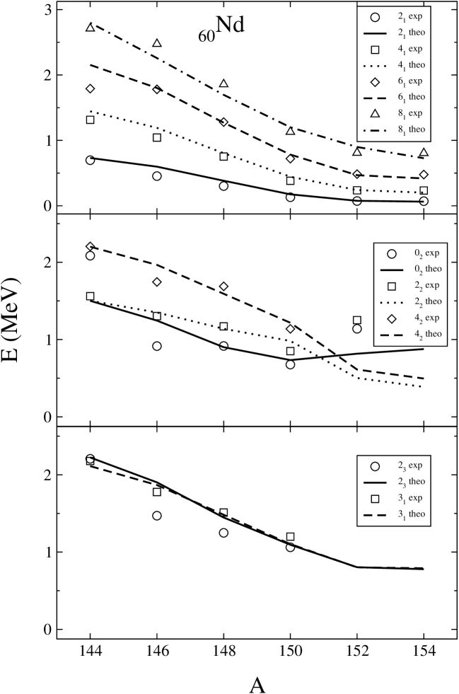
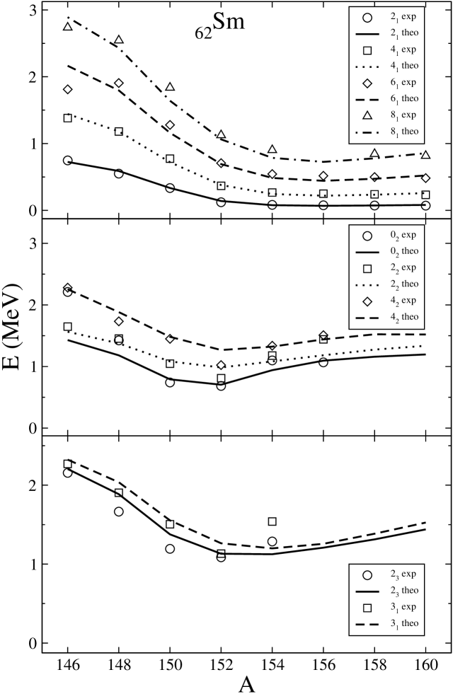
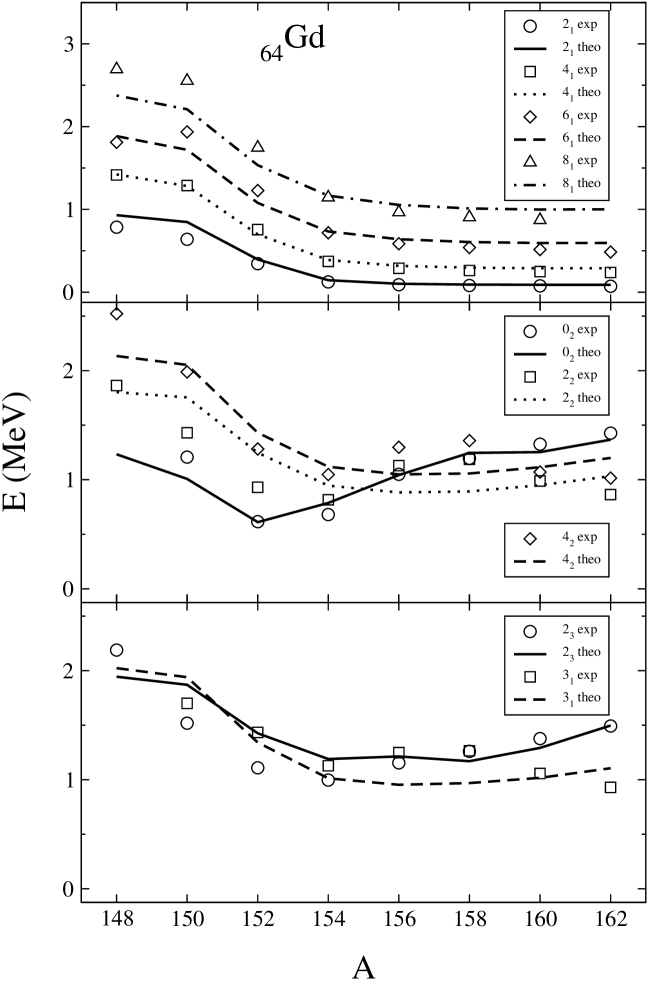
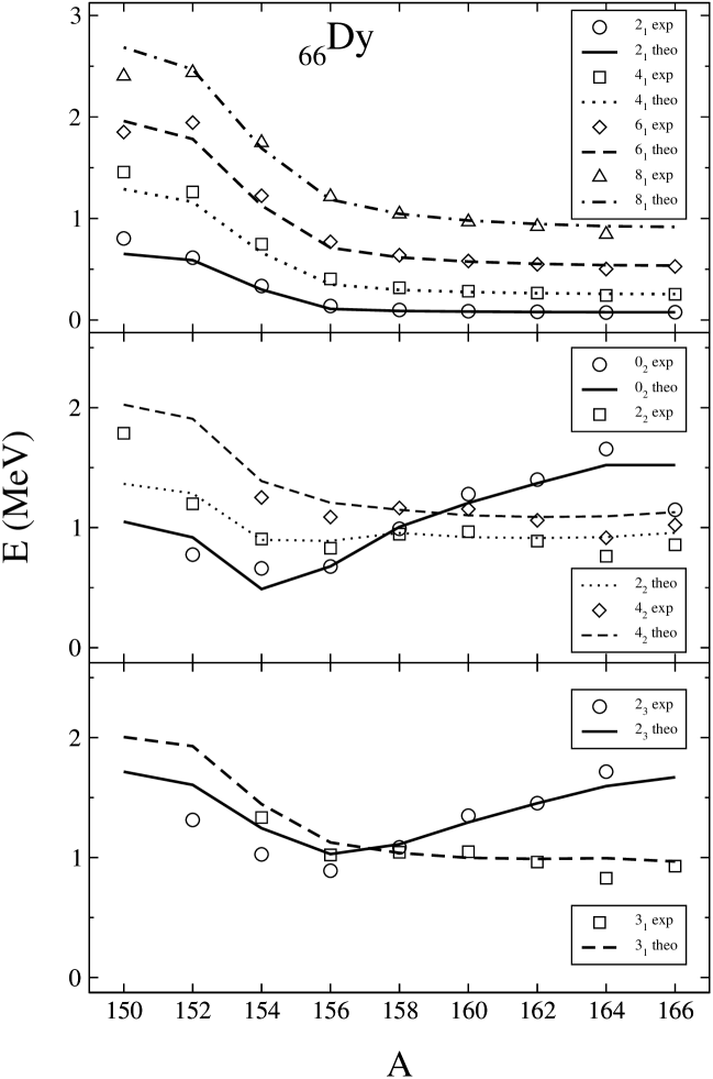
In this section we analyze several isotope chains belonging to the rare-earth region using the most general IBM Hamiltonian, Eq. (1), and $E2$ transition operator, Eq. (7). As an ansazt for each chain of isotopes we will assume a single Hamiltonian, and a single $E2$ transition operator. All parameters in these operators are kept fixed for a given isotope chain, except for the single particle energy which is allowed to vary slightly from isotope to isotope. The way of fixing the best set of parameters in the Hamiltonian is to carry out a least-square fit procedure of the excitation energies of selected states ($2^{+}_{1}$, $4^{+}_{1}$, $6^{+}_{1}$, $8^{+}_{1}$, $0^{+}_{2}$, $2^{+}_{3}$, $4^{+}_{3}$, $2^{+}_{2}$, $3^{+}_{1}$, and $4^{+}_{2}$) and the two neutron separation energies of all isotopes in each isotopic chain. Once the parameters in the Hamiltonian are obtained, the $B(E2)$ transition probabilities $2^{+}_{1}\rightarrow 0^{+}_{1}$, $4^{+}_{1}\rightarrow 2^{+}_{1}$, $2^{+}_{2}\rightarrow 0^{+}_{1}$, $2^{+}_{3}\rightarrow 0^{+}_{1}$, $0^{+}_{2}\rightarrow 2^{+}_{1}$, and $0^{+}_{3}\rightarrow 2^{+}_{1}$ of the set of isotopes are used to fix $e_{eff}$ and $\chi$ by carrying out a least-square fit. The experimental data for excitation and binding energies and B(E2)’s have been taken from Refs.  Sonz01 ; Peke97 ; Bhat00 ; Derm95 ; Artn96 ; Reic98 ; Helm92 ; Helm96 ; Reich96 ; Helm99 ; Balr01 ; Shur92 ; Audi95 . Finally, it is worth noting that in Ref. Foss02a the Hamiltonian parameters were fixed just using the data for excitation energies and then ${\cal A}$ and ${\cal B}$ were adjusted to reproduce the experimental values of S_2n. In this paper, since we are particularly interested in accurately describing the spectroscopic data associated to shape transitions, both, excitation and binding energies, are treated on an equal footing describing the shape transition, to determine the set of Hamiltonian parameters in Eq. (1).

Tables 1 and 2 summarize the parameters obtained for the Hamiltonian and $E2$ transition operator for each isotope chain.

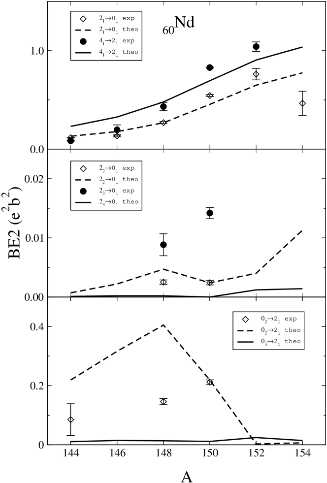
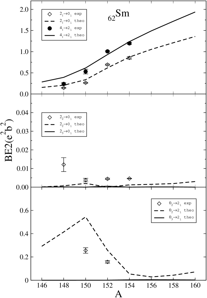
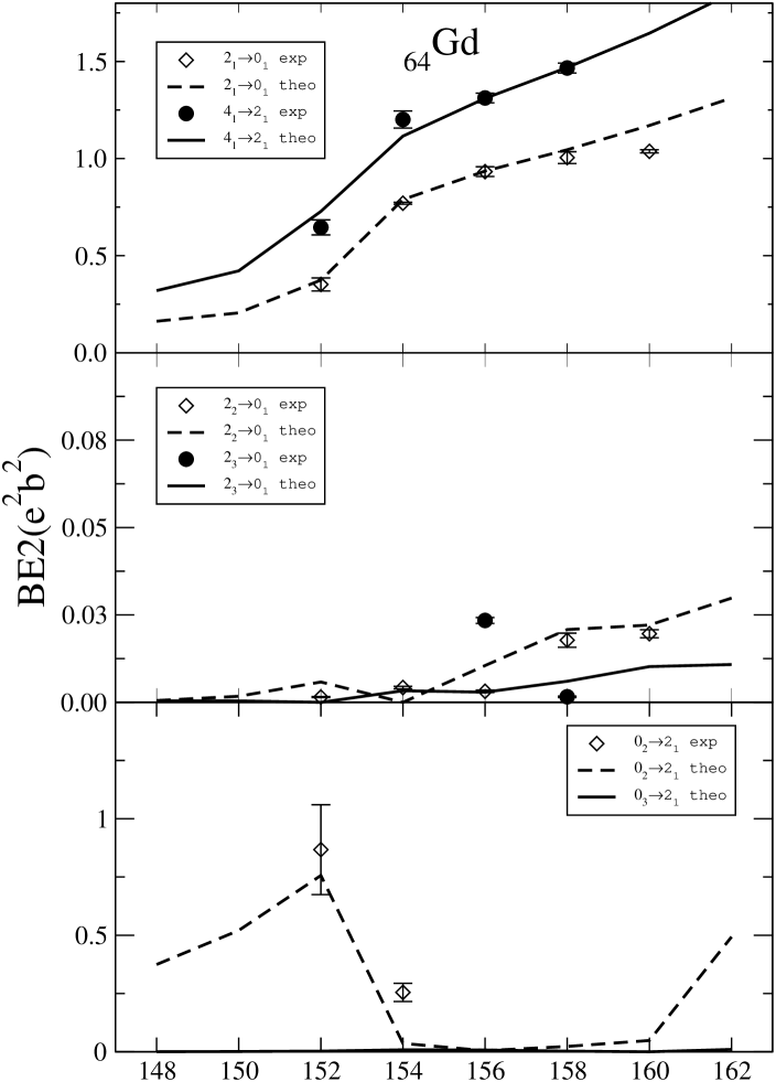
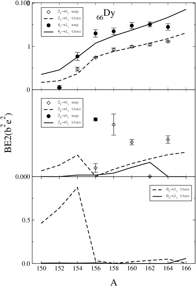
In figures 1, 2, 3, and 4 the systematics of experimental and calculated energies for the states included in the least-square procedure are presented in order to show the goodness of the fitting procedure. In figures 5, 6, 7, and 8 the systematics of the experimental and calculated $B(E2)$ values are compared. Finally, in figure 9 the experimental and calculated S_2n values are shown. This is a fundamental magnitude for identifying a phase transition since it is directly related to the derivative of the energy surface. First order phase transitions are related with the appearance of a kink in the S_2n values. As shown in Fig. 9, the calculation matches the experimentally observed behavior.

The analysis of the preceding figures for different observables and for several isotope chains shows that the present procedure is appropriate for systematic studies and confirms that it provides a simple framework to describe long chains of isotopes and detect possible phase transitions.

An alternative approach to describe long chains of rare-earth nuclei is to use the CQF. The CQF Hamiltonian is

$$\hat{H}=\epsilon\hat{n}_{d}+\kappa\hat{Q}^{\prime}\cdot\hat{Q}^{\prime}~{},$$ (10)

with

$$\hat{Q}^{\prime}=(s^{\dagger}\times\tilde{d}+d^{\dagger}\times\tilde{s})^{(2)}+\chi(d^{\dagger}\times\tilde{d})^{(2)}.$$ (11)

For each nucleus the parameters $\epsilon$, $\kappa$ and $\chi$ are determined in order to fit the excitation energies and B(E2)’s. In particular in Ref. Chou97 the parameters of the Hamiltonian are calculated within the CQF framework with the ansazt that the strength of the quadrupole term of the Hamiltonian remains constant along a wide region of the mass table. As in the present paper they compare experimental data and theoretical values for excitation energies and $B(E2)$ transition rates. Both methods provide a consistent description of the rare-earth region with a similar number of parameters as can be observed in Fig. 10 and in table 3 where the case of ¹⁵²Sm is analyzed. Note that in the present work the results come from a global analysis, therefore the $B(E2)$ transition rates are not normalized to the transition $B(E2:2_{1}^{+}\rightarrow 0_{1}^{+})$ in a particular isotope. If in table 3 the results are normalized so as to reproduce the observed value for $B(E2:2_{1}^{+}\rightarrow 0_{1}^{+})$ in ¹⁵²Sm the results of this work and CQF are basically the same.

IV Energy surfaces and phase transitions

The study of phase transitions in the IBM requires the use of the so called intrinsic-state formalism Gino80 ; Diep80 ; Diep80b , although other approaches can be used Cast99 ; Cejn00 . This formalism is very useful to discuss phase transitions in finite systems because it provides a description of the behavior of a macroscopic system up to $1/N$ effects. To define the intrinsic, or coherent, state it is assumed that the dynamical behavior of the system can be described in terms of independent bosons (“dressed bosons”) moving in an average field Duke84 . The ground state of the system is a condensate, $|c\rangle$, of bosons occupying the lowest–energy phonon state, $\Gamma^{\dagger}_{c}$,

$$|c\rangle={1\over\sqrt{N!}}(\Gamma^{\dagger}_{c})^{N}|0\rangle,$$ (12)

where

$$\Gamma^{\dagger}_{c}={1\over\sqrt{1+\beta^{2}}}\left(s^{\dagger}+\beta\cos\gamma\,d^{\dagger}_{0}+{1\over\sqrt{2}}\beta\sin\gamma\,(d^{\dagger}_{2}+d^{\dagger}_{-2})\right)$$ (13)

and $\beta$ and $\gamma$ are variational parameters related with the shape variables in the geometrical collective model. The expectation value of the Hamiltonian in the intrinsic state (12) provides the energy surface of the system, $E(N,\beta,\gamma)=\langle c|\hat{H}|c\rangle$. The energy surface in terms of the parameters of the Hamiltonian (1) and the shape variables can be readily obtained Isac81 ,

$$\langle c|\hat{H}|c\rangle = {\displaystyle{N\beta^{2}\over{(1+\beta^{2})}}}\Bigl{(}\varepsilon_{d}+6\,\kappa_{1}-{9\over 4}\,\kappa_{2}+{7\over 5}\,\kappa_{3}+{9\over 5}\,\kappa_{4}\Bigr{)}$$

$$+ {\displaystyle{\frac{N(N-1)}{{{(1+\beta^{2})}^{2}}}}}\Big{[}\frac{\kappa_{0}}{4}+\beta^{2}(-\frac{\kappa_{0}}{2}+4\,\kappa_{2})+2\,{\sqrt{2}}\,\beta^{3}\,\kappa_{2}\,\cos(3\,\gamma)$$

$$+\beta^{4}(\frac{\kappa_{0}}{4}+\frac{\kappa_{2}}{2}+\frac{18}{35}\,\kappa_{4})\Big{]},$$ (14)

where the terms which do not depend on $\beta$ and/or $\gamma$ (corresponding to $\tilde{\cal A}$ and $\tilde{\cal B}$ in Eq. (1)) have not been included.

The equilibrium values of the variational parameters $\beta$ and $\gamma$ are obtained by minimization of the ground state energy $\langle c|\hat{H}|c\rangle$. As mentioned above these parameters are related to the parameters of the Geometrical Collective Model and provide an image of the nuclear shape for a given IBM Hamiltonian. A spherical nucleus has a minimum in the energy surface at $\beta=0$, while for a deformed one the energy surface has a minimum at a finite value of $\beta$ and $\gamma=0$ (prolate nucleus) or $\gamma=\pi/3$ (oblate nucleus). Finally, a $\gamma$-unstable nucleus corresponds to the case in which the energy surface has a minimum at a particular value of $\beta$ and is independent of the value of $\gamma$. The equilibrium values of $\beta$ and $\gamma$ are the order parameters to study the phase transition of the system, although in the case under consideration (IBM-1) only $\beta$ has to be taken into account, since the minima in $\gamma$ are well defined.

In Fig. 11 the energy surfaces for the isotopes of the different isotope chains studied in this paper are plotted as a function of $\beta$. The figure on the right is a zoom of the region close to $\beta=0$.

The classification of phase transitions that we follow in this paper and that is followed traditionally in the IBM is the Ehrenfest classification Stan71 . In this context, the origin of a phase transition resides in the way the energy surface (their minima positions) is changing as a function of the control parameter that, in this work, is a combination of parameters of the Hamiltonian (see Eq. (21)). First order phase transitions appear when there exists a discontinuity in the first derivative of the energy with respect to the control parameter. This discontinuity appears when two degenerate minima exist in the energy surface for two values of the order parameter $\beta$. Second order phase transitions appear when the second derivative of the energy with respect to the control parameter displays a discontinuity. This happens when the energy surface presents a single minimum for $\beta=0$ and the surface satisfies the condition ${\left(d^{2}E\over d\beta^{2}\right)_{\beta=0}}=0$.

With the introduction of the $E(5)$ and $X(5)$ symmetries to describe phase transitional behavior, diverse attempts to identify nuclei that could be located at the critical points have been made. The theoretical approaches have been mainly performed with restricted IBM Hamiltonians. In particular, within the CQF, or other restricted Hamiltonians, the location of the critical point is obtained by imposing ${d^{2}E\over d\beta^{2}}=0$ at $\beta=0$, where $E$ is the energy surface Iach98 . This condition leads to a flat surface in a region of small values of $\beta$, with a single minimum in the limit $\chi=0$ and two almost degenerate minima (one of them in $\beta=0$) in the other cases. In the CQF approximation it can be said that ${\left(d^{2}E\over d\beta^{2}\right)_{\beta=0}}=0$ corresponds approximately to a “very flat energy surface” as happens for the $E(5)$ and $X(5)$ critical point models. Following this approach both ¹⁵⁰Nd and ¹⁵²Sm have been found to be close to critical. However, when studying a transitional region in which the lighter nuclei are spherical and the heavier are well deformed, the a priori restriction of the parameter space could play a crucial role in the identification of a particular isotope as critical. It is thus important to perform a general analysis in order to check whether the predictions obtained within the CQF for those nuclei close to a critical point are robust. We present below such an analysis in the region of the rare-earths. We follow closely the approach introduced in Ref. Lope96 ; Lope98 using catastrophe theory. In the next subsection the main ingredients of the theory are summarized and the relevant equations are particularized for the IBM Hamiltonian written in multipolar form, Eq. (1).

IV.1 The separatrix plane

For the study of phase transitions in the IBM within the framework of catastrophe theory we already have the basic ingredients: the Hamiltonian of the system, Eq. (1), and the intrinsic state, Eq. (12). With them, we have generated the corresponding energy surface, Eq. (IV), in terms of the Hamiltonian parameters and the shape variables. It is our purpose to find the values of the parameters of the Hamiltonian that correspond to critical points. In principle this analysis involves the $6$ parameters of the Hamiltonian, but a first simplification occurs since the energy surface only depends on $5$ parameters :

$$\langle c|\hat{H}|c\rangle = {N\tilde{\varepsilon}\beta^{2}\over{(1+\beta^{2})}}+{N(N-1)\over(1+\beta^{2})^{2}}\Big{(}a_{1}\beta^{4}+a_{2}\beta^{3}\cos(3\,\gamma)+a_{3}\beta^{2}+{u_{0}\over 2}\Big{)},$$ (15)

where

$$\tilde{\varepsilon} = \varepsilon_{d}+6\,\kappa_{1}-{9\over 4}\,\kappa_{2}+{7\over 5}\,\kappa_{3}+{9\over 5}\,\kappa_{4}$$

$$a_{1} = {1\over 4}\,\kappa_{0}+{1\over 2}\,\kappa_{2}+{18\over 35}\,\kappa_{4}$$

$$a_{2} = 2\,\sqrt{2}\,\kappa_{2}$$

$$a_{3} = -{1\over 2}\,\kappa_{0}+4\,\kappa_{2}$$

$$u_{0} = {\kappa_{0}\over 2}.$$ (16)

Fortunately, it is possible to reduce the number of relevant (or essential) parameters to just two and study all phase transitions by using catastrophe theory Gilm81 . We refer the reader to Refs. Lope96 ; Lope98 for details of the application of this theory to the IBM case. The idea is to analyze the energy surface and obtain all equilibrium configurations, i.e. to find all the critical points of Eq. (15). First, the critical point of maximum degeneracy has to be identified. In our case, it corresponds to $\beta=0$. Next, the bifurcation and Maxwell sets are constructed Gilm81 ; Lope96 . Finally, the separatrix of the IBM is obtained by the union of Maxwell and bifurcation sets. In general a bifurcation set, corresponding to minima, limits an area where two minima in the energy surface coexist. A second order phase transition develops when these minima become the same. The crossing of a Maxwell set corresponding to minima leads to a first order phase transition.

In order to follow this scheme, one has to identify the catastrophe germ of the IBM, which is the first term in the expansion of the energy surface around the critical point of maximum degeneracy that cannot be canceled by an arbitrary selection of parameters. In our case, one finds that the first derivative in $\beta=0$ is always $0$ because of the critical character of the point for any value of the parameters. The second and third derivatives can also be canceled with an appropriate selection of parameters. However, if one imposes the cancellation of the fourth derivative, the energy becomes a constant for any value of $\beta$. This means that the catastrophe germ is $\beta^{4}$ and the number of essential parameters is equal to two, which can be defined, following reference Lope96 ; Lope98 , as

$$r_{1}={a_{3}-u_{0}+\tilde{\varepsilon}/(N-1)\over 2a_{1}+\tilde{\varepsilon}/(N-1)-a_{3}},$$ (17)

$$r_{2}=-{2a_{2}\over 2a_{1}+\tilde{\varepsilon}/(N-1)-a_{3}},$$ (18)

where $\tilde{\varepsilon}$, $a_{1}$, $a_{2}$, and $a_{3}$ are defined in (16). The denominator in both expressions fixes the energy scale, which means that when it becomes negative, the energy surfaces are inverted. The essential parameters $r_{1}$ and $r_{2}$ can also be written in terms of the parameters appearing in (1) as ,

$$r_{1}={\tilde{\varepsilon}-(N-1)(\kappa_{0}-4\kappa_{2})\over\tilde{\varepsilon}+(N-1)(\kappa_{0}-3\kappa_{2}+\frac{36}{35}\kappa_{4})},$$ (19)

$$r_{2}=-{4\sqrt{2}\kappa_{2}(N-1)\over\tilde{\varepsilon}+(N-1)(\kappa_{0}-3\kappa_{2}+\frac{36}{35}\kappa_{4})}.$$ (20)

A property of the parametrization used in this work is that the different chains of isotopes are located on a straight line that crosses the point corresponding to the $U(5)$ limit. The equation of this line is given by

$$r_{1}={2\kappa_{0}-7\kappa_{2}+{36\over 35}\kappa_{4}\over 4\sqrt{2}\kappa_{2}}r_{2}+1$$ (21)

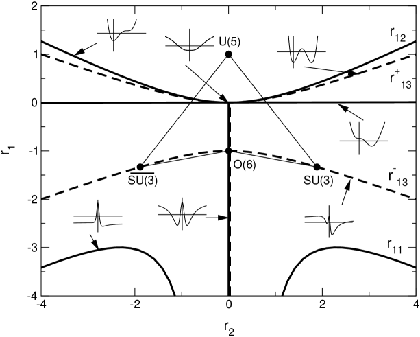
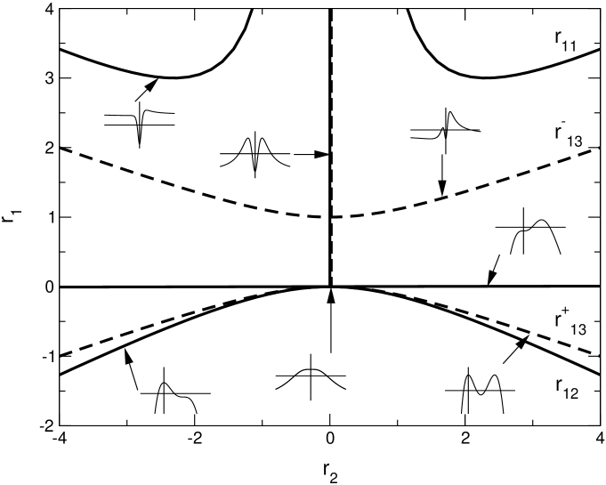
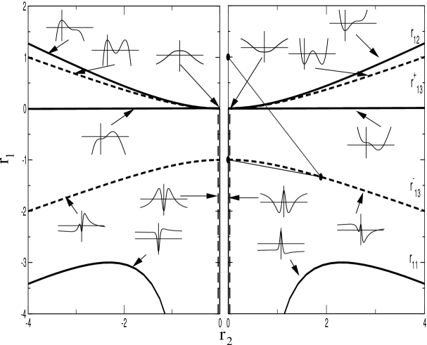
It should be remarked that the derivation of the essential parameters has nothing to do with catastrophe theory. The application of this theory begins once those parameters are obtained. The basic point is to translate every set of Hamiltonian parameters to the plane formed by the essential parameters $r_{1}$ and $r_{2}$. This plane is divided into several sectors by the bifurcation set, that form the geometrical place in the parameter space where ${d^{2}E\over d\beta^{2}}=0$ for a critical value of $\beta$, and the Maxwell sets, the geometrical place in the space of parameters where two or more critical points are degenerate Gilm81 . Both sets form the separatrix of the system, in this case of the IBM. In Ref. Lope96 ; Lope98 the IBM bifurcation ($r_{2}$ axis, $r_{2}=0$ and $r_{1}<0$ semi-axis, $r_{11}$, and $r_{12}$) and Maxwell (negative $r_{1}$ semi-axis, $r_{13}^{+}$, and $r_{13}^{-}$) sets were obtained. They are all indicated in Fig. 12. In this representation it is required that the denominator in (17) and (18) is positive. The separatrix for $r_{1}>0$ is associated to minima while for $r_{1}<0$ is associated to maxima (except the negative $r_{1}$ semi-axis). In order to clarify the figure on the separatrix, the energy surfaces corresponding to each set are plotted as insets. The half plane with $r_{2}>0$ corresponds to prolate nuclei, while the one with $r_{2}<0$ corresponds to oblate nuclei. Note that expressions (19) and (20) are only valid for prolate nuclei, but can be readily obtained for the oblate case. On this figure the symmetry limits and the correspondence with Casten’s triangle Iach87 are also represented. For completeness one should consider the case where the denominator of (17) and (18) is negative. It implies that the energy scale becomes negative and the energy surface should be inverted. The separatrix for this case is plotted in figure 13 and corresponds to the inversion of figure 12. Again the schematic energy surfaces corresponding to each branch of the separatrix are shown as insets. Note that in this case the symmetry limits do not appear in the figure because they correspond to positive denominators for $r_{1}$ and $r_{2}$. In our analysis only prolate nuclei are considered, because of that a new figure, Fig. 14, is included. In this figure, the right panel corresponds to positive denominators for $r_{1}$ and $r_{2}$ while the left panel shows the case of negative denominator for $r_{1}$ and $r_{2}$. In the following we will follow the convention presented in this figure.

A set of parameters in the Hamiltonian corresponds to a point in the separatrix plane. The location of the point in that plane provides the required information on its transitional phase character. As mentioned above, it follows that points located on a separatrix line correspond to critical points. Note that the dynamical behavior of the system is controlled by the lowest minimum in the energy surface. In this sense we are adopting the Maxwell convention in the catastrophe theory language Gilm81 and the only relevant branches of the separatrix are $r_{13}^{+}$ and $r_{2}=0$ with $r_{1}\leq 0$. All these branches correspond to first order phase transitions except for the single point $(r_{1}=0,r_{2}=0)$ that corresponds to a second order phase transition. The rest of Maxwell lines do not correspond to a phase transition because they are related to maxima. The interest of the bifurcation set, corresponding to minima, arises from the fact that it defines regions where two minima exits. In the following subsection the transitional isotope chains studied in this paper are analyzed in the separatrix plane.

IV.2 Rare-earth region on the separatrix plane

The fits presented in Sect. III provide the parameter sets given in Tables 1 and 2 for the four isotope chains studied in this paper. In this section we plot the corresponding sequences of points representing the isotopes in each chain on the separatrix plane. As can be observed in the previous tables all the parameters for each chain are fixed except the value of $\varepsilon_{d}$ that changes along the chain.

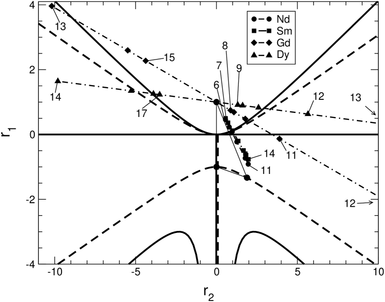
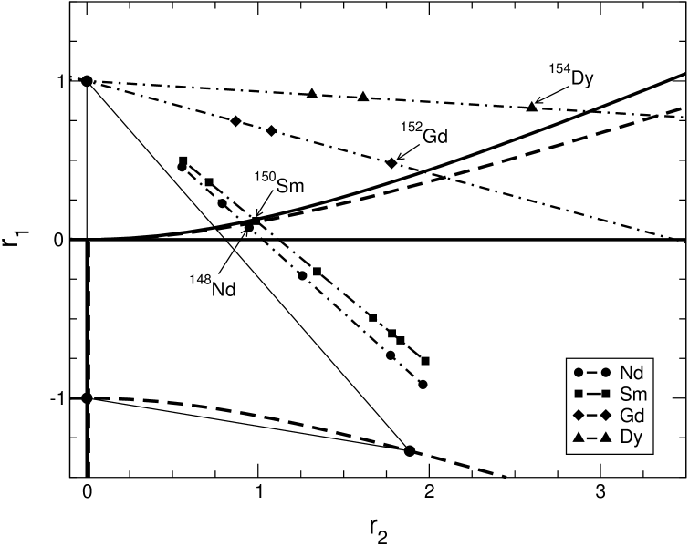
In figure 15 the positions of the different isotopes in the chains studied are plotted in the separatrix plane. The interpretation of these lines is given in Fig. 14. As mentioned above, all isotopes in a chain lie on a straight line. The lighter ones are close to the $U(5)$ point (spherical shapes) while as the number of neutrons is increased the corresponding points get increasingly away. For the heavier isotopes of Gd, and Dy the denominator of $r_{1}$ and $r_{2}$ becomes negative, which means that the left panel in Fig. 14 has to be used.

The main feature we find is that some nuclei are close to the Maxwell set $r_{13}^{+}$: the closest are ¹⁴⁸Nd (boson number $N=8$) and ¹⁵⁰Sm (boson number $N=9$) and not far away ¹⁵²Gd (boson number $N=10$). This can be complemented with the image of the energy surfaces plotted in Fig. 11. The energy surface for ¹⁴⁸Nd and ¹⁵⁰Sm are rather flat around $\beta=0$. For ¹⁵²Gd the situation is not so clear. For Dy there is no isotope close to the critical point. According to our calculations, the transition from spherical to deformed occurs between $N=11$ and $N=12$. The isotope ¹⁶²Dy is close to the Maxwell set but in the left panel. In this situation there should be two degenerate maxima. This can be observed in the corresponding energy surface (boson number $N=15$) in Fig. 11. The isotopes ¹⁵⁰Nd ($N=9$) and ¹⁵²Sm ($N=10$) (also can be included in this situation ¹⁵⁴Gd ($N=11$) and ¹⁵⁸Dy ($N=13$)) are close to the bifurcation set $r_{2}$ axis. Again inspection of Fig. 11 shows that the energy surfaces for these isotopes has a minimum for $\beta>0$ and a maximum at $\beta=0$. In figure 16 we show an amplification of the critical area.

In conclusion, from this global analysis we find that ¹⁴⁸Nd, ¹⁵⁰Sm, and (less clearly) ¹⁵²Gd, are close to criticality. These isotopes are quite close but do not exactly coincide with previously proposed critical nuclei ¹⁵⁰Nd and ¹⁵²Sm Cast01 ; Kruc02 , where the quite basic criterion was the closeness of their low-lying excitation spectra and transition intensities with the $X(5)$ values.

IV.3 Prediction of critical points within CQF

The CQF uses a simplified Hamiltonian with only three parameters. For the description of transitional nuclei from the $U(5)$ to the $SU(3)$ limits the parameters are allowed to vary nucleus by nucleus. The representation of such calculations in the separatrix plane shows that all isotopes in a chain are basically on top of the straight line connecting the $U(5)$ point, $(r_{1},r_{2})=(1,0)$, and the $SU(3)$ point, $(r_{1},r_{2})=(-4/3,4\sqrt{2}/3)$. Note that this point corresponds strictly to the $SU(3)$ Casimir operator. However, a more general CQF $SU(3)$ Hamiltonian still lies very close to the latter point. In general, the same happens in the $U(5)$ and $O(6)$ points. This means that within this framework the exploration of only a limited area in the separatrix plane is allowed. If all isotopes in an isotopic chain are forced to be located on the line connecting the $U(5)$ and $SU(3)$ points, it follows that one will more often find an isotope close to the (unique) critical point. In the calculations presented here we have seen that within the general formalism this is not always the case. For example, for Dy we did not find an isotope close to a critical point.

In previous systematic studies in the rare-earth region using the CQF formalism, Ref. Chou97 and Foss02a , the corresponding energy surfaces were not presented. We have constructed them from the parameters given in those references and the results obtained are consistent with those given in the present work. In particular, ¹⁴⁸Nd and ¹⁵⁰Sm seem to be closest to a critical point.

V Conclusions

In this paper we have analyzed chains of isotopes in the rare-earth region. In these chains nuclei evolve from spherical to deformed shapes. We have performed an analysis of the corresponding shape transitions to look for possible nuclei at or close to a critical point. We have used the more general one- and two- body IBM Hamiltonian and generated energy surfaces using the coherent state formalism. We have then used catastrophe theory to classify phase transitions and to decide if a nucleus is close to criticality.

The approach used to fix the Hamiltonian parameters leads to a very good global agreement with the experimental data corresponding to excitation energies, B(E2)’s and S_2n values. In particular, an excellent agreement with the measured S_2n values is obtained, which is considered a key observable to locate phase transitional regions. The analysis presented here is consistent with previous CQF studies in the same region. As a result we find that ¹⁴⁸Nd and ¹⁵⁰Sm are the best candidates to be critical, but we should remark that ¹⁵⁰Nd and ¹⁵²Sm are not far away from it.

A possible new way of defining critical nuclei is based on the “critical symmetries” $E(5)$ or $X(5)$ Iach00 ; Iach01 . The properties associated with these solutions allow the identification of critical points by comparing the experimental data with characteristic energy and transition rate ratios. Thus, it may be possible to decide whether a nucleus is critical by analyzing its spectrum and decay properties. A trickier question is whether a flat energy surface can be truly associated to a given nucleus with energy ratios close to $X(5)$. A clear example is ¹⁵²Sm: in section IV.2 we have shown that according to our study the IBM energy surface of this nucleus is not so flat as expected from previous analyses, i.e. in our work it does not correspond to a critical point as suggested earlier. However, if the spectrum and transition rates are analyzed (see figure 10 and table 3 ), this nucleus reproduces reasonably well the main $X(5)$ features. We note that in the general IBM framework there is no unique spectrum associated to a given potential energy surface, as implied by equations (17) an (18). Catastrophe theory constitutes a definite criterion regarding this issue, but does not provide a measurable signature in itself.

It seems clear that further work is required to find experimentally identifiable features which signal criticality in an unequivocal way.

VI Acknowledgements

We acknowledge insightful discussions with R.F. Casten, F. Iachello, K. Heyde, J. Jolie, P. Van Isacker, and P. Von Brentano. This work was supported in part by the Spanish DGICYT under projects number FPA2000-1592-C03-02 and BFM2002-03315 and by CONACYT (México).

Table 1: Values of $\varepsilon_{d}$ in the Hamiltonian (in keV) for each isotopic chain as a function of the neutron number.

	Neutron Number
Element	84	86	88	90	92	94	96	98	100
60Nd	1686.3	1606.7	1645.4	1602.9	1536.1	1595.9
62Sm	1427.3	1393.5	1289.3	1210.8	1158.6	1192.5	1312.2	1452.0
64Gd	1479.3	1508.7	1409.0	1300.4	1221.5	1174.4	1162.0	1176.5
66Dy	1558.8	1607.6	1562.4	1503.9	1461.0	1427.7	1413.4	1409.2	1443.1

Table 2: Rest of the parameters in the Hamiltonian and in the E2 transition operator.

Isotopes	$\tilde{\cal A}$ (MeV)	$\tilde{\cal B}$ (MeV)	$\kappa_{0}$ (keV)	$\kappa_{1}$ (keV)	$\kappa_{2}$(keV)	$\kappa_{3}$ (keV)	$\kappa_{4}$ (keV)	$e_{eff}$ ($e\cdot b$)	$\chi$
${}^{144-154}_{\phantom{4-154}60}$Nd	16.75	-0.51	83.753	-13.928	-17.151	-101.27	-187.57	0.119	-1.43
${}^{146-160}_{\phantom{4-154}62}$Sm	18.05	-0.46	53.209	-11.267	-14.674	-31.769	-131.24	0.119	-1.69
${}^{148-162}_{\phantom{4-154}64}$Gd	22.55	-0.76	45.207	-7.932	-13.129	-35.224	-156.24	0.110	-1.77
${}^{150-166}_{\phantom{4-154}66}$Dy	25.06	-0.80	38.651	-6.416	-13.638	-59.165	-163.05	0.103	-1.60

Table 3: Relevant transition rates for ¹⁵²Sm (in w.u.).

	Exp.	$X(5)$	This work	CQF(a)
$B(E2:2_{1}^{+}\rightarrow 0_{1}^{+})$	144	144	128	144
$B(E2:4_{1}^{+}\rightarrow 2_{1}^{+})$	209	228	193	216
$B(E2:6_{1}^{+}\rightarrow 4_{1}^{+})$	245	285	215	242
$B(E2:8_{1}^{+}\rightarrow 6_{1}^{+})$	285	327	218	248
$B(E2:10_{1}^{+}\rightarrow 8_{1}^{+})$	320	376	210	242
$B(E2:0_{2}^{+}\rightarrow 2_{1}^{+})$	33	91	53	57
$B(E2:2_{2}^{+}\rightarrow 4_{1}^{+})$	19	52	14	20
$B(E2:2_{2}^{+}\rightarrow 2_{1}^{+})$	6	13	5	11
$B(E2:2_{2}^{+}\rightarrow 0_{1}^{+})$	1	3	0	0.1
$B(E2:4_{2}^{+}\rightarrow 6_{1}^{+})$	4	40	7	14
$B(E2:4_{2}^{+}\rightarrow 4_{1}^{+})$	5	9	2	8
$B(E2:4_{2}^{+}\rightarrow 2_{1}^{+})$	1	13	0	0.1

^(a) Following Ref. Iach98 .

Figure 1: Excitation energies of Nd isotopes.

Figure 2: Excitation energies of Sm isotopes.

Figure 3: Excitation energies of Gd isotopes.

Figure 4: Excitation energies of Dy isotopes.

Figure 5: $B(E2)$ transition rates for Nd isotopes.

Figure 6: $B(E2)$ transition rates for Sm isotopes.

Figure 7: $B(E2)$ transition rates for Gd isotopes.

Figure 8: $B(E2)$ transition rates for Dy isotopes.

Figure 9: S_2n values for Nd, Sm, Gd, and Dy isotopes.

Figure 10: Spectrum of ¹⁵²Sm: (a) experimental, (b) X(5) symmetry, (c) this work, and (d) using CQF Iach98 .

Figure 11: Energy surfaces for the different chain of isotopes.

Figure 12: Separatrix plane with a positive energy scale.

Figure 13: Separatrix plane with a negative energy scale.

Figure 14: Separatrix plane for prolate nuclei ($\chi<0$).

Figure 15: Representation of isotopes in the separatrix plane (with $\chi<0$).The numbers on the isotopes correspond to the number of bosons.

Figure 16: Representation of isotopes in the separatrix plane in a closest view.

References

- (1) D.J. Rowe, C. Bahri, and W. Wijesundera, Phys. Rev. Lett. 80, 4394, (1998).
- (2) F. Iachello, N.V. Zamfir, and R.F. Casten, Phys. Rev. Lett. 81, 1191, (1998).
- (3) R.F. Casten, D. Kusnezov, and N.V. Zamfir, Phys. Rev. Lett. 82, 5000, (1999).
- (4) J. Jolie, P. Cejnar, and J. Dobes̆, Phys. Rev. C 60, 061303, (1999).
- (5) F. Iachello, Phys. Rev. Lett. 85, 3580, (2000).
- (6) F. Iachello, Phys. Rev. Lett. 87, 052502, (2001).
- (7) F. Iachello and A. Arima. “The interacting boson model”. Cambridge University Press, Cambridge, (1987).
- (8) J. Jolie, R.F. Casten, P. von Brentano and V. Werner, Phys. Rev. Lett. 87, 162501, (2001).
- (9) O. Castaños, A. Frank and P. Federman, Phys. Lett. 88B, 203, (1979).
- (10) O. Castaños, P. Federman, A. Frank, and S. Pittel, Nucl. Phys. A 379, 61, (1982).
- (11) A. Frank, Phys. Rev. C 39, 652, (1989).
- (12) A. Gómez, O. Castaños, and A. Frank, Nucl. Phys. A 589, 267, (1995). A. Gómez, O. Castaños, A. Frank, C.E. Alonso, and J.M. Arias, Nucl. Phys. A 594, 483, (1995).
- (13) D.D. Warner and R.F. Casten, Phys. Rev. Lett. 48, 1385, (1982).
- (14) E. López-Moreno and O. Castaños, Phys. Rev. C 54, 2374, (1996).
- (15) E. López-Moreno, PhD thesis, Universidad Nacional Autónoma de México, 1998, unpublished.
- (16) R. Gilmore. “Catastrophe theory for scientists and engineers”. Wiley, New York, (1981).
- (17) N.V. Zamfir et al, Phys. Rev. C 60, 054312 (1999).
- (18) R.F. Casten and N.V. Zamfir, Phys. Rev. Lett. 85, 3584, (2000).
- (19) T. Klug, A. Dewald, V. Werner, P. von Brentano and R.F. Casten, Phys. Lett. B 495, 55 (2000).
- (20) R.F. Casten and N.V. Zamfir, Phys. Rev. Lett. 87, 052503, (2001).
- (21) A. Frank, C.E. Alonso, and J.M. Arias, Phys. Rev. C 65, 014301, (2001).
- (22) N.V. Zamfir et al, Phys. Rev. C 65, 044325, (2002).
- (23) B.G. Bizzeti and A.M. Bizzeti-Sona, Phys. Rev. C 66, 031301, (2002).
- (24) R. Krücken et al, Phys. Rev. Lett. 88, 232501, (2002)
- (25) R. Fossion, C. De Coster, J.E. García-Ramos, T. Werner, and K. Heyde, Nucl. Phys. A 697, 703, (2002).
- (26) A.A. Sonzogni, Nucl. Data Sheets 93, 599, (2001).
- (27) L.K. Peker and J.K. Tuli, Nucl. Data Sheets 82, 187, (1997).
- (28) M.R. Bhat, Nucl. Data Sheets 89, 797, (2000).
- (29) E. Dermateosian and J.K Tuli, Nucl. Data Sheets 75, 827, (1995).
- (30) Agda Artna-Cohen, Nucl. Data Sheets 79, 1, (1996).
- (31) C.W. Reich and R.G. Helmer, Nucl. Data Sheets 85, 171, (1998).
- (32) R.G. Helmer, Nucl. Data Sheets 65, 65, (1992).
- (33) R.G. Helmer, Nucl. Data Sheets 77, 471, (1996).
- (34) C.W. Reich, Nucl. Data Sheets 78, 547, (1996).
- (35) R.G. Helmer and C.W. Reich, Nucl. Data Sheets 87, 317, (1999).
- (36) Balraj Singh, Nucl. Data Sheets 93, 243, (2001).
- (37) E.N. Shurshikov and N.V. Timofeeva, Nucl. Data Sheets 67, 45, (1992).
- (38) G. Audi and A.H. Wapstra, Nucl. Phys. A 595, 409, (1995).
- (39) W.-T. Chou, N.V. Zamfir, and R.F. Casten, Phys. Rev. C 56, 829, (1997).
- (40) J.N. Ginocchio and M.W. Kirson, Nucl. Phys. A 350, 31, (1980).
- (41) A.E.L. Dieperink and O. Scholten, Nucl. Phys. A 346, 125, (1980).
- (42) A.E.L. Dieperink, O. Scholten, and F. Iachello, Phys. Rev. Lett. 44, 1747, (1980).
- (43) P. Cejnar and J. Jolie, Phys. Rev. E 61, 6237, (2000).
- (44) J. Dukelsky, G.G. Dussel, R.P.J. Perazzo, S.L. Reich, and H.M. Sofia, Nucl. Phys. A 425, 93, (1984).
- (45) P. Van Isacker and J.Q. Chen, Phys. Rev. C 24 684, (1981).
- (46) H.E. Standley, “Introduction to phase transitions and critical phenomena”, Oxford University Press, Oxford (1971).