Narrow Resonances in Effective Field Theory

Abstract

We discuss the power counting for effective field theories with narrow resonances near a two-body threshold. Close to threshold, the effective field theory is perturbative and only one combination of coupling constants is fine-tuned. In the vicinity of the resonance, a second, “kinematic” fine-tuning requires a nonperturbative resummation. We illustrate our results in the case of nucleon-alpha scattering.

The last ten years have seen the development of effective field theories (EFTs) for systems of few nucleons ARNPSreview ; NN99 . Nucleons in light nuclei have typical momenta that are small compared to the characteristic QCD scale of 1 GeV. At these low momenta, QCD can conveniently be represented by a hadronic theory containing all possible interactions consistent with the QCD symmetries. It is crucial to formulate a power counting that justifies a systematic and controlled truncation of the Lagrangian according to the desired accuracy. Nuclei offer a non-trivial challenge because one wants such a perturbative expansion in addition to the non-perturbative treatment of certain leading operators, which is required by the existence of shallow bound states. By now, two-, three- and four-nucleon systems have been studied with EFT. While much remains to be understood, many successes have been achieved ARNPSreview ; NN99 .

The extension of EFTs to larger nuclei faces computational challenges, as do other approaches. As a first step halos in this extension, we can specialize to very low energies where clusters of nucleons behave coherently. Even though many interesting issues of nuclear structure are avoided, we can still describe anomalously shallow (“halo”) nuclei and some reactions of astrophysical interest.

Reactions involving more complex nuclei are frequently characterized by narrow resonances near threshold. One example, the $p_{3/2}$ resonance in neutron-alpha ($n\alpha$) scattering, was considered in Ref. halos . A good description of the data throughout the resonance region was found at the expense of the resummation of two operators in addition to the unitarity cut. Such a resummation requires two fine-tunings, which is somewhat surprising. Here we generalize the analysis of shallow, narrow resonances in EFT. We discuss the power counting for resonances in any partial wave, and clarify the scope of unitarization. We again use $n\alpha$ scattering as an example, in order to make the comparison with Ref. halos explicit.

We consider a two-body scattering with reduced mass $\mu$ and energy $E=k^{2}/2\mu$ in the center-of-mass frame. Resonance behavior arises when the $S$-matrix has a pair of poles in the two lower quadrants of the complex $k$ plane. The projection of $S$ in the partial wave $l$ where the resonance lies can be written

$$S_{l} = -\frac{k+k_{+}}{k-k_{+}}\,\frac{k+k_{-}}{k-k_{-}}\,s_{l}(k)$$ (1)

$$= -\frac{E-E_{0}-i\Gamma(E)/2}{E-E_{0}+i\Gamma(E)/2}\,s_{l}(k).$$

Here $k_{\pm}=\pm k_{R}+ik_{I}$ with $k_{I}<0$ are the pole positions, $s_{l}(k)$ is a smooth function in the energy region under consideration, $E_{0}=(k_{R}^{2}+k_{I}^{2})/2\mu$ is the position of the resonance —defined as the energy where the corresponding phase shift crosses $\pi/2$— and $\Gamma(E)/2=-kk_{I}/\mu$ is referred to as the half-width of the resonance. A narrow resonance is one for which $\Gamma(E_{0})/2E_{0}\ll 1$, that is, for which the poles are near the real axis, $|k_{I}/k_{R}|\ll 1$.

We say the resonance is shallow if $|k_{\pm}|\equiv M_{lo}\ll M_{hi}$, where $M_{hi}$ is the characteristic scale of the underlying theory, such as the energy scale of excitations of the particles under consideration and the mass of exchanged particles. A physical example of a shallow, narrow resonance is the $p_{3/2}$ resonance in $n\alpha$ scattering, which in our fit halos has $\Gamma(E_{0})/2\simeq 0.3\,{\rm MeV}\ll E_{0}\simeq 0.8\,{\rm MeV}\ll E_{\alpha}\simeq 20\,{\rm MeV}$, or $k_{I}\simeq-6\,{\rm MeV}\ll k_{R}\simeq 34\,{\rm MeV}\ll\sqrt{m_{N}E_{\alpha}}\simeq 140\,{\rm MeV}$, where $E_{\alpha}$ is the excitation energy of the $\alpha$ core and $m_{N}$ is the nucleon mass. (Similar values can be found in other fits tunl .) Another example of a shallow resonance can be found in the $s$-wave channel of a two-range Gaussian potential (see, e.g., Ref. polemodels ).

Physics at a momentum scale $Q\sim M_{lo}$ can be described by an EFT containing as degrees of freedom only the scattering particles. For notational simplicity we take the two particles to be identical, with mass $m=2\mu$ and no spin. Generalization to other situations is straightforward. In an EFT, observables are independent of the choice of fields. It proves convenient to introduce a field $d$ —the “dimeron”— with the quantum numbers of the resonance halos , as can be done for a shallow $s$-wave bound state Kap97 .

Let us first consider the case where the resonance is in the $l=1$ state. The auxiliary field $d_{i}$ has spin $1$ and the Lagrangian reads,

$${\cal L}=\psi^{\dagger}\biggl{[}i\partial_{0}+\frac{\overrightarrow{\nabla}^{\,2}}{2m}\bigg{]}\psi+\eta_{1}d^{\dagger}_{i}\bigg{(}i\partial_{0}+\frac{\overrightarrow{\nabla}^{\,2}}{4m}-\Delta_{1}\bigg{)}d_{i}+\frac{g_{1}}{4}\left(d^{\dagger}_{i}\psi\tensor{\partial}_{i}\psi+{\rm H.c.}\right)+\ldots\,,$$ (2)

where the sign $\eta_{1}=\pm 1$, the parameters $g_{1}\equiv\sqrt{4\pi\alpha_{1}}$ and $\Delta_{1}$ are fixed from matching with the underlying theory or directly from the data, $\tensor{\partial}_{i}$ is a shorthand notation for $\roarrow{\partial}_{i}-\loarrow{\partial}_{i}$, and the dots represent terms with more derivatives. An EFT without the dimeron field can be obtained by performing the Gaussian path integral over $d_{i}$.

Introducing ${\tilde{k}}^{2}=mp_{0}-{\mathbf{p}}^{2}/4$, the bare propagator for a dimeron of energy $p_{0}$ and momentum ${\mathbf{p}}$ is given by

$$iD_{l}^{(0)}(p_{0},{\mathbf{p}})_{ij}=\frac{i\eta_{1}m}{{\tilde{k}}^{2}-m\Delta_{1}+i\epsilon}\,\delta_{ij}.$$ (3)

The full dimeron includes bubbles —shown diagrammatically in Fig. 1— generated by $d^{\dagger}\psi\psi$ interactions, as well as insertions stemming from terms with more derivatives. The two-particle $T$-matrix can be obtained from the full dimeron propagator by attaching external particle legs.

Figure 1: The full dimeron propagator (thick shaded line) is obtained by dressing the bare dimeron propagator (double solid line) with particle bubbles (solid lines) to all orders.

Before discussing the power counting, we compute the two-particle scattering amplitude including only the interactions explicitly shown in Eq. (2). We work in the center-of-mass frame of the two particles, where we denote the relative incoming (outgoing) momenta by ${\mathbf{k}}\;({\mathbf{k}^{\prime}})$ and the scattering angle by $\theta$. The total energy is simply $k^{2}/m$, and ${\tilde{k}}^{2}=k^{2}$. The result for the scattering amplitude is

$$T(k,\cos\theta)=\frac{12\pi}{m}k^{2}\cos\theta\left[\eta_{1}\frac{12\pi\Delta_{1}}{mg_{1}^{2}}-\frac{2L_{3}}{\pi}-k^{2}\left(\eta_{1}\frac{12\pi}{m^{2}g_{1}^{2}}+\frac{2L_{1}}{\pi}\right)-ik^{3}\right]^{-1}\,,$$ (4)

where

$$L_{n}=\int dq\,q^{n-1}$$ (5)

is an integral proportional to $\Lambda^{n}$, with $\Lambda$ an ultraviolet momentum cutoff. Matching Eq. (4) to the effective-range expansion for the scattering amplitude,

$$T(k,\cos\theta)=\frac{12\pi}{m}k^{2}\cos\theta\left[-\frac{1}{a_{1}}+\frac{r_{1}}{2}k^{2}+\ldots-ik^{3}\right]^{-1}\,,$$ (6)

the parameters $\Delta_{1}$ and $g_{1}$ in the Lagrangian (2) can be determined in terms of the effective-range parameters, for instance

$$\frac{1}{a_{1}} = \frac{2L_{3}}{\pi}-\eta_{1}\frac{12\pi\Delta_{1}}{mg_{1}^{2}}\,,$$

$$-\frac{r_{1}}{2} = \eta_{1}\frac{12\pi}{m^{2}g_{1}^{2}}+\frac{2L_{1}}{\pi}\,.$$ (7)

Dimensional analysis suggests that the typical size (in order of magnitude) for the effective-range parameters $a_{1},r_{1},\ldots$ is given by the appropriate power of the momentum scale $M_{hi}$ where the effective theory breaks down. For instance, if the interaction between the particles is described by a potential of depth $\sim M_{hi}$ and range $\sim 1/M_{hi}$, one would expect $a_{1}\sim 1/M_{hi}^{3}$ and $r_{1}\sim M_{hi}$. In particular, a resonance or bound state, if present, generally occurs at the momentum scale $M_{hi}$. These cases have already been considered in Ref. halos and we have nothing to add to it here. In some systems, however, the interactions are finely tuned in such a way as to produce a resonance close to threshold, at a scale $M_{lo}$ much smaller than $M_{hi}$, violating the naive dimensional-analysis estimate. This situation can occur when one or more of the effective-range parameters have unnatural sizes related to the low-momentum scale $M_{lo}$. In Ref. halos , the situation when $a_{1}\sim 1/M_{lo}^{3}$ and $r_{1}\sim M_{lo}$ was analyzed. Note that this requires that two combinations of constants, $\Delta_{1}/g_{1}^{2}$ and $1/g_{1}^{2}$, be fine-tuned against the large values of $L_{n}\sim(M_{hi})^{n}$ in order to produce a result containing powers of the small scale $M_{lo}$ (see Eq. (Narrow Resonances in Effective Field Theory)). Assuming this scaling for the effective-range parameters, we see that all three terms of the effective-range expansion in Eq. (6) are of the same order for momenta $k\sim M_{lo}$ and are retained in the leading-order expansion of the effective theory. Assuming that no further fine-tuning occurs and the higher effective-range parameters have their natural size determined by the high-momentum scale $M_{hi}$, these terms are suppressed by powers of $M_{lo}/M_{hi}$ and are subleading.

In this paper we suggest a different scaling, in which $a_{1}\sim 1/(M_{lo}^{2}M_{hi})$, $r_{1}\sim M_{hi}$ (and the other effective-range parameters scale with the appropriate power of $M_{hi}$). This requires only one combination of constants, namely $\Delta_{1}/g_{1}^{2}$, to be fine-tuned. Systems obeying this scaling are not generic. However, they are more likely to occur than the ones with the scaling assumed in Ref. halos , since only one accidental fine-tuning is required. If the underlying theory cannot be solved, the appropriate scaling for a specific physical system can be determined from the data, that is, from the numerical values of the effective-range parameters. However, such a phenomenological determination is not always unique and/or different scalings might apply in different kinematic regions.

With the new scaling proposed above, the first two terms in the square brackets in Eq. (6) are of the same order for momenta $k\sim M_{lo}$. The term stemming from the unitarity cut, $ik^{3}$, is suppressed by one power of $M_{lo}/M_{hi}$ and is, therefore, subleading. The remaining terms in the effective-range expansion are even more suppressed. A low-energy expansion in powers of $k/M_{hi}$ that sums up all terms of order $k/M_{lo}$ can then be obtained by taking the propagator in Eq. (3) as the leading-order term and the effects of loops and higher-derivative interactions as higher-order corrections.

At leading order the difference between the two scalings is the presence of the unitarity-cut term $\sim ik^{3}$. This difference disappears if instead of considering generic momenta $k$ of order $M_{lo}$ we focus onto a narrow region around the position of the resonance at $k=\sqrt{2/a_{1}r_{1}}$. Due to the near cancellation between the two leading terms within a window of size $\Delta k=2/a_{1}r_{1}^{2}$ around the pole, the unitarity-cut term has to be resummed to all orders, and provides a width to the resonance. In this kinematic range there are two fine-tunings: one implicit in the short-distance physics leading to the unnatural value of $a_{1}$, and another one explicitly caused by the choice of kinematics close to the position of the pole. The size of the region where this resummation is necessary is of the order of $M_{lo}^{2}/M_{hi}$, so, unless the scales $M_{lo}$ and $M_{hi}$ are very separated, it may constitute a numerically significant part of the region of validity of the effective field theory ($k\ll M_{hi}$).

The extension of the situation described above to the case of resonances in higher partial waves is straightforward. The auxiliary field will carry $l$ vector indices and we will use a short-hand notation to denote this set of indices: $d_{\{i\}}=d_{i_{1}\cdots i_{l}}$ has $l$ integer indices $i_{1},\ldots,i_{l}$. Analogously, we use $\partial^{l}_{\{i\}}$ for the angular momentum $l$ part of $\partial_{i_{1}}\cdots\partial_{i_{l}}$, and $\delta_{\{i\}\{j\}}$ for the angular momentum $l$ part of $\delta_{i_{1}j_{1}}\cdots\delta_{i_{l}j_{l}}$.

The corresponding Lagrangian is

$${\cal L} = \psi^{\dagger}\biggl{[}i\partial_{0}+\frac{\overrightarrow{\nabla}^{\,2}}{2m}\bigg{]}\psi-\eta_{l}\Delta_{l}d^{\dagger}_{\{i\}}d_{\{i\}}+\sum_{n=1}^{l}r_{n}d^{\dagger}_{\{i\}}\bigg{(}i\partial_{0}+\frac{\overrightarrow{\nabla}^{\,2}}{4m}\bigg{)}^{n}d_{\{i\}}$$ (8)

$$+\frac{g_{l}}{4}\left(d^{\dagger}_{\{i\}}(\psi\tensor{\partial}^{l}_{\{i\}}\psi)+{\rm H.c.}\right)+\ldots$$

Here $\eta_{l}$, $g_{l}\equiv\sqrt{4\pi\alpha_{l}}$ and $\Delta_{l}$ are the generalizations of the parameters $\eta_{1}$, $g_{1}$ and $\Delta_{1}$ in Eq. (2). We also show explicitly dimeron kinetic terms. The first ($n=1$) is simply the term displayed earlier, with $r_{1}=\eta_{l}$. The others ($n\geq 2$) can, alternatively, be eliminated by a $d$-field redefinition in favor of $d^{\dagger}\psi\psi$ interactions with derivatives. As before, the EFT without the dimeron field can be obtained by performing the Gaussian path integral over $d_{\{i\}}$.

The bare dimeron propagator,

$$iD_{l}^{(0)}(p_{0},{\mathbf{p}})_{\{i\}\{j\}}=\frac{i\eta_{l}m}{{\tilde{k}}^{2}-m\Delta_{l}+i\epsilon}\,\delta_{\{i\}\{j\}},$$ (9)

can generate two real poles, which will be shallow provided

$$\Delta_{l}\sim\frac{M_{lo}^{2}}{m}.$$ (10)

The bubbles introduce unitarity corrections which can dislocate the poles to the lower half-plane. The resonance will be narrow if the EFT is perturbative in the coupling $\alpha_{l}$. This will be so if

$$m^{2}\alpha_{l}\sim\left\{\begin{array}[]{ll}\frac{M_{lo}^{2}}{M_{hi}}&l=0,\\ \\ \frac{1}{M_{hi}^{2l-1}},&l>0\end{array}\right.$$ (11)

(or weaker). In this case, a loop is suppressed by $M_{lo}/M_{hi}$ for $l=0$ and by $(M_{lo}/M_{hi})^{2l-1}$ for $l>0$. This is because adding a bubble means extra factors of $g_{l}^{2}Q^{2l}$ from the two vertices, $Q^{3}/4\pi$ from the integration, $m/Q^{2}$ from the two-particle state, and $m/Q^{2}$ from the dimeron propagator. Waves that have no poles near threshold have all EFT parameters scaling with $M_{hi}$ according to their mass dimensions.

For systems whose parameters scale in this way, the dominant contribution to the two-body $T$-matrix comes from the bare dimeron propagator (9). In the center-of-mass frame, the poles are at $k_{\pm}=\pm\sqrt{m\Delta_{l}}$. If $\Delta_{l}>0$, then $k_{I}=0$ and $k_{R}\sim M_{lo}$, as desired.

The first corrections can be calculated from the one-loop diagram in Fig. 1 and the corresponding counterterms. The self-energy given by the particle bubble is

$$-i\Sigma_{l}(p_{0},{\mathbf{p}})_{\{i\}\{j\}} = g_{l}^{2}\int\frac{d^{4}q}{(2\pi)^{4}}\frac{\{q_{i_{1}}\cdots q_{i_{l}}q_{j_{1}}\cdots q_{j_{l}}\}}{\left(\frac{p_{0}}{2}+q_{0}-\frac{({\mathbf{p}}/2+{\mathbf{q}})^{2}}{2m}+i\epsilon\right)\left(\frac{p_{0}}{2}-q_{0}-\frac{({\mathbf{p}}/2-{\mathbf{q}})^{2}}{2m}+i\epsilon\right)}\,,$$ (12)

$$= \frac{im\alpha_{l}}{(2l+1)}\left\{\frac{2}{\pi}\sum_{n=0}^{l}L_{2l-2n+1}{\tilde{k}}^{2n}+i{\tilde{k}}^{2l+1}\right\}\delta_{\{i\}\{j\}}\,,$$

where $\{q_{i_{1}}\cdots q_{i_{l}}q_{j_{1}}\cdots q_{j_{l}}\}$ is the angular momentum $l$ part of $q_{i_{1}}\cdots q_{i_{l}}q_{j_{1}}\cdots q_{j_{l}}$. The first correction to the dimeron propagator is then

$$iD_{l}^{(1)}(p_{0},{\mathbf{p}})_{\{i\}\{j\}} = iD_{l}^{(0)}(p_{0},{\mathbf{p}})_{\{i\}\{k\}}(-i\Sigma_{l}(p_{0},{\mathbf{p}})_{\{k\}\{l\}})iD_{l}^{(0)}(p_{0},{\mathbf{p}})_{\{l\}\{j\}}$$ (13)

$$= i\left(\frac{im\eta_{l}}{{\tilde{k}}^{2}-m\Delta_{l}+i\epsilon}\right)^{2}\left\{\eta_{l}\left(\Delta_{l}-\Delta_{l}^{R}\right)-\frac{\eta_{l}}{m}\left(1-\frac{\alpha_{l}}{\alpha_{l}^{R}}\right){\tilde{k}}^{2n}\right.$$

$$\left.+\sum_{n=2}^{l}\frac{r_{n}^{R}}{m^{n}}{\tilde{k}}^{2n}+\frac{i}{(2l+1)}m\alpha_{l}{\tilde{k}}^{2l+1}\right\}\,\delta_{\{i\}\{j\}}.$$

Here $\Delta_{l}^{R}$ is the finite part of

$$\Delta_{l}(\Lambda)=\eta_{l}\frac{1}{(2l+1)}\frac{2}{\pi}m\alpha_{l}(\Lambda)L_{2l+1}(\Lambda)+\Delta_{l}^{R}\,,$$ (14)

$\alpha_{l}^{R}$ is the finite part of

$$\alpha_{l}(\Lambda)=\alpha_{l}^{R}\left(1-\eta_{l}\frac{1}{(2l+1)}\frac{2}{\pi}m^{2}\alpha_{l}(\Lambda)L_{2l-1}(\Lambda)\right)\,,$$ (15)

and the $r_{n}^{R}$ are the finite parts of the counterterms

$$r_{n}(\Lambda)=r_{n}^{R}-\frac{1}{(2l+1)}\frac{2}{\pi}m^{n+1}\alpha_{l}(\Lambda)L_{2l-2n+1}(\Lambda)\,.$$ (16)

This procedure can be continued to higher orders in an obvious way. As we have argued, each term is smaller than the previous one by a power of $M_{lo}/M_{hi}$. Nevertheless, it is easy to see that the sum of the diagrams in Fig. 1 forms a geometric series

$$iD_{l}(p_{0},{\mathbf{p}}) = iD_{l}^{(0)}(p_{0},{\mathbf{p}})+iD_{l}^{(1)}(p_{0},{\mathbf{p}})+\ldots$$ (17)

$$= iD_{l}^{(0)}(p_{0},{\mathbf{p}})\left(1-D_{l}^{(1)}(p_{0},{\mathbf{p}})/D_{l}^{(0)}(p_{0},{\mathbf{p}})\right)^{-1}\,,$$

where the indices have been suppressed. The error induced by this resummation is of higher order. So to subleading order we can write

$$iD_{l}(p_{0},{\mathbf{p}})_{\{i\}\{j\}}=i\eta_{l}m\delta_{\{i\}\{j\}}\frac{\alpha_{l}^{R}}{\alpha_{l}}\left\{-m\Delta_{l}^{R}+{\tilde{k}}^{2}+\eta_{l}m\sum_{n=2}^{l}\frac{r_{n}^{R}}{m^{n}}{\tilde{k}}^{2n}+\frac{i}{(2l+1)}\eta_{l}m^{2}\alpha_{l}^{R}{\tilde{k}}^{2l+1}\right\}^{-1}\,.$$ (18)

In the center-of-mass frame, using the shorthand notation $\{k_{i_{1}}\ldots k_{i_{l}}k^{\prime}_{j_{1}}\ldots k^{\prime}_{j_{l}}\}$ defined above, the $l$-wave projection of the $\psi\psi$ scattering amplitude is

$$T_{l}({\mathbf{k}}^{\prime},{\mathbf{k}}) = -4\pi\alpha_{l}\{k_{i_{1}}\ldots k_{i_{l}}k^{\prime}_{j_{1}}\ldots k^{\prime}_{j_{l}}\}D_{l}(k^{2}/m,{\mathbf{0}})_{\{i\}\{j\}}$$ (19)

$$= \frac{4\pi}{m}(2l+1)k^{2l}P_{l}(\cos\theta)\left\{\frac{\eta_{l}(2l+1)\Delta_{l}^{R}}{m\alpha_{l}^{R}}-\frac{\eta_{l}(2l+1)}{m^{2}\alpha_{l}^{R}}{k}^{2}\right.$$

$$\qquad\left.-\frac{\eta_{l}(2l+1)}{\alpha_{l}^{R}}\sum_{n=2}^{l}\frac{r_{n}^{R}}{m^{n+1}}{k}^{2n}-i{k}^{2l+1}\right\}^{-1}\,,$$

where $P_{l}(\cos\theta)$ is a Legendre polynomial. From this the $S$-matrix (1) and all two-body observables follow. Note that any reference to the cutoff has dropped: only the renormalized quantities appear in Eq. (19). From now on we drop the superscript ^R.

The first two terms in the denominator of Eq. (19) come from the bare propagator and give the two poles in the real axis,

$$k_{\pm}=\pm k_{R}^{(0)}\sim M_{lo},$$ (20)

so that $E_{0}\sim M_{lo}^{2}/M_{hi}$ in Eq. (1). They give rise to an $l$-wave scattering “length”

$$a_{l}=-\eta_{l}\frac{m\alpha_{l}}{(2l+1)\Delta_{l}}\sim\left\{\begin{array}[]{ll}\frac{1}{(2l+1)}\frac{1}{M_{hi}},&l=0,\\ \\ \frac{1}{(2l+1)}\frac{1}{M_{hi}^{2l-1}M_{lo}^{2}},&l>0,\end{array}\right.$$ (21)

and an $l$-wave effective “range”

$$r_{l}=-\eta_{l}\frac{2\,(2l+1)}{m^{2}\alpha_{l}}\sim\left\{\begin{array}[]{ll}(2l+1)\frac{M_{hi}}{M_{lo}^{2}},&l=0,\\ \\ (2l+1)M_{hi}^{2l-1},&l>0,\end{array}\right.$$ (22)

The product $a_{l}r_{l}=1/(m\Delta_{l})\sim 1/M_{lo}^{2}$ is large in order to give a shallow pole, and indicates a fine-tuning. However, only one of the two quantities needs to be anomalously large. For $l=0$ that is $r_{0}$. (The other possibility, $a_{0}$, leads to a shallow virtual or real bound state, and was discussed in Ref. vKo99 .) For $l\geq 1$ we are here considering systems where this quantity is $a_{l}$, although the other possibility could be considered as well.

The next two terms in the denominator of Eq. (19) are the first corrections. The last is a consequence of unitarity. Being imaginary, it gives a small imaginary part to the two existing poles,

$$k_{I}^{(1)}\sim\frac{M_{lo}^{2}}{M_{hi}},$$ (23)

so that $\Gamma\sim M_{lo}^{3}/(mM_{hi})$ in Eq. (1). For $l\geq 1$, the last two terms in the denominator bring higher powers of $k$ and thus, in addition to a small shift of the real part of the existing poles to $\pm k_{R}^{(1)}$, they introduce new poles $k_{i}$. These are deep poles since they are at a relatively large distance from the origin, $|k_{i}|\sim M_{hi}$. They are in the region where the EFT breaks down and therefore cannot be attributed any concrete physical meaning. They contribute to the smooth background $s_{l}(k)$ in Eq. (1).

Of course, the power counting we formulated led to the perturbative expansion of $T$ when $Q\sim M_{lo}$. The resummation we carried out in Eq. (17) was in principle unnecessary. Strictly speaking, in our perturbative scheme, the pole position does not shift. Instead, multiple poles at the original location are generated at higher orders.

However, right on the resonance, the formally higher-order terms cannot be neglected in Eq. (19) because the formally leading-order terms vanish. In fact, in a momentum region of $O(M_{lo}^{2}/M_{hi})$ around the resonance the formally leading term is kinematically suppressed by a factor $\sim(M_{lo}/M_{hi})$. In this region we have to reorganize the expansion, treating $g_{l}$ as a leading interaction. In particular, no longer can the unitarity correction induced by the bubble be treated in perturbation theory. It is this second, “kinematic” fine-tuning that leads to the resummation in Ref. halos .

Let us illustrate these features in the simplest cases. For an $s$ wave, the poles are the roots of

$$-\frac{1}{a_{0}}+\frac{r_{0}}{2}k^{2}-ik+\ldots=0.$$ (24)

The shallow poles have an expansion

$$k_{\pm}=\pm\sqrt{\frac{2}{a_{0}r_{0}}}+\frac{i}{r_{0}}+\ldots$$ (25)

An example of a shallow $s$-wave resonance is elastic $\alpha\alpha$ scattering, but it requires a simultaneous account of the Coulomb interaction. An EFT approach to this reaction is in progress gelman .

For a $p$ wave, the poles come from

$$-\frac{1}{a_{1}}+\frac{r_{1}}{2}k^{2}-ik^{3}+\ldots=0.$$ (26)

The shallow poles have a similar expansion,

$$k_{\pm}=\sqrt{\frac{2}{a_{1}r_{1}}}\left[\pm 1+\frac{i}{r_{1}}\sqrt{\frac{2}{a_{1}r_{1}}}+\ldots\right].$$ (27)

Analogous expansions in $M_{lo}/M_{hi}$ can be written for $E_{0}$ and $\Gamma(E_{0})$. Note that a third pole appears in the $p$-wave case at

$$k_{1}=\frac{i}{6}|r_{1}|\left(1+\frac{|a_{1}|^{1/3}|r_{1}|}{v}+\frac{v}{|a_{1}|^{1/3}|r_{1}|}\right),$$

$$v=\left(108+|a_{1}||r_{1}|^{3}+108\sqrt{1+|a_{1}||r_{1}|^{3}/54}\right)^{1/3}.$$ (28)

This is a deep ($|k_{1}|\sim M_{hi}$) bound state. For higher waves at least a $k^{4}$ term appears in the pole equation, leading to further deep poles and further contributions to the smooth background in Eq. (1).

An example of a shallow $p$-wave resonance comes from elastic $n\alpha$ scattering. Waves that contribute to this process at low energies are $s_{1/2}$, $p_{1/2}$, $p_{3/2}$, etc., which we denote $0+$, $1-$, $1+$, etc. as in Ref. halos . The phase shift in the $p_{3/2}$ rises quickly from threshold, and crosses $\pi/2$ near 1 MeV; correspondingly the total cross section has a bump around this energy. Meanwhile, other phase shifts evolve more smoothly. Using our power counting estimates, $|a_{0+}|\sim|r_{0+}|\sim 1/M_{hi}$, $|a_{1-}|\sim 1/M_{hi}^{3}$, $|r_{1-}|\sim M_{hi}$, $|a_{1+}|\sim 1/M_{hi}M_{lo}^{2}$, $|r_{1+}|\sim M_{hi}$, and the values for the scattering parameters in the phase-shift analysis of Ref. ALR73 , we find $M_{hi}\sim 100$ MeV and $M_{lo}\sim 30$ MeV. The $T$-matrix can be calculated in a way similar to Ref. halos —the generalization to distinct fields and spin is straightforward. In that reference the resummation was carried out at all momenta $Q\sim M_{lo}$. We now compare that with the minimal approach where the resummation is not done.

The $M_{lo}/M_{hi}$ expansion works reasonably well for some low-energy quantities. For example, the first term in the expansion of the energy $E_{0}$ of the resonance turns out to be 0.96 MeV, not very far from the 0.80 MeV found in next-to-leading order in Ref. halos . Likewise, the first term in the expansion of the width $\Gamma(E_{0})$ at the resonance is 0.82 MeV, to be compared with 0.55 MeV halos .

We show in Fig. 2 the results for the total cross section as a function of the neutron kinetic energy in the $\alpha$ rest frame.

Figure 2: The total cross section for $n\alpha$ scattering (in barns) as a function of the neutron kinetic energy in the $\alpha$ rest frame (in MeV). The diamonds are evaluated data from Ref. BNL , and the black squares are experimental data from Ref. data . The dashed, dash-dotted, and solid black lines show the result in the EFT without resummation at LO, NLO, and NNLO, respectively. The grey dashed and dash-dotted lines show the result in the EFT with resummation at LO and NLO, respectively.

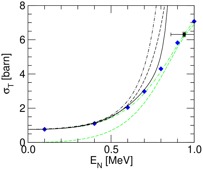
The diamonds are “evaluated data points” from Ref. BNL . In order to have an idea of the error bars from individual experiments we also show data from Ref. data as the black squares. The EFT in leading (LO), subleading (NLO), and subsubleading (NNLO) orders is represented by the dashed, dash-dotted, and solid black lines, respectively. At LO the scattering length and effective range in the $p_{3/2}$ partial wave as well as the scattering length in the $s_{1/2}$ partial wave contribute. The data are reproduced up to neutron energies of about $E_{N}=0.5$ MeV. Interestingly, the NLO result, which contains only the leading unitarity correction to the LO result and adds no new parameters, worsens the description of the data. At NNLO three more parameters enter: the shape parameter in the $p_{3/2}$ wave, the effective range in the $s_{1/2}$ wave, and the scattering length in the $p_{1/2}$ wave. The data are described up to $E_{N}\approx 0.8$ MeV at NNLO. As expected, the EFT describes the data qualitatively, but it fails in the immediate neighborhood of the resonance. In order to improve the description in this neighborhood, we need to resum the interaction that gives rise to the resonance width. The calculation then has to be organized in accord to Ref. halos . For comparison, we show the first two orders of the resummed EFT as the grey dashed (LO) and dash-dotted (NLO) lines halos . The improvement around the resonance is evident. Because the scales $M_{lo}$ and $M_{hi}$ are not very well separated, that is, $M_{lo}/M_{hi}$ is not very small, the region of improvement is relatively large. The resummation is useful throughout the low-energy region.

In Fig. 3 the results for the differential cross section in the center-of-mass frame are shown as a function of the scattering angle $\theta_{cm}$ at a momentum of $k_{cm}=15.5$ MeV (corresponding to $E_{N}=0.2$ MeV in the $\alpha$ rest frame).

Figure 3: The differential cross section for $n\alpha$ scattering in the center-of-mass frame (in barns/sr) as a function of the scattering angle $\theta_{cm}$ at a momentum of $k_{cm}=15.5$ MeV. The diamonds are evaluated data from Ref. BNL . The dashed, dash-dotted, and solid black lines show the result in the EFT without resummation at LO, NLO, and NNLO, respectively. The grey dashed and dash-dotted lines show the result in the EFT with resummation at LO and NLO, respectively.

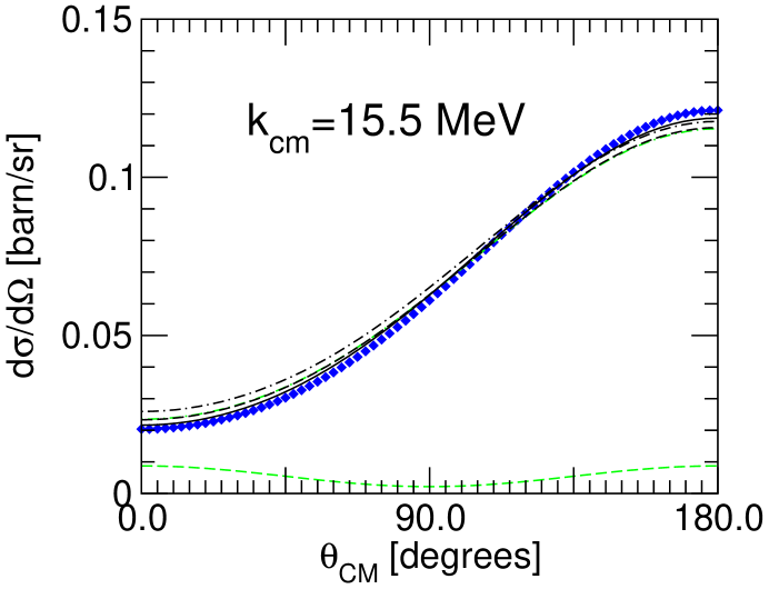
The diamonds are evaluated data from Ref. BNL . The EFT in leading (LO), subleading (NLO), and subsubleading (NNLO) orders is represented by the dashed, dash-dotted, and solid black lines, respectively. The first two orders of the resummed EFT are shown as the grey dashed (LO) and dash-dotted (NLO) lines halos . Both EFTs describe the differential cross section at NLO and higher orders. At LO, however, the resummed EFT badly fails to reproduce the differential cross section, while the EFT without resummation already gives a good description. This is because in the resummed EFT the $s_{1/2}$ wave is suppressed relative to the $p_{3/2}$ wave and does only enter at NLO. In the EFT without resummation, the relative order is changed and both the $s_{1/2}$ and $p_{3/2}$ waves enter at LO.

In summary, we have discussed the treatment of shallow resonances in EFT. Although the unitarization done in Ref. halos is not necessary except near the resonance, it improves the description throughout the low-energy region. We have considered explicitly only the case of identical, spinless, heavy particles, but the same ideas apply to other cases, such as $\pi N$ scattering near the Delta resonance —in this context, see Ref. dandelta — and various low-energy nuclear reactions. We illustrated this statement by a study of $n\alpha$ scattering.

References

- (1) P.F. Bedaque and U. van Kolck, Ann. Rev. Nucl. Part. Sci. 52, 339 (2002); S.R. Beane, P.F. Bedaque, W.C. Haxton, D.R. Phillips, and M.J. Savage, in Boris Ioffe Festschrift, ed. M. Shifman (World Scientific, Singapore, 2001).
- (2) Nuclear Physics with Effective Field Theory II, ed. P.F. Bedaque, M.J. Savage, R. Seki, and U. van Kolck (World Scientific, Singapore, 1999); Nuclear Physics with Effective Field Theory, ed. R. Seki, U. van Kolck, and M.J. Savage (World Scientific, Singapore, 1998).
- (3) C.A. Bertulani, H.-W. Hammer, and U. van Kolck, Nucl. Phys. A 712, 37 (2002).
- (4) D.R. Tilley, H.R. Weller, and G.M. Hale, Nucl. Phys. A 541, 1 (1992).
- (5) N. Tanaka, Y. Suzuki, K. Varga, and R.G. Lovas, Phys. Rev. C 59, 1391 (1999).
- (6) D.B. Kaplan, Nucl. Phys. B 494, 471 (1997).
- (7) U. van Kolck, hep-ph/9711222, in Proceedings of the Workshop on Chiral Dynamics 1997, Theory and Experiment, ed. A. Bernstein, D. Drechsel, and T. Walcher (Springer-Verlag, Berlin, 1998); Nucl. Phys. A 645, 273 (1999).
- (8) B. Gelman and U. van Kolck, in progress.
- (9) R.A. Arndt, D.L. Long, and L.D. Roper, Nucl. Phys. A 209, 429 (1973).
- (10) Evaluated Nuclear Data Files, National Nuclear Data Center, Brookhaven National Laboratory ( http://www.nndc.bnl.gov/ ).
- (11) B. Haesner et al., Phys. Rev. C 28, 995 (1983); M.E. Battat et al., Nucl. Phys. 12, 291 (1959).
- (12) V. Pascalutsa and D.R. Phillips, nucl-th/0212024.