Nuclear level statistics: extending the shell model theory to higher temperatures

Abstract

The Shell Model Monte Carlo (SMMC) approach has been applied to calculate level densities and partition functions to temperatures up to $\sim 1.5-2$ MeV, with the maximal temperature limited by the size of the configuration space. Here we develop an extension of the theory that can be used to higher temperatures, taking into account the large configuration space that is needed. We first examine the configuration space limitation using an independent-particle model that includes both bound states and the continuum. The larger configuration space is then combined with the SMMC under the assumption that the effects on the partition function are factorizable. The method is demonstrated for nuclei in the iron region, extending the calculated partition functions and level densities up to $T\sim 4$ MeV. We find that the back-shifted Bethe formula has a much larger range of validity than was suspected from previous theory. The present theory also shows more clearly the effects of the pairing phase transition on the heat capacity.

I Introduction

Consistent calculations of nuclear partition functions and level densities are required in nuclear astrophysics. The nuclear partition functions at a finite temperature are needed to understand pre-supernova collapse bethe79 and for the calculation of stellar thermal reaction rates rauscher00 . Similarly, level densities determine the statistical neutron and proton capture cross-sections in nucleosynthesis bbfh57 .

The Fermi gas formula (also known as the Bethe formula) bethe36 for the nuclear level density can be derived from the partition function of non-interacting nucleons bm69 . Correlation effects, e.g., shell, pairing and deformation effects, are usually accounted for through empirical modifications of this formula. In particular, the back-shifted Bethe formula gc65 ; hm72 is found to describe well the experimental data if its parameters, the single-particle level density parameter $a$ and back-shift parameter $\Delta$, are fitted for each nucleus dilg73 ; il92 . However, these phenomenological approaches cannot be reliably used in nuclei for which experimental data are not available, so there is a need for microscopic theories that include interaction effects. In mean field theory, pairing can be treated in the BCS approximation, as was done in Ref. go96 . However, shape fluctuations are likely to be significant and they require a theory beyond the mean field, e.g., the static path approximation la88 . A theory that includes quadrupole fluctuations in the static path approximation was proposed in Ref. ag98 . Like the mean field theory, the static path approximation allows calculations in large spaces. This was exploited by the authors of Ref. ag98 who presented results for large single-particle spaces including an approximate treatment of unbound states. However, as implemented there, the theory includes neither pairing correlations, which are certainly of similar importance, nor multipoles of the interaction beyond quadrupole.

A more systematic approach to calculate correlation effects is to use the interacting shell model. In this approach, we define a many-particle configuration space and treat in full the effective interaction within that space. Here the shell model Monte Carlo (SMMC) method has rather favorable computational properties, scaling with the number $N$ of single-particle orbitals as $N^{4}$, compared to direct diagonalization methods, which scale exponentially. Even so, most applications of the SMMC have so far been limited to a single major shell. For medium mass nuclei, this restricts the reliability of the calculated partition functions (and associated level densities) to temperatures below $\sim 1.5-2$ MeV na97 ; al99 ; al00 .

In this work, we will first explore the model space truncations in an independent-particle approximation, extending the single-particle space to include both the bound states and the continuum. This was studied within a semiclassical approximation in Ref. tu79 . We will develop the fully quantum-mechanical theory that includes the continuum in Section II. We find that in tightly bound nuclei, the continuum contribution is negligible even at high temperatures (e.g., $T\sim 4$ MeV for ⁵⁶Fe), while in weakly bound nuclei the continuum contribution can become significant already at low temperatures. In either case the continuum contribution can be well approximated by considering just the contribution of the narrow resonances, treated as broadened bound states.

The remaining task is to include interaction effects, as discussed in Section III. It is necessary to distinguish between the long-range part of the interaction, acting in the valence orbitals, and the short-range part, involving highly excited configurations. The short-range part is beyond the scope of the theory, and must be taken into account in defining an effective long-range interaction, but the latter can be accurately treated within the SMMC approach. At higher temperatures, long-range interaction effects are weak and corrections to the entropy from the larger model space can be included in a single-particle approach. We shall see that at high temperatures, the interaction effects on the partition function scale as $1/T$, and the two temperature regimes can be joined smoothly. We find that the extended partition function and its associated level density are well described by the back-shifted Bethe formula up to $T\sim 4$ MeV. This value represents an upper limit for our underlying assumption that the single-particle potential is fixed and independent of temperature.

The basic object we study is the canonical partition function defined by

$$Z(\beta)={\rm Tr}e^{-\beta H}\;,$$ (1)

where $\beta$ is the inverse temperature, $\beta=1/T$, and the trace is taken at a fixed particle number (i.e., fixed number of protons and neutrons). We shall find it convenient to measure the energy with respect to the ground energy $E_{0}$, defining an excitation partition function $Z^{\prime}$ as

$$Z^{\prime}\equiv Ze^{\beta E_{0}}\;.$$ (2)

Thus at zero temperature, the excitation partition function is equal to the degeneracy of the ground state $N_{\rm gs}$, $Z^{\prime}(T=0)=N_{\rm gs}$.

The conversion from the partition function to the level density is discussed in Section IV. While the results of the theory can be given as numerical tables of $Z(T)$ and the corresponding level density $\rho(E)$, it is also useful to express the results in terms of the parameters of the back-shifted Bethe formula, which provides a good description at not too low temperatures. The inclusion of a back shift requires a particular parameterization of $Z^{\prime}$, as discussed in Section III.

II Orbital truncation effects in the independent-particle approximation

When the temperature is larger than about a third of the nucleon separation energy, the unbound nucleon states can no longer be ignored. To develop a theory that includes the continuum, we first need to define precisely how we separate the contributions of the free nucleons and the nucleus to the partition function. If the system is enclosed in a box, the free nucleon partition function is proportional to the volume of this box. The contribution of the continuum to the nuclear partition function is found by the explicit subtraction of the free-particle contribution, and is independent of the volume of the box, if it is large compared to the size of the nucleus. The free nucleon partition function we use here is the one obtained when the nuclei are ignored entirely.

In the independent-particle approximation, the single-particle spectrum is calculated in an external potential well, representing the nuclear mean-field potential. Assuming the well to be spherically symmetric, the bound state energies $\epsilon_{nlj}$ depend only on the principal quantum number $n$, orbital angular momentum $l$, and total spin $j$. For the positive energy continuum, we need the scattering phase shifts $\delta_{lj}(\epsilon)$ where $\epsilon$ is the (positive) energy of the continuum states. The change $\delta\rho$ in the single-particle continuum level density in the presence of the potential $V$ is found by subtracting the free particle level density $\rho_{0}$ from the total density $\rho$:

$$\delta\rho(\epsilon)=\rho(\epsilon)-\rho_{0}(\epsilon)=\sum_{lj}(2j+1){1\over\pi}{d\delta_{lj}\over d\epsilon}\;.$$ (3)

We denote the many-body grand canonical partition function in the independent-particle approximation by $Z^{\rm GC}_{\rm sp}$, where the subscript stands for “single-particle.” It is given by

$$\ln Z^{GC}_{sp}(\beta,\mu)=\sum_{nlj}(2j+1)\ln[1+e^{-\beta(\epsilon_{nlj}-\mu)}]+\int_{0}^{\infty}d\epsilon\delta\rho(\epsilon)\ln[1+e^{-\beta(\epsilon-\mu)}]\;,$$ (4)

where $\mu$ is the chemical potential. A more convenient form, avoiding the phase-shift derivative, may be obtained by integrating the second term in the above equation by parts. The contribution from the integral endpoint at $\epsilon=0$ is evaluated using Levinson’s theorem, $\delta_{lj}(\epsilon=0)=n_{lj}\pi$, where $n_{lj}$ is the number of bound $lj$ states. The result is

$$\int_{0}^{\infty}d\epsilon{d\delta_{lj}\over d\epsilon}\ln[1+e^{-\beta(\epsilon-\mu)}]=-n_{lj}\pi\ln(1+e^{\beta\mu})+\beta\int_{0}^{\infty}d\epsilon\;\delta_{lj}(\epsilon)f(\epsilon)\;,$$ (5)

where $f(\epsilon)=[1+e^{\beta(\epsilon-\mu)}]^{-1}$ is the Fermi-Dirac occupation. The formula for the partition function can then be rewritten

$$\ln Z^{\rm GC}_{sp}(\beta,\mu)=\sum_{lj}(2j+1)\left\{\sum_{n}\ln\left[{1+e^{-\beta(\epsilon_{nlj}-\mu)}\over 1+e^{\beta\mu}}\right]+{\beta\over\pi}\int_{0}^{\infty}d\epsilon\;\delta_{lj}(\epsilon)f(\epsilon)\right\}\;.$$ (6)

This form is easier to use computationally because it avoids numerical derivatives.

To calculate the partition function of a specific nucleus, we need to transform the grand canonical partition to the canonical partition function at fixed proton and neutron numbers. In the saddle point approximation, the corresponding correction is estimated from the particle-number fluctuations in the grand-canonical ensemble, giving for the canonical $Z(\beta)$

$$Z(\beta)\approx\left(2\pi\langle(\Delta N)^{2}\rangle\right)^{-1/2}Z^{\rm GC}\;e^{-\beta\mu N}\;,$$ (7)

or

$$\ln Z^{\prime}\approx\ln Z^{\rm GC}+\beta E_{0}-\beta\mu N-{1\over 2}\ln\left(2\pi\langle(\Delta N)^{2}\rangle\right)\;.$$ (8)

Here $\langle(\Delta N)^{2}\rangle$ is the variance of the neutron or proton number and $Z^{\prime}=Ze^{\beta E_{0}}$. In Eq. (8), $\mu$ is calculated from $\langle\hat{N}\rangle=\partial\ln Z^{\rm GC}/\partial\alpha=N$ (where $\langle\hat{N}\rangle$ is the average particle number in the grand-canonical ensemble and $\alpha=\beta\mu$), and the variance is found from $\langle(\Delta N)^{2}\rangle={\partial^{2}\ln Z^{\rm GC}/\partial\alpha^{2}}$. In the independent-particle approximation these quantities are

$$N={\partial\ln Z^{\rm GC}_{\rm sp}\over\partial\alpha}=\sum_{lj}(2j+1)\left[\sum_{n}f_{nlj}+{1\over\pi}\int_{0}^{\infty}d\epsilon{d\delta_{lj}\over d\epsilon}f(\epsilon)\right]\;,$$ (9)

$$\langle(\Delta N)^{2}\rangle={\partial^{2}\ln Z^{\rm GC}_{\rm sp}\over\partial\alpha^{2}}=\sum_{lj}(2j+1)\left[\sum_{n}f_{nlj}(1-f_{nlj})+{1\over\pi}\int_{0}^{\infty}d\epsilon{d\delta_{lj}\over d\epsilon}f(1-f)\right]\;.$$ (10)

To avoid numerical derivatives, we can again use integration by parts and rewrite Eqs. (9) and (10) as

$$N=\sum_{lj}(2j+1)\left[\sum_{n}[f_{nlj}-f(0)]+{\beta\over\pi}\int_{0}^{\infty}d\epsilon\;\delta_{lj}(\epsilon)f(1-f)\right]\;,$$ (11)

and

$$\langle(\Delta N)^{2}\rangle=\sum_{lj}(2j+1)\left\{\sum_{n}\left[f_{nlj}(1-f_{nlj})-f(0)(1-f(0))\right]\right.$$

$$\left.+{\beta\over\pi}\int_{0}^{\infty}d\epsilon\;\delta_{lj}(\epsilon)f(1-f)(1-2f)\right\}\;.$$ (12)

To illustrate the method, we apply it to nuclei in the iron region. For the mean-field potential we use a Woods-Saxon well $V(r)$ plus a spin-orbit interaction

$$V(r)+\lambda_{ls}(\ell\cdot{\bf s})r_{0}^{2}{1\over r}{dV\over dr}\;,$$ (13)

where $V(r)=V_{0}\left[1+\exp(r-R_{0})/a\right]^{-1}$ with $R_{0}=r_{0}A^{1/3}$. We choose the parameterization of Ref. bm69 , where $V_{0}=-51+33{N-Z\over A}$ MeV, $a=0.67$ fm, $r_{0}=1.32$ fm, and $\lambda_{\ell s}=-0.44$. We have calculated the single-particle spectrum and scattering phase shifts in this potential well, and used them to compute the canonical partition function from Eqs. (8), (6) and (II). The solid line in Fig. 1 shows the logarithm of the canonical excitation partition function $\ln Z_{\rm sp}^{\prime}$ for the nucleus ⁵⁶Fe when the full single-particle space (bound states plus continuum) is taken into account.

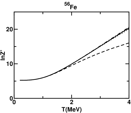
Figure 1: The logarithm of the canonical excitation partition function $Z^{\prime}_{sp}$ (where the energy is measured with respect to the ground-state energy) calculated for ⁵⁶Fe is shown for the following single-particle spaces: all bound states plus continuum as described by Eqs. (6), (8), and (II) (solid line); bound states and the narrow resonances listed in Table I (dashed-dotted line); and bound states only (dotted line). The corresponding calculation with the space truncated to the $fpg$ major shell is shown as the dashed line. The intercept at $T=0$ is $\ln N_{\rm gs}$, where $N_{\rm gs}=168$ is the number of states in the $(f^{p}_{7/2})^{-2}(p^{n}_{3/2})^{2}$ shell configuration.

Table 1: Neutron orbital energies and resonance energies (in MeV) in ⁵⁶Fe, calculated with the Woods-Saxon potential of Ref. bm69 .

Orbital type	$l,j$	$\epsilon$ (56Fe)	$\epsilon$ (66Cr)
bound	$f_{7/2}$	-12.68	-10.2
	$p_{3/2}$	-8.65	-6.7
	$p_{1/2}$	-6.56	-5.1
	$f_{5/2}$	-6.34	-5.2
	$g_{9/2}$	-3.13	-1.7
	$d_{5/2}$	-0.41
	$s_{1/2}$	-0.26
resonance	$d_{5/2}$		0.35
	$g_{7/2}$	4.95	4.67
	$h_{11/2}$	6.22	6.62

We next investigate various truncations within the independent-particle model. Of particular interest is the truncation to the same model space that is used in the SMMC approach. Most of the SMMC calculations so far have been restricted to the bound states in a single major shell. For example calculations in the iron region were restricted to the complete $fpg_{9/2}$ major shell, which includes the active orbitals $f_{7/2},p_{3/2},p_{1/2},f_{5/2}$ and $g_{9/2}$. The orbital energies [determined in a Woods-Saxon well with spin-orbit interaction (13)] are given in Table I.

The partition function calculated in this truncated space (in the independent-particle approximation) is compared with the full space calculation [Eqs. (6), (8) and (II)] in Fig. 1. One sees that the truncation to a single major shell becomes problematic at temperatures above $\sim 1.5$ MeV.

To assess the importance of the continuum, we also show in Fig. 1 the result of the calculation keeping all bound states but neglecting the continuum integral. One sees that the continuum contribution is not very significant for a tightly bound nucleus such as ⁵⁶Fe.

However this situation changes in a nucleus with a small neutron separation energy. In Fig. 2 we compare the calculations in the full single-particle space and in the truncated space that includes all bound states for the nucleus ⁶⁶Cr. Here the separation energy of the highest occupied orbital is 1.7 MeV. One sees that the continuum effects become significant for $T\gtrsim 1$ MeV.

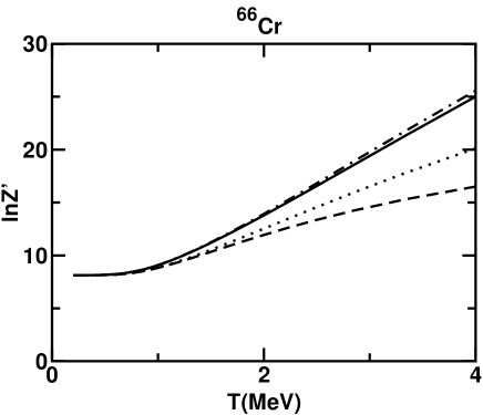
Figure 2: Similar to Fig. 1 but for the nucleus ⁶⁶Cr.

Rather than ignoring the continuum completely, one could also consider the approximation of including only narrow resonances, treating them as broadened discrete states. Indeed, the derivative of the scattering phase shift $\delta_{lj}$ in the vicinity of a narrow resonance follows a Lorentzian

$${d\delta_{lj}\over d\epsilon}\approx{\Gamma^{r}_{lj}/2\over(\epsilon-\epsilon^{r}_{lj})^{2}+(\Gamma^{r}_{lj}/2)^{2}}\;,$$ (14)

where $\epsilon^{r}_{lj}$ and $\Gamma^{r}_{lj}$ are the centroid and width of a resonance with quantum numbers $lj$. If the resonance width $\Gamma^{r}_{lj}$ is much smaller than $T$, the integral in (4) can be evaluated to give a contribution to $\ln Z_{sp}^{GC}$ as though the resonance were a discrete state with energy $\epsilon^{r}_{lj}$.

We identify the resonances from the energy dependence of the phase shifts $\delta_{lj}$ in different channels $lj$, and take their energies where the phase shifts ascend through $\pi/2$. The channels with resonances and their energies are displayed in Table I. The partition function calculated using bound states and narrow resonances is shown as the dotted line in Fig. 2. We see that the resonance approximation is good at least to $T\sim 3.5$ MeV.

We now summarize the validity of the various approximations, requiring that the theory be accurate up to temperatures of $T\sim 4$ MeV. For nuclei along the stability line, it is only necessary to include bound states. If one goes to nuclei that have much lower separation energies, the continuum contribution can be significant but the resonance approximation is likely to be adequate. It should be emphasized throughout this section we have assumed a fixed mean-field potential. Above $T\sim 4$ MeV, that approximation becomes unreliable.

III Interaction effects

We next discuss interaction effects on the partition function. The ground-state binding energy is of course very sensitive to the interaction, but this will not be immediately visible in the excitation partition function. Let us denote by $Z^{\prime}_{v,tr}$ the partition function calculated with interactions but in a truncated single-particle space. We argue that the correction due to a larger model space will be largely additive in the logarithm of the partition function, so that the way to combine a small-space calculation of interaction effects with a large-space calculation of the independent-particle partition $Z^{\prime}_{sp}$ is with the formula

$$\ln Z^{\prime}_{v}=\ln Z^{\prime}_{v,tr}+\ln Z^{\prime}_{sp}-\ln Z^{\prime}_{sp,tr}\;,$$ (15)

where $Z^{\prime}_{sp,tr}$ is the excitation partition function (in the absence of interactions) in the same truncated single-particle space in which $Z^{\prime}_{v,tr}$ is calculated.

Eq. (15) cannot be justified rigorously, but we can motivate it in several ways. It is certainly true that the interaction corrections approach zero at high temperature. From finite-temperature many-body perturbation theory, it is seen that the leading corrections to the independent-particle Hamiltonian $H_{0}$ are additive in the logarithm of the partition function, as is assumed in Eq. (15). The explicit formula is

$$\ln{\rm Tr}\ \exp(-\beta K)-\ln{\rm Tr}\ \exp(-\beta K_{0})=-\int_{0}^{\beta}d\tau\langle V_{I}(\tau)\rangle+\frac{1}{2}\int_{0}^{\beta}d\tau_{1}\int_{0}^{\beta}d\tau_{2}\langle T_{\tau}V_{I}(\tau_{1})V_{I}(\tau_{2})\rangle_{\rm conn}+\ldots\;,$$ (16)

where $K=H-\mu\hat{N}$, $K_{0}=H_{0}-\mu\hat{N}$, $V_{I}$ is the two-body interaction in the interaction picture (with respect to $K_{0}$), $T_{\tau}$ denotes time ordering and $\langle\ldots\rangle$ denotes a thermal average with respect to $K_{0}$. Each integration in (16) gives a factor $1/T$. In cases where analytic expressions can be derived (e.g., hard core gas and Coulomb gas), it may be verified that the interaction correction falls off as $T^{-1}$ or more strongly at high $T$. At low temperatures, the extended space is not thermally occupied and only plays an indirect role, renormalizing the interactions in the smaller space. Since the SMMC is applied with renormalized interactions that are appropriate for the smaller space, there is no additional correction when the larger space is considered explicitly. With the correct limiting behavior at both low and high temperatures, we have a better theory for the complete temperature dependence.

We now give a brief summary of the SMMC calculations to be used for $Z^{\prime}_{v,tr}$ in Eq. (15). The interaction is taken to be the same as in Ref. na97 . It is separable and surface-peaked, acting between orbitals of a major shell (here the $fpg_{9/2}$ orbitals). The strength of the surface-peaked interaction is determined self-consistently and renormalized appropriately for each multipole. In addition, there is a monopole pairing interaction, whose strength is determined from odd-even mass differences. The single-particle Hamiltonian is the same as in Section II. The outputs of the SMMC computation are canonical expectation values of various observables. For our purposes here, the most important quantity is the canonical thermal energy $E(\beta)$, calculated as the expectation of the Hamiltonian with number-projected SMMC densities. The partition function is then found by integration

$$\ln Z(\beta)=\ln Z(0)-\int_{0}^{\beta}d\beta^{\prime}E(\beta^{\prime})\;.$$ (17)

Here $Z(0)$ is the partition function at $T\to\infty$ and is equal to the total number of many-particle states in the model space. In addition, we need to determine the ground-state energy $E_{0}$ in order to find the excitation partition function, Eq. (2). This is done by extrapolating the calculated $E(\beta)$ to large $\beta$.

Figure 3: The excitation partition function of ⁵⁶Fe using the SMMC method in the truncated space ($fpg_{9/2}$). The partition function $Z^{\prime}_{v,tr}$ in the presence of the residual interaction (squares) is compared to the SMMC partition function $Z^{\prime}_{sp,tr}$ in the absence of interactions (circles). The dashed line is the partition function of the independent-particle model calculated in the saddle point approximation using Eqs. (8), (6) and (II).

The SMMC results for the nucleus ⁵⁶Fe are shown in Fig. 3, with $\ln Z^{\prime}_{v,tr}$ plotted as a function of $T$ (squares). The curve starts out flat, changing to a linear increase over some range of $T$, and reaching a plateau beyond the highest temperature plotted. The initial flat behavior is associated with the gap in the energy spectrum between the ground state and the first excited state, while the linear regime corresponds to the Bethe formula. The saturation is due to the truncation of the space, and its onset marks the limit of validity of the truncated SMMC calculation. We next repeat the SMMC calculation with the two-body interaction turned off. The results are shown by the circles in Fig. 3. Notice that the difference between the two partition functions becomes small as the temperature increases, confirming the analysis in an earlier part of this section [see in particular Eq. (16)].

Before calculating the partition function in the extended model space, we also compare in Fig. 3 two ways of calculating the non-interacting partition function, from Eq. (8) (dashed line) or from the SMMC with the interaction turned off (squares). In the latter method, particle-number projection is carried out exactly, while in Eq. (8) this is done in the saddle point approximation. One can see that the differences are insignificant for our purposes.

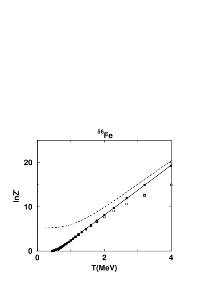
Figure 4: Extended partition function for ⁵⁶Fe, calculated from Eq. (15) shown as solid squares. The solid line is a fit to Eq. (19) with $a=5.87$ MeV^-1 and $\Delta=1.03$ MeV. Shown for comparison are the SMMC (open squares) and the full space single-particle (dashed line) results.

We now combine the various terms in Eq. (15) to get our extended-range partition function. The result is shown in Fig. 4 by the solid squares. For comparison, the SMMC result (open squares) and the full space independent-particle model result (dashed line) are shown as well. Remarkably, the extended $\ln Z^{\prime}$ is seen to be close to a linear function of $T$ over most of the range, unlike either of its constituents. In the saddle point approximation, the dominating term in $\ln Z^{\prime}$ is linear in $T$ with whose slope is the parameter $a$ in the level density formula. However, to compare with the back-shifted Bethe formula [see Eq. (27) in Section IV], more care is needed in treating the sublinear terms. Starting from the Darwin-Fowler expression for the partition function of non-interacting fermions [see Eq. (2B-9) in Ref. bm69 ], and including the proton and neutron number fluctuation terms from Eq. (8), one can derive the following expression for $Z^{\prime}$,

$$\ln Z^{\prime}\approx aT-\ln(6aT/\pi)\;,$$ (18)

where $a=\pi^{2}g/3$ and g is either the proton or neutron single-particle level density at the Fermi energy (assumed to be equal). Within the saddle-point approximation, Eq. (18) is equivalent to the simple Bethe formula for the level density (see Section IV). As mentioned in the introduction, a better phenomenological description of the measured level density is often obtained by shifting the ground state energy by an amount $\Delta$ in the Bethe formula. We show in Appendix A that the corresponding modification of the partition function is to introduce a third term in Eq. (18),

$$\ln Z^{\prime}\approx aT-\ln(6aT/\pi)-\Delta/T\;.$$ (19)

The solid line in Fig. 4 is a fit of (19) to $\ln Z^{\prime}$ for $1\lesssim T\lesssim 4$ MeV with $a=5.87$ MeV^-1 (corresponding to the expression $a=A/K$ with $K=9.5$ MeV) and $\Delta=1.03$ MeV. The fit does remarkably well in describing the $T$-dependence of $\ln Z^{\prime}$ for temperatures between $T\sim 1$ MeV and $T\sim 4$ MeV (the rms of the deviation from the calculated $\ln Z^{\prime}$ is $0.05$). The functional form (19) of $\ln Z^{\prime}$ is the essence of the (back-shifted) Bethe level density formula; the result observed here implies that this formula is useful to considerably higher temperatures than was apparent in earlier calculations. At high temperatures, the dominant term in (19) is linear in $T$. However, the other two terms are necessary to obtain a value of $a$ that is comparable to the value extracted directly from the level density, which will be the subject of Section IV.

In the independent-particle model, $\ln Z^{\prime}$ is approximately linear in $T$ only for $T\gtrsim 2$ MeV with a slope of $a\approx 5.25$ MeV^-1, i.e., $K\approx 10.7$. This value of $K$ is smaller than the Fermi gas value bm69 $K\approx 15$ but still larger than the value we found above when correlations are taken into account.

The canonical entropy can be calculated from $S=-\partial F/\partial T$ where $F=-T\ln Z^{\prime}$ is the canonical free energy. Using the empirical formula (19), this entropy is given by

$$S\approx 2aT-\ln(6aT/\pi)-1\;,$$ (20)

and is independent of the back-shift parameter $\Delta$. Thus the parameter $a$ can be determined by a single parameter fit of the extended entropy to (20). The leading order term in the entropy is linear in $T$ and the last two terms in (20) originate in the particle number fluctuations. The microscopic calculation of the extended entropy can be done without taking numerical derivate with respect to $T$, as is explained in Section IV. Fig. 5 shows a fit of the empirical formula (20) (solid line) to the extended entropy in the range $T\sim 1-4$ MeV (symbols) with $a=5.82$ MeV^-1 (the rms deviation is $\approx 0.3$). This value of $a$ is in agreement with the value found from $\ln Z^{\prime}$. The fit is good and only at $T\sim 4$ MeV, do we start to observe a small deviation.

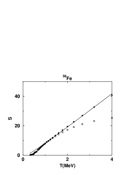
Figure 5: The extended entropy of ⁵⁶Fe (solid squares). The solid line is a fit to Eq. (20) with $a=5.82$ MeV^-1. The open squares describe the SMMC entropy.

Figure 6: The extended partition function (solid squares) for the odd-even nucleus ⁵⁷Fe is compared with the SMMC partition function (open squares). The solid line is a fit to the back-shift formula (19) with $a=6.04$ MeV^-1 and $\Delta=-1.29$ MeV.

We have demonstrated our method for an even-even nucleus ⁵⁶Fe, but it should be equally applicable to odd-even and odd-odd nuclei. As an example we show in Fig. 6 the logarithm of the excitation partition function for ⁵⁷Fe. The solid line is a fit to (19) with $a=6.04$ MeV^-1 and $\Delta=-1.29$ MeV in the range $1\lesssim T\lesssim 4$ MeV (the rms deviation is $\approx 0.08$). A qualitative difference is that unlike the case of ⁵⁶Fe, $\ln Z^{\prime}$ does not approach zero at low temperatures. This is due to the spin degeneracy of the ground state of an even-odd nucleus and the much smaller energy gap to the first excited state.

IV Level densities

We now determine the level densities associated with the extended partition function of the previous section. The level densities are calculated from the partition function as in Refs. na97 and al99 using the saddle-point formula

$$\rho(E)=(2\pi\beta^{-2}C)^{-1/2}e^{S}\;,$$ (21)

where $S=\ln Z+\beta E=\ln Z^{\prime}+\beta(E-E_{0})$ is the canonical entropy and $C=-\beta^{-2}dE/d\beta$ is the canonical heat capacity. The thermal energy in (21) is a function of $\beta$ determined by

$$E-E_{0}=-{\partial\ln Z^{\prime}\over\partial\beta}\;.$$ (22)

Using the expression (15) for the extended partition function and Eq. (22), we have

$$E-E_{0}=(E_{v,tr}-E^{0}_{v,tr})+[E_{sp}-(E_{sp,tr}+E_{\rm core}^{0})]\;,$$ (23)

where $E_{\rm core}^{0}=E_{sp}^{0}-E_{sp,tr}^{0}$ is the $T=0$ energy of the core (i.e., the shells below the valence shell). The notation used here for the various energies follows the same notation used for the partition functions in (15) and the subscript or superscript “0” denotes the ground state in the corresponding model space.

Similarly, we find for the extended entropy and heat capacity

$$S = S_{v,tr}+S_{sp}-S_{sp,tr}$$

$$C = C_{v,tr}+C_{sp}-C_{sp,tr}\;.$$ (24)

Eq. (23) is used to determine the relation between the excitation energy and $\beta$ in the calculation of the extended level density. When the SMMC approach is used to calculate interaction effects in the truncated space, $E_{v,tr}$ is calculated directly from the expectation value of the Hamiltonian and $E^{0}_{v,tr}$ is found by extrapolation to $\beta\to\infty$. The partition $Z_{v,tr}$ (and therefore the entropy $S_{v,tr}$) is found by integration using (17), while the heat capacity $C_{v,tr}$ is found by a numerical derivative of the energy.

It remains to determine the respective quantities in the independent-particle model (both in the full and truncated spaces). Here there is a technical complication in that the needed quantities are canonical. For example, we need to calculate the canonical energies $E_{sp}$ and $E_{sp,tr}$. In principle, one can use (22) where $Z$ is calculated in the independent-particle model. However, since $Z$ is a canonical partition function, the partial derivative with respect to $\beta$ must be evaluated at constant particle number $N$ rather than at constant $\alpha$ ($\alpha=\beta\mu$). The explicit expressions for $E_{\rm sp}$ and $C_{\rm sp}$ in terms of logarithmic derivatives of the grand-canonical partition function are derived in Appendix B. In Appendix C we express these logarithmic derivatives in terms of the corresponding single-particle spectrum and scattering phase shifts.

Figure 7: Level density of ⁵⁶Fe, calculated with the extended partition function (solid squares). The solid line is a fit to the back-shifted Bethe formula (27) and describes well the extended level density in the full excitation energy range shown in the figure. The SMMC level density in the truncated $fpg_{9/2}$ shell is shown by open squares and the independent-particle model level density is shown by the dashed line.

The extended level density of ⁵⁶Fe is shown in Fig. 7 (solid squares) as a function of excitation energy, $E_{x}=E-E_{0}$. For comparison, the SMMC level density calculated in the truncated space (i.e., $fpg_{9/2}$ shell) is shown by open squares, while the level density calculated in the independent-particle model (no truncation) is shown by the dashed line.

To derive the back-shifted Bethe formula for the level density, we evaluate the inverse Laplace transform of $Z^{\prime}$ in Eq. (18) in the saddle point approximation (separating out the particle number fluctuation term as a pre-exponential factor). We find

$$\rho\approx(2\pi)^{-1/2}\left(-{\partial E\over\partial\beta}\right)^{-1/2}\left({\pi\over 6aT}\right)e^{aT-\Delta/T+\beta(E-E_{0})}={\sqrt{\pi}\over 12}a^{-3/2}T^{-5/2}e^{2aT}\;,$$ (25)

where the temperature is determined by the excitation energy $E_{x}=E-E_{0}$ through

$$E_{x}\approx aT^{2}+\Delta\;.$$ (26)

Relation (26) generalizes the usual Bethe relation $E_{x}=aT^{2}$ to include an empirical offset $\Delta$ to the ground-state energy. This offset originates in correlation effects.

When expressed in terms of the excitation energy, Eq. (25) is just the back-shifted Bethe formula

$$\rho(E_{x})={\sqrt{\pi}\over 12}a^{-1/4}(E_{x}-\Delta)^{-5/4}\exp[2\sqrt{a(E_{x}-\Delta)}]\;.$$ (27)

This formula has two fit parameters, the single-particle level density parameter $a$ and the back-shift parameter $\Delta$. Fitting (27) to the calculated extended level density in the range $5\lesssim E_{x}\lesssim 60$ MeV, we find $a=5.9$ MeV^-1 and $\Delta=1.35$ MeV (with a $\chi^{2}$ per degree of freedom below 1), in overall agreement with the values found in Section III by fitting (19) to $\ln Z^{\prime}$. These values of $a$ and $\Delta$ are also in close agreement with the earlier values found by fitting to the SMMC level density in the energy range $5\lesssim E_{x}\lesssim 16$ MeV, $a=5.85$ MeV^-1 and $\Delta=1.37$ MeV. However, now the back-shifted Bethe formula (27) describes the extended level density up to much higher values of $E_{x}$ ($\sim 90$ MeV). Thus the validity of this formula is now extended to significantly higher excitation energies than previously thought. Furthermore, the specific values of the parameters $a$ and $\Delta$ found in previous SMMC calculations al99 are approximately valid in this extended energy range.

Figure 8: Extended level density (solid squares) in comparison with the SMMC level density (open squares) for ⁵⁷Fe. The solid line is a fit to the back-shifted Bethe formula (27).

Fig. 8 shows the level density of the odd-$A$ nucleus ⁵⁷Fe, where we find in the extended range $a=6.05$ MeV^-1 and $\Delta=-1.3$ MeV. These values are comparable to the values determined from $\ln Z^{\prime}$ in Section III.

The good fits we find to the back-shifted formulas (19) and (27), for the logarithm of the partition function and the level density, respectively, imply that the excitation energy can be approximated by the quadratic expression (26) for not too low temperatures.

Experimentally, the statistical properties of nuclei at higher temperatures have been deduced from heavy ion reactions. If the nuclei are equilibrated when they decay, there is a direct relation between the kinetic energy distributions of the decay products and the temperature of the daughter nucleus. Experimental results have been reported indicating that the quadratic dependence of $E_{x}$ on temperature needed to be modified at high temperature go89 . However in other experiments only a slight deviation was found ca00 . These latter experiments concluded a weak decrease of $a$ with temperature and even a constant $a$ could not be excluded, in agreement with our results.

V Heat capacity and the pairing phase transition

The back-shifted parameterization works well for temperatures $T\gtrsim 1$ MeV, but not at lower temperatures. The deviations can be clearly seen in the canonical heat capacity as a function of the temperature. There can be a peak in this function that is associated with the pairing phase transition, but the back-shifted parameterization permits only a monotonic function rising linearly with temperature. Recently, experiments in rare-earth nuclei have been reported in which effects of pair breaking can be seen in the canonical heat capacity me99 ; sc01 . The authors measured the level density, constructed a canonical partition function from their data, and used it to deduce the heat capacity as a function of temperature.

Such low temperature characteristics, especially those requiring numerical derivatives, are nontrivial to calculate in the SMMC, but in Ref. li01 a method was found to accurately calculate the heat capacity in the temperature range of interest. A slight enhancement over the Fermi gas heat capacity was found in even iron nuclei around $T\sim 0.8$ MeV. This enhancement is more pronounced for the neutron-rich iron isotopes and is correlated with the reduction in the number of $J=0$ neutron pairs with temperature. However, because the calculation was restricted to a finite space ($fpg_{9/2}$ shell), the calculated heat capacity reached a maximum around temperatures of $\sim 1.5$ MeV and the effect of the pairing phase transition was less pronounced.

Figure 9: The extended heat capacity of ⁵⁶Fe versus temperature, showing a bump around the pairing transition temperature (solid squares). The SMMC heat capacity is shown by the open squares. The dashed line is the heat capacity obtained from the independent-particle model (bound states plus continuum).

Here we use the extended theory to display the heat capacity in a much broader temperature range (i.e., up to $\sim 4$ MeV), where deviations from the basic linear dependence become obvious. The effect of the pairing transition on the heat capacity is now clearly observed even in the iron isotopes with a smaller number of neutrons in which the effect was not noticeable before, e.g., ⁵⁶Fe. Fig. 9 shows the extended heat capacity of ⁵⁶Fe calculated from (IV) and (34) (solid squares) in comparison with the independent-particle heat capacity calculated in the full space (solid line). Contrary to the SMMC heat capacity, the extended heat capacity continued to increase monotonically with temperature as does $C_{sp}$. However, it also exhibits a ‘shoulder’ at low temperatures that is a clear signature of the pairing phase transition and is qualitatively similar to the measured heat capacity in even-even rare-earth nuclei sc01 .

VI Conclusion

In this work we have combined the partition function of the independent-particle model in the full space with the partition function of the interacting shell model calculated in a small space by the SMMC method. This enables us to extend the SMMC calculations of partition functions and level densities up to significantly higher temperatures. The results for iron nuclei suggest that the back-shifted Bethe formula (27) (with temperature-independent parameters) is valid over a wide range of temperatures extending from $T\sim 1$ MeV to $T\sim 4$ MeV. The two parameters of the formula, the single-particle level density parameter $a$ and the back shift $\Delta$, agree well with the empirical values. A corresponding empirical formula (19) that accommodates correlation effects describes well the logarithm of the excitation partition function.

Expressed in the form $a=A/K$, the theoretical value for ⁵⁶Fe is $K=9.5$ MeV. This is considerably smaller than the Fermi-gas value of $K\approx 15$ MeV. It is also smaller than the value $K\approx 10.7$ MeV extracted from the high temperature slope of the logarithm of the independent-particle partition function, indicating the importance of correlation effects. In the literature, effective values of the parameter $a$ are often defined from relations that are valid in the Fermi gas limit (and that ignore corrections due to particle-number fluctuations); e.g., $E_{x}=aT^{2}$, $S=2aT$ and $S^{2}=4aE_{x}^{2}$. In the presence of shell and correlation effects, these effective values of $a$ usually differ from each other and exhibit a temperature dependence even at lower temperatures. Using the empirical relation (19) for the partition function, we find a constant value of $a$ that is similar to the value extracted from the level density itself.

The effects of interactions and unbound states were also taken into account in Ref. ag98 . The authors parameterized their results with a temperature-dependent $K$, and found it to vary significantly, unlike our $K$. However, their work only included part of the interaction, omitting in particular the pairing interaction (which is largely responsible for the back shift), and their treatment of the continuum was approximate. The variation they observe at low temperatures $T\sim 1-2$ MeV is at least partly due to definitions of $K$ that are based on the Fermi gas limit.

For temperatures below $\sim 1$ MeV, the pairing effects are strong and beyond the range of applicability of simple parameterizations. This can be seen in the canonical heat capacity if it is displayed over a large temperature range, as we did using our extended theory.

appendix A

In this Appendix we derive the empirical back-shifted formula (19) for the excitation partition function. The partition function is obtained from the level density by a Laplace transform

$$Z^{\prime}(\beta)=\int_{0}^{\infty}\rho(E_{x})e^{-\beta E_{x}}dE_{x}\;.$$ (28)

Substituting the back-shifted Bethe formula (27) for $\rho(E_{x})$ in Eq. (28), and defining $x=E_{x}-\Delta$, we have

$$Z^{\prime}={\sqrt{\pi}\over 12}a^{-1/4}e^{-\beta\Delta}\int^{\infty}x^{-5/4}e^{2\sqrt{ax}-\beta x}\;.$$ (29)

We evaluate the integral in (29) in the saddle point approximation. The saddle point is given by $x_{0}=aT^{2}$, and we find

$$Z^{\prime}\approx{\pi\over 6aT}e^{aT-\Delta/T}\;.$$ (30)

appendix B

In this Appendix we obtain explicit expressions for the canonical energy and heat capacity in the independent-particle approximation in terms of logarithmic derivatives of the grand-canonical partition function.

We introduce the following notation for the logarithmic derivatives of the grand-canonical partition function in the independent-particle model

$${\cal Z}_{a,b}\equiv{\displaystyle{\partial^{a+b}\ln Z_{GC}\over\partial\alpha^{a}\partial\beta^{b}}}\;.$$ (31)

Relation (9) determines $\alpha=\alpha(\beta,N)$. Considering $\alpha$ a function of $\beta$ and $N$ in the relation (9), we find from $dN/d\beta=0$

$${d\alpha\over d\beta}=-{{\cal Z}_{1,1}\over{\cal Z}_{2,0}}$$ (32)

We can now use Eqs. (8) and (22) to obtain

$$E_{sp}=-{\cal Z}_{0,1}+{{\cal Z}_{2,1}\over 2{\cal Z}_{2,0}}-{{\cal Z}_{3,0}{\cal Z}_{1,1}\over 2{\cal Z}_{2,0}^{2}}\;.$$ (33)

Similarly, the canonical heat capacity in the independent-particle model is given by

$$C_{sp}=-\beta^{2}\left(-{\cal Z}_{0,2}+{2{\cal Z}_{1,1}^{2}+{\cal Z}_{2,2}\over 2{\cal Z}_{2,0}}-{{\cal Z}_{2,1}^{2}+2{\cal Z}_{3,1}{\cal Z}_{1,1}+{\cal Z}_{3,0}{\cal Z}_{1,2}\over 2{\cal Z}_{2,0}^{2}}+{4{\cal Z}_{3,0}{\cal Z}_{2,1}{\cal Z}_{1,1}+{\cal Z}_{4,0}{\cal Z}_{1,1}^{2}\over 2{\cal Z}_{2,0}^{3}}-{{\cal Z}_{3,0}^{2}{\cal Z}_{1,1}^{2}\over{\cal Z}_{2,0}^{4}}\right)\;.$$ (34)

Eqs. (33) and (34) are used to calculate the canonical thermal energies and heat capacities in the independent-particle model in both the full and truncated spaces.

appendix C

In this Appendix we derive explicit expressions for the partial derivatives ${\cal Z}_{a,b}$ of the grand-canonical partition function (see Appendix B) in terms of the single-particle spectrum and scattering phase-shifts.

Using Eq. (4), we find

$${\displaystyle{\cal Z}_{a,b}=\sum_{lj}(2j+1)\left[\sum_{n}(-\epsilon_{nlj})^{b}g_{a+b}(\alpha-\beta\epsilon_{nlj})+{1\over\pi}\int_{0}^{\infty}d\epsilon{d\delta_{lj}\over d\epsilon}(-\epsilon)^{b}g_{a+b}(\alpha-\beta\epsilon)\right]\;,}$$ (35)

where we have defined

$$g(x)=\ln(1+e^{x})\;;\;\;\;g_{a}\equiv{d^{a}g\over dx^{a}}\;.$$ (36)

Note that $g_{1}(x)=1/(1+e^{x})=f$, where $f$ is the Fermi-Dirac occupation number for $x=\alpha-\beta\epsilon$. We also have

$$\begin{array}[]{ll}g_{2}=f_{1}=f(1-f)\\ g_{3}=f_{2}=f(1-f)(1-2f)\\ g_{4}=f_{3}=f(1-f)(1-6f+6f^{2})\\ g_{5}=f_{4}=f(1-f)(1-14f+36f^{2}-24f^{3})\end{array}$$ (41)

To avoid the numerical derivative of the phase-shift, we can integrate (35) by parts to obtain

$$\begin{array}[]{ll}{\displaystyle{\cal Z}_{a,b}=}&{\displaystyle(-1)^{b}\sum_{lj}(2j+1)\left\{\sum_{n}\epsilon_{nlj}^{b}g_{a+b}(\alpha-\beta\epsilon_{nlj})-{b\over\pi}\int_{0}^{\infty}d\epsilon\;\delta_{lj}(\epsilon)\epsilon^{b-1}g_{a+b}(\alpha-\beta\epsilon)\right.}\\ &{\displaystyle\left.\;\;\;\;\;\;\;\;\;\;\;\;\;\;\;\;\;\;\;\;\;\;\;\;\;\;\;\;\;\;\;\;\;+{\beta\over\pi}\int_{0}^{\infty}d\epsilon\;\delta_{lj}(\epsilon)\epsilon^{b}g_{a+b+1}(\alpha-\beta\epsilon)\right\}}\end{array}$$ (42)

for $b>0$ and

$${\displaystyle{\cal Z}_{a,0}=\sum_{lj}(2j+1)\left\{\sum_{n}\left[g_{a}(\alpha-\beta\epsilon_{nlj})-g_{a}(\alpha)\right]+{\beta\over\pi}\int_{0}^{\infty}d\epsilon\;\delta_{lj}(\epsilon)g_{a+1}(\alpha-\beta\epsilon)\right\}}$$ (43)

for $b=0$.

We note that Eqs. (11) and (II) can be rewritten as

$$N={\cal Z}_{0,1}\;;\;\;\;\;\;\langle(\Delta N)^{2}\rangle={\cal Z}_{0,2}\;,$$ (44)

where ${\cal Z}_{0,1}$ and ${\cal Z}_{0,2}$ are given as special cases of (42).

References

- (1) H.A. Bethe, G.E. Brown, J. Applegate and J.M. Lattimer, Nucl. Phys. A 324, 487 (1979).
- (2) T. Rauscher and F.K. Thielemann, Atomic Data and Nuclear Data Tables 75, 1 (2000).
- (3) E.M. Burbidge, G.R. Burbidge, W.A. Fowler and F. Hoyle, Rev. Mod. Phys. 29, 547 (1957).
- (4) H.A. Bethe, Phys. Rev. 50, 332 (1936); Rev. Mod. Phys. 9, 69 (1937).
- (5) A. Bohr and B. Mottelson, Nuclear Structure, Vol. 1 (Benjamin, NY, 1969).
- (6) A. Gilbert and A.G.W. Cameron, Can. J. Phys. 43, 1446 (1965).
- (7) J.R. Huizenga and L.G. Moretto, Ann. Rev. Nucl. Sci. 22, 427 (1972).
- (8) W. Dilg, W. Schantl, H. Vonach and M. Uhl, Nucl. Phys. A217, 269 (1973).
- (9) A.S. Iljinov, et al., Nucl. Phys. A 543, 517 (1992).
- (10) S. Goriely, Nucl. Phys. A 605, 28 (1996).
- (11) B. Lauritzen, P. Arve and G.F. Bertsch, Phys. Rev. Lett. 61, 2835 (1988).
- (12) B.K. Agrawal, S.K. Samaddar, J.N. De, and S. Shlomo, Phys. Rev. C 58, 3004 (1998).
- (13) K. K. Mon and J. B. French, Ann. Phys. (N.Y.) 95, 90 (1975).
- (14) R. Strohmaier and S. M. Grimes, Z. Phys. A 329, 431 (1988).
- (15) V. K. B. Kota and D. Majumdar, Nucl. Phys. A 604, 129 (1996).
- (16) C.W. Johnson, J-U. Nabi and W.E. Ormand, nucl-th/0105041.
- (17) H. Nakada and Y. Alhassid, Phys. Rev. Lett. 79, 2939 (1997).
- (18) Y. Alhassid, S. Liu, and H. Nakada, Phys. Rev. Lett. 83, 4265 (1999).
- (19) Y. Alhassid, G.F. Bertsch, S. Liu and H. Nakada, Phys. Rev. Lett. 84 (2000).
- (20) D.L. Tubbs and S.E. Koonin, Ap. J. 232, L59 (1979).
- (21) M. Gonin, et al., Phys. Lett. B 217, 406 (1989); D. Fabris et al., Phys. Rev. C50, R 1261 (1994)
- (22) A.L. Caraley, B.P. Henry, J.P. Lestone, and R. Vandenbosch, Phys. Rev. C 62, 054612 (2000).
- (23) E. Melby, et al., Phys. Rev. Lett. 83, 3150 (1999).
- (24) A. Schiller, A. Bjerve, M. Guttormsen, M. Hjorth-Jensen, F. Ingebretsen, E. Melby, S. Messelt, J. Rekstad, S. Siem, S.W. Odegard, Phys. Rev. C 63, 021306 R (2001).
- (25) S. Liu and Y. Alhassid, Phys. Rev. Lett. 87, 022501 (2001).