Generalized contour deformation method in momentum space: two-body spectral structures and scattering amplitudes.

Abstract

A generalized contour deformation method (GCDM) which combines complex rotation and translation in momentum space, is discussed. GCDM gives accurate results for bound, virtual (antibound), resonant and scattering states starting with a realistic nucleon-nucleon interaction. It provides a basis for full off-shell $t$-matrix calculations both for real and complex input energies. GCDM competes favorably with analytic continuation. Results for both spectral structures and scattering amplitudes compare perfectly well with exact values for the separable Yamaguchi potential. Accurate calculation of virtual states in the Malfliet-Tjon and the realistic CD-Bonn nucleon-nucleon interactions are presented.

GCDM is also a promising method for the computation of in-medium properties such as the resummation of particle-particle and particle-hole diagrams in infinite nuclear matter. Implications for in-medium scattering are discussed.

I Introduction

The study of two-body resonant structures has a long history in theoretical physics, and there exists a variety of methods, described in textbooks such as newton ; kukulin . Among the more popular methods we have the complex scaling method (CSM) and the method based on analytic continuation in the coupling constant (ACCC).

In this work we consider a new approach formulated for integral equations in momentum space. The method is based on deforming the contour integrals in momentum space, known as the contour deformation or distortion method (CDM). It has been shown in Ref. afnan1 that a contour rotation in momentum space is equivalent to a rotation of the corresponding differential equation in coordinate space. The coordinate space analog is often referred to as the dilation group transformation, or complex scaling. The dilation group transformation was first discussed and formulated in Refs. abc ; abc1 , and was developed to examine the spectrum of the Green’s function on the second energy sheet.

Complex scaling in coordinate space has for a long time been used extensively in atomic and molecular physics, see Ref. moise . During the last decade it has also been applied in nuclear physics, as interest in loosely bound nuclear halo systems has grown, see for example Refs. csoto ; garrido ; imante . Complex scaling in coordinate space is usually based on a variational method moise , and an optimal variational basis and scaling parameters have to be searched for. One of the disadvantages of the coordinate space approach is that the boundary conditions have to be built into the equations, and convergence may be slow if the basis does not mirror the physical outgoing boundary conditions well.

There are several advantages in considering the contour deformation method in momentum space. First, most realistic potentials derived from field theoretical considerations are given explicitly in momentum space. Secondly, the boundary conditions are automatically built into the integral equations. Moreover, the Gamow states kukulin in momentum space are non-oscillating and rapidly decreasing, even for Gamow states with large widths far from the real energy axis, as opposed to the complex scaled coordinate space counterpart. These states are represented by strongly oscillating and exponentially decaying functions. Finally, numerical procedures are often easier to implement and check. Convergence is easily obtained by just increasing the number of integration points in the numerical integration.

The contour deformation method (CDM) formulated in momentum space is not new in nuclear physics. It was studied and applied in the 1960‘s and 1970‘s, see for example Refs. brayshaw ; nuttal ; stelbovics , especially in the field of three-body systems. These references applied a contour rotation method in momentum space. By restricting oneself to a rotated contour certain limitations and restrictions however appear in the equations, determined by the analytical structure of the integral kernels and potentials. We will study an alternative approach, by considering an extended deformation of the integration contour based on rotation followed by translation in the complex momentum plane. This choice of contour can be regarded as a special case of the Berggren class of contours berggren . Berggren berggren and later Lind lind studied various completeness relations derived by analytic continuation of the Newton completeness relation newton to the complex plane. The Berggren completeness includes discrete summation over resonant as well as bound states. Our choice of contour differ from the Berggren class of contours in that the contour approaches infinity along complex rays in the complex $k$-plane as opposed to the various contours studied by Lind lind which approach infinity along the real $k$-axis. By transforming the momentum space Schrödinger equation onto the rotated followed by translated contour, we will show that we are able to expose and explore more of the physical interesting area on the second energy sheet, i.e., the choice of contour enables us to study both bound, virtual and resonant states. If one restricts the deformation to a rotation of the contour, as studied in Refs. brayshaw ; nuttal ; stelbovics ; nuttal1 ; tikto , we are not able to expose virtual states in the energy spectrum, since the maximum rotation angle does not allow rotation into the third quadrant of the complex momentum plane. This limitation is sometimes used as an argument for advocating different approaches, such as the ACCC method, see the recent work of Aoyama aoyama . By distorting the contour by rotation and translation we are able to introduce a new feature to the complex scaling method, namely accurate calculation of virtual states as well as bound and resonant states. Our method represents also an alternative to the exterior complex scaling method. The exterior complex scaling method was formulated to avoid intrinsic non-analyticities of the potential, and in this way calculation of resonances in non-dilation analytic potentials are possible, see Ref. moise and references therein. By the rotated and translated contour choice the CDM is a preferable method compared to all other known methods, such as the ACCC method.

The contour deformation method has also been applied to the solution of the full off-shell scattering amplitude ($t$-matrix), see Refs. afnan1 ; nuttal ; stelbovics ; afnan . By rotating the integration contour, an integral equation was obtained with a compact integral kernel. This has numerical advantages as the kernel is no longer singular. As discussed in Ref. nuttal , a rotation of the contour gives certain restrictions on the rotation angle and maximum incoming/outgoing momentum in the scattering amplitude. We will again show that our extended choice of contour in momentum space avoids all these limitations and that an accurate calculation of the scattering amplitude can be obtained.

Thus, the method we will advocate allows us to give an accurate calculation of the full energy spectrum. Moreover, it yields a powerful method for calculating the full off-shell complex scattering amplitude ($t$-matrix). It is also rather straightforward to extend this scheme to in-medium scattering in e.g., infinite nuclear matter.

In section II we outline the contour deformation method in momentum space, and in section III the spectral representation of the full off-shell $t$-matrix is given along with the deformed integration contour. Section IV presents as a test case a simple separable interaction which admits analytical solutions for both the energy spectrum and the $t$-matrix. Section V gives numerical calculations of energy spectra and the $t$-matrix by the contour deformation method. We present numerical results for the Yamaguchi yamaguchi , Malfliet-Tjon malfliet and the charge-dependent Bonn (CD-Bonn) machleidt interactions. Calculation of virtual states of the CD-Bonn interaction is not known by us to have been performed previously.

II Theoretical framework

We will in the following use natural units $\hbar=c=1$. The two-body momentum space Schrödinger equation in a partial wave decomposition reads

$${k^{2}\over 2\mu}\psi_{nl}(k)+{2\over\pi}\int_{0}^{\infty}dqq^{2}V_{l}(k,q)\psi_{nl}(q)=E_{nl}\psi_{nl}(k).$$ (1)

For the sake of simplicity we assume here that the interaction is spherically symmetric and local in coordinate space and without tensor components and/or spin-orbit coupling. When solving the correspondning equations for a more realistic nucleon-nucleon interaction below, these degrees of freedom will be accounted for.

The Fourier-Bessel transform of the potential $V_{l}(r)$ in coordinate space is given by

$$V_{l}(k,k^{\prime})=\int_{0}^{\infty}drr^{2}j_{l}(kr)j_{l}(k^{\prime}r)V_{l}(r).$$ (2)

The momentum space Schrödinger equation in Eq. (1) (with real momenta) corresponds to a hermitian Hamiltonian. The eigenvalues will in this case always be real, corresponding to discrete bound states ($E_{nl}<0$) and a continuum of scattering states ($E_{nl}>0$). The eigenstates form a complete set, and for a given partial wave $l$ the completeness relation, more precisely known as resolution of unity, can be written newton

$${\bf 1}=\sum_{n}|\psi_{nl}\rangle\langle\psi_{nl}|+{1\over 2}\int_{-\infty}^{\infty}dk|\psi_{l}(k)\rangle\langle\psi_{l}(k)|,$$ (3)

The infinite space spanned by this basis is given by all square integrable functions on the real energy axis, known as the $L^{2}$ space, which forms a Hilbert space. Resonant and virtual states can never be obtained by directly solving Eq. (1), as it stands. In a sense, one can say that the spectrum of a hermitian Hamiltonian does not display all information about the physical system.

In this paper we study and explore the resonant and virtual state spectra by the contour deformation method. This is essentially a transformation of Eq. (1) into the lower-half complex $k$-plane. Such a transformation of Eq. (1) can be obtained by an analytic continuation of the completeness relation of Eq. (3) to the complex $k$-plane. One can consider the integral in Eq. (3) as an integral over the contour $\Gamma=S+C$, where the contour $C$ is defined on the real $k$-axis from $-\infty$ to $+\infty$ and the contour $S$ is given by an infinite semicircle in the upper-half complex $k$-plane closing the contour $\Gamma$. In Ref. lind completeness relations for various inversion symmetric contours in the complex $k$-plane were derived and discussed. Inversion symmetric contours are defined by the following: if $z$ is on $C$, then $-z$ is also on $C$. The derivation given in Ref. lind was based on analytic continuation by deforming the contour $C$ defined on the real $k$-axis. These completeness relations can be regarded as a generalization of the Berggren completeness relation berggren . We will therefore label the inversion symmetric contours discussed in lind as the extended Berggren class of contours. The completeness relation of Berggren was an extension of the completeness relation of Eq. (3) through the inclusion of a finite sum over discrete resonant states. By redefining the completeness relation on distorted contours in the complex $k$ plane, one can show by using Cauchy’s residue theorem that the summation over discrete states will in general include bound, virtual and resonant states lind . The eigenfunctions will form a biorthogonal set, and the normalization follows the generalized $c$-product moise ; lind

$$\langle\langle\psi_{nl}|\psi_{n^{\prime}l}\rangle\rangle\equiv\langle\psi_{nl}^{*}|\psi_{n^{\prime}l}\rangle=\delta_{n,n^{\prime}}.$$ (4)

The most general completeness relation on an arbitrary inversion symmetric contour $C=C^{+}+C^{-}$ can then be written as

$${\bf 1}=\sum_{n\in\bf{C}}|\psi_{nl}\rangle\langle\psi_{nl}^{*}|+\int_{C^{+}}dz|\psi_{l}\rangle\langle\psi_{l}^{*}|,$$ (5)

where $C^{+}$ is the distortion of the positive real $k$-axis, and $C^{-}$ is the distortion of the negative real $k$-axis. The symmetry of the integrand has been taken into account, that is

$$\int_{C^{-}}dz|\psi_{l}\rangle\langle\psi_{l}^{*}|=\int_{C^{+}}dz|\psi_{l}\rangle\langle\psi_{l}^{*}|.$$

The summation is over all discrete states (bound, virtual and resonant states) located in the domain $\bf{C}$, defined as the area above the contour $C$, and the integral is over the non-resonant complex continuum defined on $C^{+}$. The space spanned by the basis given in Eq. (5) includes all square integrable functions defined in the domain $\bf{C}$. The complete basis could then be used to expand resonant and virtual states defined in the region above the distorted contour. Such a complete basis is more flexible than a complete basis defined for only real energies. From the general completeness relation (5) one can deduce the corresponding eigenvalue problem, $H|\psi\rangle=E|\psi\rangle$. The Hamilitonian will in this case be complex and non-hermitian, as Gamow and virtual states are included in the spectrum.

In close analogy with the above discussion on completeness relations, the momentum space Schrödinger equation, see Eq. (1), defined on the positive real $k$-axis can be continued to the lower-half complex $k$-plane. Eq. (1) is a Fredholm integral equation of the second kind. Continuing Eq. (1) to the lower-half $k$-plane, the general rule that the moving singularities of the integral kernel must not intercept the integration contour must be obeyed, see for example Ref. kukulin . The choice of distorted contour will for each partial wave be based on the a posteriori knowledge of poles in the scattering matrix. By considering the transformed momentum space version of Eq. (1), the choice of contour will in addition be dictated by the analytic structure of the integral kernel and potential. The contour must be chosen in such a way that singularities in the potential are located outside the closed integration contour.

In the following we study the analytic continuation of Eq. (1) onto two distorted contours $C_{1}^{+}$ and $C_{2}^{+}$. These contours can be regarded as a special case of the extended Berggren class of contours. The contour $C_{1}^{+}$ is obtained by a phase transformation (rotation) into the lower-half complex $k$-plane while the second contour $C_{2}$ will be based on rotation followed by translation in the lower-half complex $k$-plane. These contours differ in an important aspect from the extended Berggren class of contours, in that they approach infinity along complex rays, and not along the real $k$-axis. It has previously been assumed as a requirement for the choice of distorted contours that they approach infinity along the real $k$-axis, see for example Ref. betan .

First we consider a contour $C^{+}_{1}$ given by two line segments $L_{1}$ and $L_{2}$. Line $L_{1}$ is given by $z_{1}=k\exp{(-i\theta)}$ where $k\in[0,k_{max}]$, $L_{2}$ by $z_{2}=k_{max}\exp{(-i\theta)}$ ($k$ still real). One can easily show that for an exponentially bounded potential in coordinate space the integral in Eq. (1) along the arc $L_{2}$ will go to zero for $k_{max}\rightarrow\infty$. In this case the contour $C_{1}^{+}$ reduces to the line $L_{1}$. Fig. 1 shows the contour $C_{1}^{+}$ along with the exposed and excluded two-body spectrum in the complex $k$-plane, which this contour choice implies. The discrete spectrum consisting of bound, virtual and resonant states corresponds to poles of the scattering matrix $S_{l}(k)$ in the complex $k$-plane. The contour $C_{1}^{+}$ is part of the inversion symmetric contour $C_{1}=C_{1}^{+}+C_{1}^{-}$, as can be seen in Fig. 1.

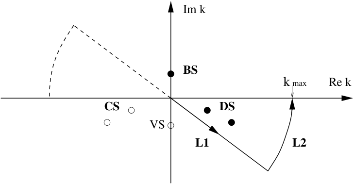
Figure 1: Contour $C_{1}^{+}=L_{1}+L_{2}$ is given by the solid line, while the contour $C_{1}^{-}$ is given by the dashed line. The contour $C_{1}=C_{1}^{+}+C_{1}^{-}$ is clearly inversion symmetric. The two body spectrum which is exposed by this contour is marked by filled circles $\bullet$ and the excluded spectrum by open circles $\circ$. The full spectrum includes bound states (BS), virtual (VS), decay (DS) and capture (CS) resonant states.

For a potential which is analytic in the region above the contour $C_{1}^{+}$ and below the real $k$-axis, we can then derive the transformed Eq. (1) on contour $C_{1}^{+}$

$$\left(\exp{(-2i\theta)}{k^{2}\over 2\mu}-E_{nl}\right)\psi_{nl}(z)+$$

$$\exp{(-3i\theta)}{2\over\pi}\int_{0}^{\infty}dqq^{2}V_{l}(z,z^{\prime})\psi_{nl}(z^{\prime})=0,$$ (6)

where $z=k\exp{(-i\theta)}$ and $z^{\prime}=q\exp{(-i\theta)}$. Eq. (6) is the momentum space version of the complex scaled Schrödinger equation in coordinate space, discussed in e.g., Ref. afnan1 . A rotation in momentum space, $k\exp{(-i\theta)}$, is equivalent to the complex scaling $r\exp{(i\theta)}$ in coordinate space. The phase-transformation $k\>\rightarrow\>k\exp{(-i\theta)}$ is formally a similarity transformation, see for example Ref. brown . The restriction on the rotation angle $\theta$ for the phase-transformation $k\>\rightarrow\>k\exp{(-i\theta)}$ is given by the region of analyticity of the potential. It has been shown in Refs. abc ; abc1 that such a transformation does not alter the location of bound states in the system; the bound state spectrum is invariant under such transformations. This is also clear from the discussion above on completeness relations. The continuum is shifted into the lower-half $k$-plane, while resonant states will occur as long as they are located above the integration contour. The transformed Eq. (6) represents a non-hermitian Hamiltonian. The eigenvalues are therefore in general complex, and the corresponding eigenfunctions form a biorthogonal set with the normalization condition given by Eq. (4).

Next we consider the contour obtained by rotation followed by translation in the lower-half complex $k$-plane. The contour $C^{+}_{2}$ consists of three line segments. The line segment $L_{1}$ is given by a rotation $z_{1}=k_{1}\exp{(-i\theta)}$ where $k_{1}\in[0,b]$, $L_{2}$ is given by a translation $z_{2}=k_{2}-ib\sin(\theta)$ where $k_{2}\in[b\cos(\theta),k_{max}]$ and $b$ determines the translation into the lower-half $k$-plane and $L_{3}$ by $z_{3}=k_{max}-ic$ where $c\in[b\sin(\theta),0]$. For $k_{max}\>\rightarrow\>\infty$ the contribution to the integral in Eq. (1) along the line segment $L_{3}$ will vanish, and the contour $C_{2}^{+}$ reduces to the line segments $L_{1}$ and $L_{2}$. Fig. 2 shows the contour $C_{2}^{+}=L_{1}+L_{2}+L_{3}$ along with the exposed and excluded two-body spectrum which this contour choice implies. The contour $C_{2}^{+}$ is part of the inversion symmetric contour $C_{2}=C_{2}^{+}+C_{2}^{-}$ clearly seen in the figure.

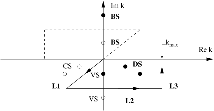
Figure 2: Contour $C_{2}^{+}=L_{1}+L_{2}+L_{3}$ is given by the solid line, while the contour $C_{1}^{-}$ is given by the dashed line. The contour $C_{1}=C_{1}^{+}+C_{1}^{-}$ is clearly inversion symmetric. The two body spectrum which is exposed by this contour is marked by filled circles $\bullet$ and the excluded spectrum by open circles $\circ$. The full spectrum includes bound states (BS), virtual (VS), decay (DS) and capture (CS) resonant states.

We can now transform the momentum space Schrödinger equation (1) onto the distorted contour $C_{2}^{+}$ given by the lines $L_{1}$ and $L_{2}$, i.e., $k,k^{\prime}\>\rightarrow\>z,z^{\prime}$. The integral in Eq. (1) will in this case couple the complex momenta $z_{1}$ and $z_{2}$. The coupled transformed Schrödinger equation then reads

$${1\over 2\mu}\left(\begin{array}[]{cc}z_{1}^{2}&0\\ 0&z_{2}^{2}\end{array}\right)\left(\begin{array}[]{c}\psi_{nl}(z_{1})\\ \psi_{nl}(z_{2})\end{array}\right)+{2\over\pi}\left(\begin{array}[]{cc}\int_{L_{1}}d{z^{\prime}}_{1}\>{z^{\prime}}_{1}^{2}V_{l}(z_{1},{z^{\prime}}_{1})&\int_{L_{2}}d{z^{\prime}}_{2}\>{z^{\prime}}_{2}^{2}V_{l}(z_{1},{z^{\prime}}_{2})\\ \int_{L_{1}}d{z^{\prime}}_{1}\>{z^{\prime}}_{1}^{2}V_{l}(z_{2},{z^{\prime}}_{1})&\int_{L_{2}}d{z^{\prime}}_{2}\>{z^{\prime}}_{2}^{2}V_{l}(z_{2},{z^{\prime}}_{2})\end{array}\right)\left(\begin{array}[]{c}\psi_{nl}({z^{\prime}}_{1})\\ \psi_{nl}({z^{\prime}}_{2})\end{array}\right)=E_{nl}\left(\begin{array}[]{c}\psi_{nl}(z_{1})\\ \psi_{nl}(z_{2})\end{array}\right).$$ (7)

This equation is again a non-hermitian Hamiltonian. The basis of eigenstates forms a biorthogonal set, and the normalization is again given by Eq. (4). The completeness relation given in Eq. (5), will include a discrete sum over bound, virtual and resonant states, and the integration along $L=L_{1}+L_{2}$ is over the complex non-resonant energy continuum.

Fig. 3 shows a plot of the energy spectra of the phase-transformed Eq. (6) and the rotated + translated Eq. (7) in the complex energy plane, for a two-body potential supporting bound and resonant states.

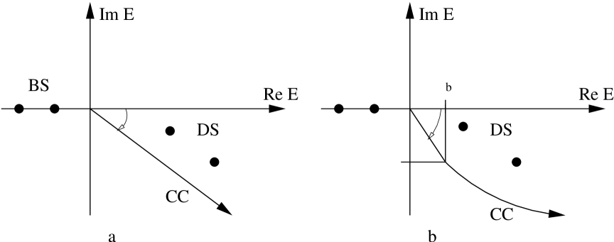
Figure 3: General energy spectra in the complex energy plane for the complex transformed Schrödinger Eqs. (6) and (7), Fig.a and Fig.b, respectively. bound states are denoted by (BS), decay resonant states by (DS) and the complex continuum by (CC).

Whether one chooses to solve the Schrödinger equation on the contour $C_{1}^{+}$ or on the contour $C_{2}^{+}$ depends on the problem under consideration. For potentials which are analytic in the entire lower-half $k$-plane, solving along contour $C_{1}^{+}$ is numerically the most straightforward method. In most cases the potential has singularities in the lower-half $k$-plane, and solving on the contour $C_{2}^{+}$ enables us to avoid the singularities of the potential, while still being able to study resonant structures in the system. Another advantage is that there is no restriction on the rotation angle $\theta$ as long as the contour is chosen so that the poles of the potential are located outside the contour. If a potential is of such an analytic structure that we are allowed to rotate into the third quadrant of the complex $k$-plane (see Fig. 4), virtual states will appear in the calculated spectra, as long as the potential supports virtual states. By solving the Schrödinger equation on the distorted contour $C_{2}^{+}$ rotated into the third quadrant of the complex $k$-plane, we expose a part of the negative imaginary $k$-axis where virtual states may be located, while at the same time excluding a part of the positive imaginary $k$-axis where bound states may be located. This reminds us that the contour should be chosen relative to the partial wave component under study. This means that a separate analysis has to be made for each partial wave.

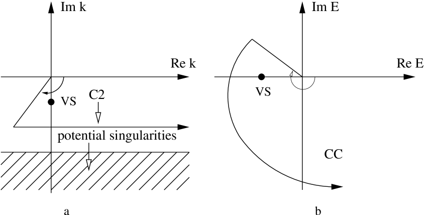
Figure 4: Plot of integration contour $C_{2}^{+}$ where the potential singularities are located in the marked area in Fig. a. The rotation angle $\theta$ is greater than $\pi/2$ and the integration contour encloses a virtual state (A) in the $k$-plane. The corresponding energy spectrum in the complex energy plane in Fig. b illustrates how the virtual state (VS) is exposed in the spectrum and the complex non-resonant continuum (CC).

III Two-body $t$-matrix

In this section we will discuss different procedures for solving the full off-shell $t$-matrix, and hence the full two-body scattering problem. We will consider the general mathematical case where the incoming energy is allowed to take non-physical values, i.e., the input energy is complex. This has relevance for nuclear medium studies where the input energy is in general complex. Two methods for solving the full off-shell $t$-matrix for arbitrary complex energy $\omega$ are outlined.

The $t$-matrix is defined in operator form by

$$t(\omega)=V+VG(\omega)V,$$ (8)

or

$$t(\omega)=V+VG_{0}(\omega)t(\omega).$$ (9)

Here $\omega$ is the incoming energy, $G(\omega)$ is the resolvent, commonly known as the Green’s operator, and $G_{0}(\omega)$ the corresponding free Green’s operator. In operator form they are defined by

$$G_{0}(\omega) = {1\over\omega-H_{0}},$$ (10)

$$G(\omega) = {1\over\omega-H}.$$ (11)

The term $H_{0}$ is the kinetic energy operator and $H$ the full two-body Hamiltonian. By expanding the unit operator on a complete set of physical eigenstates of $H$ given in Eq. (3), we can write the Green’s operator as

$$G(\omega)=\sum_{b}{|\psi_{b}\rangle\langle\psi_{b}|\over\omega-E_{b}}+\int_{0}^{\infty}dE_{c}{|\psi_{c}\rangle\langle\psi_{c}|\over\omega-E_{c}}.$$ (12)

This is the spectral decomposition of the Greens’s function. Here $b$ denotes the discrete bound state spectrum and $c$ the positive energy continuum. By projecting $t(\omega)$ on momentum states, and decomposing into partial waves, the $t$-matrix elements $t_{l}(k,k^{\prime};\omega)$ can be expressed as 1-dimensional integral equations. Depending on whether we start from (8) or (9) we get the spectral or the Fredholm representation of the $t$-matrix. The contour deformation method will be applied to the spectral representation of the $t$-matrix while the solution of the Fredholm representation of the $t$-matrix will be based on the standard principal value prescription.

By using Eq. (8) and Eq. (12) we get the spectral representation of the $t$-matrix by inserting the expansion of the Green’s function on a complete set of states (12), giving

$$t_{l}(k,k^{\prime};\omega)=V_{l}(k,k^{\prime})+{4\over\pi^{2}}\sum_{\alpha}\int_{0}^{\infty}dq\>\int_{0}^{\infty}dq^{\prime}\>q^{2}{q^{\prime}}^{2}V_{l}(k,q){\psi_{\alpha}(q)\psi_{\alpha}^{*}(q^{\prime})\over\omega-E_{\alpha}}V_{l}(q^{\prime},k^{\prime}).$$

The sum over $\alpha$ implies a discrete sum over bound states and an integration over the positive energy continuum. Eq. (III) is analytic along the real energy axis, except for poles located at bound state energies and a branch cut along the positive energy axis. In physical two-body scattering the incoming energy is defined on the positive real energy axis. In this case the integrand in Eq. (III) is singular, and a numerical solution of Eq. (III) is highly non-trivial. However, for negative real input energies it can be solved by standard numerical procedures.

We are however interested in the $t$-matrix for arbitrary complex energies, since an obvious extension of this work is to consider in-medium scattering of two nucleons or to study the resummation of large classes of many-body diagrams. In a nuclear medium calculation the self-consistently determined quasiparticle energies are in general complex.

We can achieve this by an analytic continuation of the contour integrals into the complex $k$-plane. This represents a deformation of the integration contour in the complex $k$-plane. See Refs. kukulin ; nuttal1 for validity and mathematical proofs concerning analytic continuation of integral equations.

We will consider the solution of Eq. (III) by integrating over the two contours, $C_{1}^{+}$ or $C_{2}^{+}$, discussed in Sec. II, resulting in the following expression for $t_{l}(k,k^{\prime};\omega)$

$$t_{l}(k,k^{\prime},\omega)=V_{l}(k,k^{\prime})+{4\over\pi^{2}}\sum_{\alpha}\int_{C}\int_{C^{\prime}}dz\>d{z^{\prime}}\>z^{2}{z^{\prime}}^{2}V_{l}(k,z){\psi_{\alpha}(z)\psi_{\alpha}(z^{\prime})\over\omega-E_{\alpha}}V_{l}(z^{\prime},k^{\prime}),$$

Here $C$ is either $C_{1}^{+}$ or $C_{2}^{+}$. This applies to $C^{\prime}$ as well. We have expanded the Green’s operator (11) on the basis given in Eq. (5), this implies that $\alpha$ represents discrete bound, virtual and resonant states and a non-resonant complex energy continuum. From the mathematical structure of Eq. (III) it is easily seen that the $t$-matrix is analytic in $\omega$ in the entire complex energy-plane except for poles located at bound, virtual and resonant state energies. In addition there could also be singularities in the potential itself. The numerical method for solving Eq. (III) is based on matrix diagonalization. We first have to diagonalize the corresponding Schrödinger equation, and then expand the Green’s function on the discretized basis obtained.

Applying this method enables us to obtain $t_{l}(k,k^{\prime};\omega)$ for both real and complex energies $\omega$. The integral becomes non-singular on the deformed contour for real and positive input energies $\omega$, resulting in numerically stable solutions for physical two-body scattering. Eq. (III) can also be considered as an analytic continuation of Eq. (III) for complex input energies $\omega$, and stable numerical solution can be obtained for complex energies above the distorted contour. The limitation of this method is due to that most potentials in momentum space have singularities in the complex plane when one argument is real and the other is complex. By applying contour $C_{1}^{+}$, which is based on rotation into the complex plane, in most cases there will be restrictions on both rotation angle ($\theta$) and maximum incoming and outgoing momentum ($k,k^{\prime}$), see for example Ref. nuttal .

Using contour $C_{2}^{+}$ we can avoid these limitations by choosing the integration contour in such a way that the potential singularities always will lie outside the integration contour, and therefore do not give any restriction on rotation angle and maximum incoming and outgoing momentum.

The partial wave decomposition of Eq. (9) gives the Fredholm representation, commonly known as the Lippmann-Schwinger equation

$$t_{l}(k,k^{\prime};\omega)=V_{l}(k,k^{\prime})+{2\over\pi}\int_{0}^{\infty}{dqq^{2}V_{l}(k,q)t_{l}(q,k^{\prime})\over\omega-E(q)}.$$ (13)

In physical two-body scattering the input energy is real and positive. In this case the Fredholm integral Eq. (13) has a singular kernel of Cauchy type. Solving singular integrals can be done by Cauchy’s Residue theorem, where we integrate over a closed contour enclosing the poles. There are two ways of doing this, either by letting $z$ lie an infinitesimal distance above the real axis, i.e., $\omega\rightarrow z+i\epsilon$, or by letting $\omega$ lie on the real axis. In both cases we must choose a suitable contour enclosing the singularity. If we choose the latter position of the singularity, we get a Cauchy principal-value integral where we integrate up to - but not through - the singularity, and a second contour integral, where the contour can be chosen as a semicircle around the singularity. Eq. (13) can thus be given in terms of a principal value part and a second term coming from integration over the semicircle around the pole. The result is

$$t_{l}(k,k^{\prime};\omega)=V_{l}(k,k^{\prime})+{2\over\pi}\mathcal{P}\int_{0}^{\infty}{dqq^{2}V_{l}(k,q)t_{l}(q,k^{\prime})\over\omega-E(q)}\>-\>2i\mu k_{0}V_{l}(k,k_{0})t_{l}(k_{0},k^{\prime};\omega).$$ (14)

By rewriting the principal value integral using the relation

$$\mathcal{P}\int_{0}^{\infty}dk\>{f(k)\over k_{0}^{2}-k^{2}}=\int_{0}^{\infty}dk\>{[f(k)-f(k_{0})]\over k_{0}^{2}-k^{2}},$$ (15)

we obtain an equation suitable for numerical evaluation. Eq. (14) can be converted into a set of linear equations by approximating the integral by a sum over $N$ Gaussian quadrature points $(k_{j};j=1,...N)$, each weighted by $w_{j}$ The full off-shell $t$-matrix is then obtained by matrix inversion. This method for solving integral equations is known as the Nystrom method. It is numerically effective and stable, except for the rare case when the incoming energy $\omega$ coincides with or is very close to one of the integration points.

So far we have only considered physical input energies in Eq. (13), but it has been shown in Ref. kukulin that the analytically continued Lippmann-Schwinger equation to complex energies takes the same form as Eq. (14). By solving the full off-shell $t$-matrix for arbitrary complex input energy, we do not have to alter the set of linear equations obtained for physical energy, the only modification is that the energy is complex. It should be noted that the Lippmann-Schwinger equation (III) can be solved by the contour deformation method as well, giving a compact integral kernel for positive incoming energies. By contour distortion the principal value prescription is avoided, and a numerical solution of Eq. (III) is stable even for incoming energies coinciding with the integration points.

IV An analytically solvable two-body potential

We now consider a separable potential given by Yamaguchi yamaguchi . It models $s$- and $p$-waves. A separable interaction in momentum space is analytically solvable, see for example Ref. newton for a demonstration. The Yamaguchi interaction therefore admits analytical solution of the full off-shell $t$-matrix and the $t$-matrix poles, corresponding to the energy spectrum. The Yamaguchi $s$-wave potential supports bound and virtual states, while the Yamaguchi $p$-wave potential supports bound, virtual and resonant states. The Yamaguchi potential is therefore very useful in modelling loosely bound two-body systems which may have a rich resonant state structure, and for checking the numerics in our calculations of the $t$-matrix and the energy spectrum.

The $s$-wave Yamaguchi potential has the form

$$V_{0}(k,q)=-\lambda g_{0}(k)g_{0}(q),$$ (16)

where

$$g_{0}(k)={1\over k^{2}+\beta^{2}}.$$ (17)

In natural units and mass $2\mu=1$ MeV, the full off-shell $t$-matrix for the $s$-wave potential reads newton

$$t_{0}(k,q;z)=-\lambda{g_{0}(k)g_{0}(q)\over 1-\lambda{2\over\pi}\int_{0}^{\infty}dk\>{k^{2}\over k^{2}-E}{1\over(k^{2}+\beta^{2})}}.$$ (18)

The integral in the denominator can be evaluated, giving

$$\lambda{2\over\pi}\int_{0}^{\infty}dk\>{k^{2}\over k^{2}-E}{1\over(k^{2}+\beta^{2})}={\lambda\over 2}{(\beta+i\sqrt{E})^{2}\over\beta(\beta^{2}+E)^{2}}.$$ (19)

The $s$-wave $t$-matrix in closed form reads

$$t_{0}(k,q;E)=-\lambda{g_{0}(k)g_{0}(q)\over 1-{\lambda\over 2}{(\beta+i\sqrt{E})^{2}\over\beta(\beta^{2}+E)^{2}}}.$$ (20)

Writing $\kappa=-ik$ where $E=k^{2}$ we can solve for the $t$-matrix poles as zeroes of the denominator

$$1-{\lambda\over 2}{(\beta-\kappa)^{2}\over\beta(\beta^{2}-\kappa^{2})^{2}}=0.$$ (21)

Solving for $\kappa$ gives

$$\kappa=-\beta\pm\sqrt{{\lambda\over 2\beta}},$$ (22)

and we see that the poles are located along the imaginary $k$-axis. Poles of the $t$-matrix located on the positive imaginary $k$-axis represents bound states, while poles located on the negative imaginary $k$-axis represents virtual states, giving a bound $(\kappa>0)$ and a virtual state $(\kappa\leq 0)$ for $\lambda>2\beta^{3}$ and for $\lambda\leq 2\beta^{3}$ two virtual states.

The separable $p$-wave interaction is given by

$$V_{1}(k,q)=-\lambda g_{1}(k)g_{1}(q),$$ (23)

where

$$g_{1}(k)={k\over k^{2}+\beta^{2}},$$ (24)

and the $t$-matrix now becomes newton

$$t_{1}(k,q;E)=-\lambda{g_{1}(k)g_{1}(q)\over 1-\lambda{2\over\pi}\int_{0}^{\infty}dk\>{k^{2}\over k^{2}-E}{k^{2}\over(k^{2}+\beta^{2})^{2}}}.$$ (25)

Solving again the integral in the denominator gives the $t$-matrix in closed form

$$t_{1}(k,q;E)=-\lambda{g_{1}(k)g_{1}(q)\over 1-{\lambda\over 2}{\beta^{3}+E(3\beta+2i\sqrt{E})\over(\beta^{2}+E)^{2}}},$$ (26)

and solving for the poles gives in terms of $\kappa=-ik$

$$\kappa={\lambda\over 2}-\beta\pm{1\over 4}\sqrt{4\lambda^{2}-8\lambda\beta}.$$ (27)

We see that for $p$-waves the interaction supports bound, virtual and resonant states. The bound state condition is

$$\lambda>{2\beta}.$$ (28)

giving in addition a virtual state. The interaction has a branchpoint at $k=0$ where the bound and virtual state meet and move symmetrically from the imaginary axis into the lower-half $k$-plane giving capture and decay resonant states. Fig. 5 shows the pole trajectory for the Yamaguchi $p$-wave interaction.

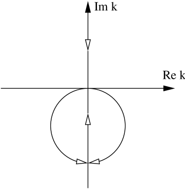
Figure 5: Pole trajectory for the $p$-wave Yamaguchi interaction in the complex $k$-plane.

V Numerical results

Below we present numerical calculations for the complete energy spectrum of the separable Yamaguchi potential yamaguchi , for the Malfliet-Tjon malfliet and the realistic charge dependent Bonn (CD-Bonn) machleidt nucleon-nucleon interactions. We also present calculations of the $t$-matrix for the given interactions within the formalism outlined above. The analytic structure of the various interactions is of importance for the choice of the integration contour in the complex plane, as will be discussed.

V.1 Results for the Yamaguchi potential

The Yamaguchi potential is analytic in the entire complex $k$-plane except for singularities located at $k,k^{\prime}=\pm i\beta$, arising from the separable part of the potential $1/(k^{2}+\beta^{2})$. This singularity gives a restriction on the integration contour; if we consider the rotated contour $C_{1}^{+}$, the rotation angle $\theta$ has to be less than $\pi/2$, i.e., $\theta<\pi/2$, in the complex $k$-plane. This contour choice will not be able to give the virtual states in the calculated energy spectrum. The contour $C_{2}^{+}$ could on the other hand be chosen to lie above the singularity, i.e., $b\sin(\theta)<\beta$. By this choice there is no restriction on the rotation angle $\theta$ and we can rotate into the third quadrant of the complex $k$-plane. By this procedure virtual states can be included in the calculated energy spectrum.

In Table 1 we present numerical versus exact values for the $s$-wave virtual states in the Yamaguchi potential, using contour $C_{2}^{+}$. The contour $C_{2}^{+}$ was rotated $\theta=2\pi/3$ into the third quadrant and translated $c=5\sin(2\pi/3)\approx 4.3301$ MeV in the lower-half complex $k$-plane. Fig. 6 shows the contour along with the excluded spectrum and the singularities of the $s$-wave Yamaguchi potential giving restrictions on the contour choice. The parameter $\beta$ was held fixed, and equal to $\beta=6$ MeV. The potential depth $\lambda$ was chosen to give only virtual states. The contour choice exposes one virtual state while one virtual state will be excluded from the calculated spectrum. The calculations used $N1=50$ integration points along line $L_{1}$ and $N2=50$ integration points along $L_{2}$

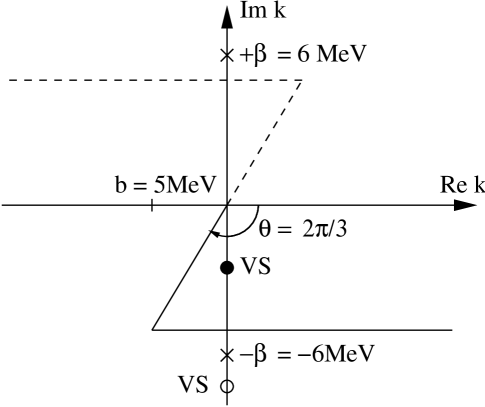
Figure 6: Excluded ($\circ$) and included ($\bullet$) spectrum for the $s$-wave Yamaguchi potential, with $\beta=6$ MeV and $\lambda$ chosen to give only virtual states (VS) in the full spectrum. The calculation of the spectrum for this contour choice is given in Table 1. Potential singularites are given by ($\times$) in the figure.

In Table  2 and Table 3 we present numerical versus exact values of the $p$-wave energy spectra, calculated using contour $C_{2}^{+}$ and $C_{1}^{+}$. The calculations used $N1=50$ integration points along line $L_{1}$ and $N2=50$ integration points along $L_{2}$ for contour $C_{2}^{+}$. For the contour $C_{1}^{+}$ a number of $N=100$ integration points was used. The rotation angle is the same for both contours and equal to $\theta=\pi/6$. The parameter $\beta$ in the potential was held fixed, and equal to $\beta=6$ MeV. The translation parameter of contour $C_{2}^{+}$ is given by $b=3.5$ MeV. Fig. 7 shows the contour along with the excluded and included spectrum for the contour $C_{1}^{+}$ and the contour $C_{2}^{+}$, along with the singularities of the $p$-wave Yamaguchi potential giving restrictions on the contour choice.

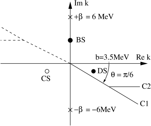
Figure 7: Excluded ($\circ$) and included ($\bullet$) spectrum for the $p$-wave Yamaguchi potential, with $\beta=6$MeV and $\lambda$ chosen to give bound (BS), virtual (VS), capture (CS) and decay (DS) states in the full spectrum. The calculations of the spectrum for contour $C_{1}^{+}$ ($C1$) and contour $C_{2}^{+}$ ($C2$) are given in Tables 2 and 3, respectively. Potential singularites are given by ($\times$) in the figure.

	Exact	Contour    $C_{2}^{+}$
$\lambda$	Real	Real
200	-3.67687178	-3.67687178
250	-2.06107759	-2.06107759
300	-1.00000000	-1.00000000
350	-0.35925969	-0.35925969
390	-0.08947449	-0.08947449

Table 1: Numerical calculations for the Yamaguchi $s$-wave virtual states versus exact values. Energies are given in units of MeV. The numerical calculations were obtained using the contour deformation method (CDM) along contour $C_{2}^{+}$.

	Exact		Contour $C_{2}^{+}$
$\lambda$	Real	Imag.	Real	Imag.
13	-5.30277586	0	-5.30277586	0.
12.6	-2.80486369	0	-2.80486369	0.
12.2	-0.77620500	0	-0.77620500	0.
11.8	0.57999998	-0.15362291	0.57999998	-0.15362291
11.7	0.85500001	-0.28102490	0.85500001	-0.28102490
11.5	1.37500000	-0.59947896	1.37500000	-0.59947896
11.0	2.50000000	-1.65831244	2.50000000	-1.65831244

Table 2: Numerical calculations for the Yamaguchi $p$-wave bound and resonant energy spectra versus exact values. Energies are given in units of MeV. The numerical calculations were obtained using the contour deformation method (CDM) along contour $C_{2}^{+}$.

	Exact		Contour $C_{1}^{+}$
$\lambda$	Real	Imag.	Real	Imag.
13	-5.30277586	0	-5.30277563	0.
12.6	-2.80486369	0	-2.80486362	0.
12.2	-0.77620500	0	-0.77620499	0.
11.8	0.57999998	-0.15362291	0.57999998	-0.15362291
11.7	0.85500001	-0.28102490	0.85500001	-0.28102490
11.5	1.37500000	-0.59947896	1.37500000	-0.59947896
11.0	2.50000000	-1.65831244	2.50000000	-1.65831244

Table 3: Numerical calculations for the Yamaguchi $p$-wave bound and resonant state energy spectra versus exact values. Energies are given in units of MeV. The numerical calculations were obtained using the contour deformation method (CDM) along contour $C_{1}^{+}$.

The results for the virtual states for the $p$-wave Yamaguchi potential using contour $C_{2}^{+}$, are given in Table 4.

	Exact	Contour    $C_{2}^{+}$
$\lambda$	Real	Real
13	-1.69722438	-1.69722438
12.6	-1.15513635	-1.15513635
12.2	-0.46379500	-0.46379500
12.1	-0.25000000	-0.25000000

Table 4: Numerical calculations for the Yamaguchi $p$-wave virtual state energy spectra versus exact values. Energies are given in units of MeV. The numerical calculations were obtained using the contour deformation method (CDM) along contour $C_{1}^{+}$ with $\theta>\pi/2$. See Fig. 6 for a plot of the contour $C_{2}^{+}$.

We conclude that there is no difference between the numerically calculated and the exact bound, virtual and resonant energy spectra. To see a difference for the number of integration points used in the calculations we have to include up two 12 significant digits. Using double precision we get for the $p$-wave ($\lambda=13$) virtual state the exact value $E=-1.697224362268005$ MeV while the numerical result in double precision is $E=-1.697224362276472$ MeV. The calculated results for resonant states with large widths, i.e., far from the real energy axis agree perfectly with exact values. This illustrates the advantage of the contour deformation method in momentum space as opposed to the complex scaling analog in coordinate space, where convergence of these states will expectedly be slower due to the slowly decreasing oscillating wavefunctions. Fig. 8 gives a plot of the calculated energy spectrum for the $p$-wave Yamaguchi potential, using contours $C_{1}^{+}$ and $C_{2}^{+}$. Contour $C_{1}^{+}$ is rotated by $\theta=2\pi/5$ in the energy plane while contour $C_{2}^{+}$ is rotated into the third quadrant of the complex $k$-plane by $\theta=3\pi/5$ giving a rotation of $\theta=6\pi/5$ in the energy plane. The resonant state appears at the same location for both contours.

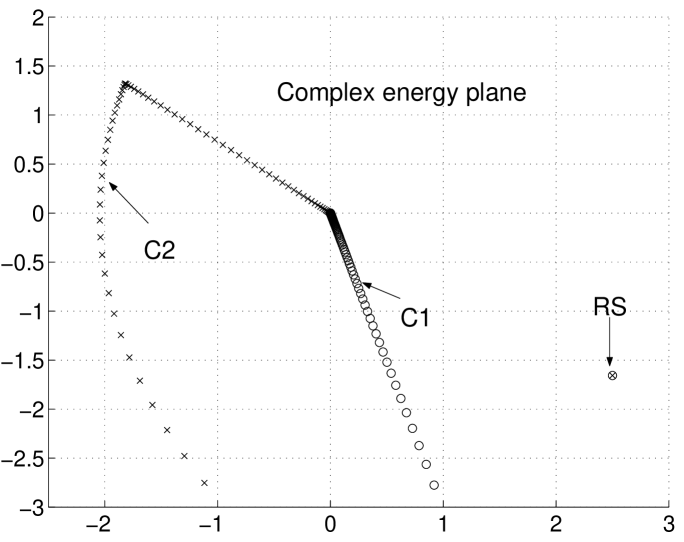
Figure 8: Calculated energy spectra for the $p$-wave Yamaguchi potential with parameters $\lambda=11$, $\beta=6$ using the contours $C_{1}^{+}\>(C1),C_{2}^{+}\>(C2)$. The discretized non-resonant continuum lies along the contours, and a resonant state (RS) appears in the energy spectra.

Next we present a calculation of the $t$-matrix elements $t_{l}(k,k;E)$ for both real and complex input energy (see Table  5 and Table 6 ) for the $p$-wave Yamaguchi potential. The $t$-matrix is calculated by applying the spectral representation on the deformed contour $C_{2}^{+}$. The contour is rotated into the third quadrant of the complex $k$-plane and the difference between numerical calculations and exact values is of the same order as for the calculations of the energy spectrum. The rotation, translation and number of integration points were the same as above.

	Exact		Contour $C_{2}^{+}$
$k$	Real	Imag.	Real	Imag.
1.5	0.102303714	-0.061759732	0.102303714	-0.061759732
3	0.295657724	-0.178485632	0.295657724	-0.178485632
4	0.425747126	-0.257019311	0.425747126	-0.257019311
6	0.461965203	-0.278883785	0.461965203	-0.278883785
7.5	0.439705133	-0.265445620	0.439705133	-0.265445620
9	0.393627137	-0.237628803	0.393627137	-0.237628803
10	0.342892975	-0.207001090	0.342892975	-0.207001090

Table 5: Calculation of the $p$-wave ($l=1$) $t_{l}(k,k,E)$ for real momenta $k$ and input energy $E=5$ MeV. $t_{l}(k,k,E)$ is given in units of MeV^-2. The interaction parameters are $\lambda=12.5$, $\beta=6$ MeV, the rotation angle is $\theta=2\pi/3$ while the translation is given by $b=3.5$ MeV. The number of integration points was $N1=N2=50$

	Exact		Contour $C_{2}^{+}$
$k$	Real	Imag.	Real	Imag.
1.5	0.094043918	-0.030566057	0.094043918	-0.030566057
3	0.271786928	-0.088335901	0.271786928	-0.088335901
4.5	0.391373158	-0.127203703	0.391373158	-0.127203703
6	0.424667060	-0.138024852	0.424667060	-0.138024852
7.5	0.404204220	-0.131374046	0.404204220	-0.131374046
9	0.361846477	-0.117606975	0.361846477	-0.117606975
10.5	0.315208495	-0.102448739	0.315208495	-0.102448739

Table 6: Calculation of the $p$-wave $t_{l}(k,k,E)$ for real momenta $k$ and complex input energy $E=5-2i$ MeV. $t_{l}(k,k,E)$ is given in units of MeV^-2. Interaction parameters are $\lambda=12.5$, $\beta=6$ MeV , the rotation angle is $\theta=2\pi/3$ while the translation is given by $b=3.5$ MeV. The number of integration points was $N1=N2=50$.

V.2 Results for the Malfliet-Tjon interaction

The Malfliet-Tjon interaction malfliet is a superposition of Yukawa terms. This interaction resembles the form of a realistic nucleon-nucleon interaction with attractive and repulsive parts in the ${}^{1}S_{0}$ channel. It can be fitted to reproduce the ${}^{1}S_{0}$ phase shift in nucleon- nucleon scattering rather well. The interaction in coordinate representation is given by

$$V(r)=V_{A}{\exp{(-\mu_{A}r)}\over r}+V_{B}{\exp{(-\mu_{B}r})\over r}.$$ (29)

This interaction will support bound and virtual states for $s$-waves, while for higher angular momentum resonances will appear. It is known that the ${}^{1}S_{0}$ channel in the nucleon-nucleon interaction supports a virtual state near the scattering threshold.

We will only consider $s$-waves and calculate the energy spectrum using contour $C_{2}^{+}$ rotated into the third quadrant of the complex $k$-plane. First we consider the analytic structure of the Malfliet-Tjon interaction in momentum space. The Fourier-Bessel transform of (29), for the $s$-wave, is

$$V_{0}(k,k^{\prime}) = V_{A}{1\over 4kk^{\prime}}\ln\left({(k+k^{\prime})^{2}+\mu_{A}^{2}\over(k-k^{\prime})^{2}+\mu_{A}^{2}}\right)$$ (30)

$$+ V_{B}{1\over 4kk^{\prime}}\ln\left({(k+k^{\prime})^{2}+\mu_{B}^{2}\over(k-k^{\prime})^{2}+\mu_{B}^{2}}\right).$$

By analytic continuation of the interaction (30) to the complex $k$-plane, there will be singularities in the interaction for

$$(z-z^{\prime})^{2}+\mu_{A,B}^{2}=0,$$ (31)

and

$$(z+z^{\prime})^{2}+\mu_{A,B}^{2}=0.$$ (32)

Eq. (31) is only satisfied if one of the arguments is real and the other complex. For $z^{\prime}=k^{\prime}$ real, we have singularities for $\Re[z]=\mp k^{\prime}\>\wedge\>\Im[z]=\pm\mu$. Eq. (32) is satisfied for $(z+z^{\prime})=\pm i\mu_{A,B}$, which gives $\Re[z]=\Re[z^{\prime}]\>\wedge\>\Im[z]=\pm\mu_{A,B}-\Im[z^{\prime}]$. Solving the eigenvalue problem by the contour deformation method on the purely rotated contour $C_{1}^{+}$, singularities appear along the imaginary axis given by $\Im[z]=\pm\mu_{A,B}-\Im[z^{\prime}]$. This gives a restriction on rotation angle, $\theta<\pi/2$. This does not allow a rotation into the third quadrant of the complex $k$-plane, and calculation of virtual states is not possible by this contour choice. This problem is resolved by solving the eigenvalue problem on the rotated + translated contour $C_{2}^{+}$. For a rotation angle $\theta\geq\pi/2$ singularities appear on the contour $C_{2}^{+}$ for $\Re[z]=\Re[z^{\prime}]\>\wedge\>\Im[z]+\Im[z^{\prime}]=\pm\mu_{A,B}$. By imposing a lower bound on the translated line segment $L_{2}$, given by $c<\mu_{A,B}/2$, we avoid all singularities. By this choice, rotation into the third quadrant of the complex $k$-plane is allowed, and an exploration of virtual states is possible.

If we want to extract the $t$-matrix along the real $k$-axis by the contour deformation method, see Sec. III, singularities appear when Eq. (31) is satisfied. If we integrate along contour $C_{1}^{+}$ there will always be a singularity on the contour given by

$$z=k_{max}-i\mu,$$ (33)

where

$$k_{max}=\mu/\tan(\theta),$$ (34)

and $\mu=min[\mu_{A},\mu_{B}]$. For $k,k^{\prime}>k_{max}$ the contour $C_{1}^{+}$ will pass through the singularity of the interaction and Cauchy’s integral theorem cannot be applied. However, if the interaction, $V_{l}(k,k^{\prime})$, is approximately zero for $k,k^{\prime}>k_{max}$ integrating along contour $C_{1}^{+}$ can be done as long as

$$\theta<\arctan\left(\mu/k_{max}\right).$$ (35)

In this sense we may call $k_{max}$ the cutoff momentum. This choice may cause numerical unstable solutions for small values of momenta, since the rotated contour may lie very close to the real $k$-axis where the integral kernel is singular. The same conclusion has already been pointed out in Ref. nuttal .

Here we see the advantage of integrating along contour $C_{2}^{+}$; Not only will it be able to reproduce virtual states in the spectra, but it will also give accurate calculations of the $t$-matrix for real incoming and outgoing momentum. It will always be possible to choose a contour $C_{2}^{+}$ lying above the nearest singularity $z=\Re[k]-i\mu$, implying no restriction on rotation angle $\theta$ irrespective of cutoff momentum $k_{max}$. Fig. 9 gives an illustration.

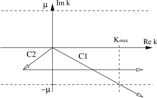
Figure 9: Illustration of potential singularities for the Malfliet-Tjon interaction $V_{l}(k,z^{\prime})$, where $k$ is real and $z^{\prime}$ complex. Restriction on the integration contours $C_{1}^{+}\>(C1)$ and $C_{2}^{+}\>(C2)$ is clearly seen for given cutoff momentum $k_{max}$ ($V_{l}(k,k^{\prime})\approx 0$ for $k,k^{\prime}>k_{max}$).

A calculation of resonant and virtual states in the Malfliet-Tjon interaction is given in Ref. elster . The $t$-matrix poles were calculated by analytic continuation of the $t$-matrix to the second energy sheet, and thereby searching for poles. In Table 7 a calculation of the virtual neutron-proton $s$-wave states with reduced mass $M_{np}=938.926$ MeV and $\hbar=c=1$ for interaction parameters $V_{A}=7.291$ MeV, $\mu_{A}=613.69$ MeV, $\mu_{B}=305.86$ MeV held fixed while $V_{B}$ was varied as given in Table 7. The rotation is $\theta=2\pi/3$ and the translation $c=100\sin(2\pi/3)$ MeV. The convergence is illustrated by increasing the number of integration points.

	CDM			Ref.elster
	A	B	C	D
$V_{B}$	Energy	Energy	Energy	Energy
-2.6047	-0.066674	-0.066653	-0.066653	-0.06663
-2.5	-0.310114	-0.310115	-0.310115	-0.31004
-2.3	-1.229845	-1.229845	-1.229845	-1.22970
-2.1	-2.679069	-2.678979	-2.678979	-2.67878

Table 7: Calculation of the neutron-proton virtual state as function of interaction parameter $\lambda$ for the $s$-wave Malfliet-Tjon interaction using the deformed integration contour $C_{2}^{+}$. The convergence is illustrated by increasing the number of integration points. Column A used N1 = 30, N2 = 50 integration points, column B used N1 = 100, N2 = 100 integration points and column C used N1 = 150, N2 = 250 integration points. Comparison is made with the calculations of Ref. elster , given in column D.

We see a small difference in the calculated values for the virtual state in the Malfliet-Tjon interaction. As we obtained convergence of the virtual state energies by increasing the number of integration points, this suggests that our results are stable. Fig. 10 shows a plot of the calculated $t$-matrix elements $t_{l}(k,k;E)$ for incoming energy $E=100$ MeV for the $s$ -wave Malfliet-Tjon interaction, using the contours $C_{1}^{+}$ and $C_{2}^{+}$. In this case we used a rotation angle $\theta=\pi/6$ for both contours, and a translation $b=300$ MeV for contour $C_{2}^{+}$. The Malfliet-Tjon interaction has a singularity along contour $C_{1}^{+}$, given by $k_{max}=\mu/\tan(\theta)=529.77$ MeV. In this case the interaction is not sufficiently neglible for $k,k^{\prime}>k_{max}$, and using contour $C_{1}^{+}$ will not give accurate calculation of the $t$-matrix, this is clearly seen in the plot of the calculated results.

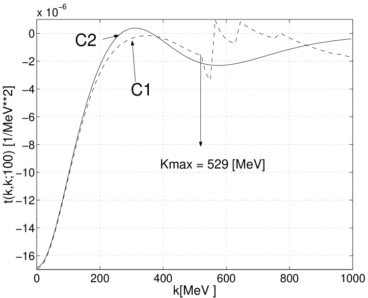
Figure 10: Plot of $t$-matrix elements for the $s$-wave Malfliet-Tjon interaction using the contour $C_{1}^{+}$ (dashed line) and the contour $C_{2}^{+}$ (solid line). The potential singularity along contour $C_{1}^{+}$ is clearly displayed, and located at $k_{max}=529.77$ MeV.

This illustrates clearly the advantage of integrating along the contour $C_{2}^{+}$ instead of $C_{1}^{+}$.

A useful check of the numerics is the on-shell unitarity for the $S$-matrix. Table  8 reports calculations done by the principal-value prescription and the contour deformation method $C_{2}^{+}$. We used $N=50$ integration points for the principal value integration, for the contour deformation method we used $N1=30$ and $N2=100,200$. We observe that we need a higher number of integration points along line $L_{2}$ for obtaining convergence.

	PV	CDM
$k$[MeV]	$N=50$	$N2=100$	$N2=200$
10.	1.00000000	1.00000811	1.00000811
110.	1.00000000	0.999999940	1.00000000
210.	1.00000000	0.999999940	1.00000000
310.	1.00000000	0.999999881	1.00000000
410.	1.00000000	0.999999881	1.00000000
510.	1.00000000	0.999999881	1.00000000
610.	1.00000000	0.999999881	1.00000000
710.	1.00000000	0.999999821	1.00000000
810.	1.00000000	0.999999821	1.00000000
910.	1.00000000	0.999999821	1.00000000
1010.	1.00000000	0.999999762	1.00000000
1110.	1.00000000	0.999999702	1.00000000
1210.	1.00000000	0.999999702	1.00000000
1310.	1.00000000	0.999999642	1.00000000
1410.	1.00000000	0.999999523	1.00000000
1510.	1.00000000	0.999999642	1.00000000

Table 8: Calculations of $S$-matrix norm, $|S(k)|$, for the $s$-wave Malfliet-Tjon potential with parameters $V_{A}=7.291$ MeV, $\mu_{A}=613.69$ MeV, $V_{B}=-5$ MeV and $\mu_{B}=305.86$ MeV. Column 2 gives results for the principal value prescription (PV), while columns 3,4 give results for the contour deformation method (CDM).

V.3 Results for the CD-Bonn nucleon-nucleon interaction

Finally, we present a calculation of the energy spectrum of the charge-dependent Bonn interaction (CD-Bonn) and phase shifts for a set of selected partial waves. The CD-Bonn interaction is given in Ref. machleidt . We illustrate the power of the contour deformation method by reproducing the deuteron bound state and the virtual states in the ${}^{1}S_{0}$ isospin triplet channel. In addition, phase shifts are calculated within the same method, and the results agree perfectly with other theoretical predictions.

The tensor component of the CD-Bonn interaction couples angular momentum, $l=j-1,l=j+1$, in the spin triplet channel. It is straightforward to include this coupling in the formalism outlined in the previous sections. Instead of $N$x$N$ matrices we get $2N$x$2N$ matrices in the coupled case, for the uncoupled channels we still have $N$x$N$ matrices. We should of course label the equations with quantum numbers $L,S,J,T$.

The realistic nucleon-nucleon interaction does not have a resonant structure in the low energy region $E<350$ MeV. It does however support virtual states in the ${}^{1}S_{0}$ isospin triplet channel and a bound state in the coupled isospin singlet channel (the deuteron) ${}^{3}S_{1}-{}^{3}D_{1}$. We compare the calculated virtual state locations in the complex $k$-plane with the values obtained by the effective range approximation, see Ref. newton ; kukulin . In the following we do not include Coulomb effects when considering the isospin $t_{z}=-1$ channel (proton-proton scattering).

The effective range approximation for the $s$-wave poles is given by

$$k=i\left[{1\over r_{NN}}-\sqrt{{2\over r_{NN}|a_{NN}|}+{1\over r_{NN}^{2}}}\right].$$ (36)

The theoretical (see below) and experimental values machleidt for the ${}^{1}S_{0}$ scattering lengths $a_{NN}$ and effective range $r_{NN}$ are given in Table 9

	CD-Bonn	Experiment
$a_{pp}$	$-17.4602$
$r_{pp}$	2.845
$a_{nn}$	-18.9680	-18.9 $\pm$0.4
$r_{nn}$	2.819	2.75 $\pm$0.11
$a_{np}$	-23.7380	-23.740 $\pm$0.020
$r_{np}$	2.671	2.77 $\pm$0.05

Table 9: Scattering lengths (a) and effective ranges (r) for the ${}^{1}S_{0}$ channel, in units of fm. For the proton - proton channel Coulomb effects are not included.

To apply the contour deformation method by integrating along contour $C_{2}^{+}$ we first have to locate possible singularities in the CD-Bonn interaction. The CD-Bonn interaction is given explicitly in momentum space. The derivation of the interaction is based on field theory, starting from Lagrangians describing the coupling of the various mesons of interest to nucleons machleidt . The one-boson-exchange interaction is proportional to

$$V({\bf k,q})\propto\sum_{\alpha=\pi^{0},\pi^{\pm},\rho,\omega,\sigma_{1},\sigma_{2}}\bar{V}_{\alpha}({\bf k,q})F_{\alpha}^{2}({\bf k,q};\Delta_{\alpha}).$$ (37)

Both $\bar{V}_{\alpha}({\bf k,q})$ and $F_{\alpha}^{2}({\bf k,q};\Delta_{\alpha})$ contain terms of the form

$${1\over({\bf k-q})^{2}+m_{\alpha}^{2}},$$ (38)

which are of the Yukawa type. These terms determine the analyticity region of the interaction in the $k$-plane (see discussion of the Malfliet-Tjon interaction above. We see that the poles of the interaction are determined by the various meson masses $m_{\alpha}$ and cut-off masses $\Delta_{\alpha}$. Considering the solution of the eigenvalue problem by the contour deformation method using contour $C_{2}^{+}$, singularities in the interaction appear for $\theta\geq\pi/2$, i.e., a rotation into the third quadrant of the complex $k$-plane. The maximum translation into the complex $k$-plane is then determined by the smallest meson mass entering the potential, which is the $\pi$-meson, $m_{\pi^{0}}=134.9764$ MeV. For a given rotation into the third quadrant, i.e., $\theta\geq\pi/2$, we get a restriction on the translation parameter; $b<134.9764/2\sin(\theta)$. Here $b$ is given in MeV, as we are still using natural units.

Table 10 gives results for the virtual states in the ${}^{1}S_{0}$ channel by the contour deformation method. A comparison with the effective range calculation of the virtual state poles is also shown. The contour was rotated by $\theta=2\pi/3$ into the complex $k$-plane and translated $c=-30\sin(5\pi/7)$ MeV or $c\approx-23.45$ MeV in the lower-half $k$-plane. This is sufficient to reproduce the virtual states in the ${}^{1}S_{0}$ channel, as they are known to lie very close to the scattering threshold, $k\approx-\hbar c0.05i$ MeV. By this contour choice the full energy spectrum is obtainable since it is known a posteriori that the ${}^{1}S_{0}$ channel supports only virtual states near the scattering threshold. The convergence of the numerical calculated values is demonstrated by increasing the number of integration points $N$.

	CDM			EFR
	a	b	c
$T_{z}$	Energy	Energy	Energy	Energy
-1 (pp)	-0.11766	-0.11761	-0.11761	-0.11763
1 (nn)	-0.10070	-0.10069	-0.10069	-0.10070
0 (np)	-0.06632	-0.06632	-0.06632	-0.06632

Table 10: Calculation of virtual state energies in the ${}^{1}S_{0}$ isospin triplet channel by the effective range approximation (EFR) and the contour deformation method (CDM), in units of MeV. Convergence is obtained in each isospin channel. Column (a) used $N1=20,N2=30$ integration points, column (b) used $N1=20,N2=50$ integration points while column (c) used $N1=30,N2=80$ integration points

Table 11 illustrates the convergence of the deuteron binding energy as a function of integration points. The contour was rotated by $\theta=\pi/6$ into the complex $k$-plane and translated $c=-\hbar c\sin(\pi/6)$ MeV or $c\approx-100$ MeV into the lower-half $k$-plane.

N1	N2	Energy
20	30	-2.224581
20	50	-2.224573
30	80	-2.224574
50	100	-2.224575
50	150	-2.224575

Table 11: Calculation of deuteron binding energy in the coupled channel ${}^{3}S_{1}-{}^{3}D_{1}$ by the contour deformation method (CDM), in units of MeV. See Ref. machleidt for further details.

Figs. 11,12 and 13 present calculations of nucleon-nucleon phaseshifts for the uncoupled ${}^{1}S_{0}$ isospin triplet channel, by the contour deformation method. The contour was rotated by $2\pi/3$ into the third quadrant of the complex $k$-plane, and translated $c=50\sin(2\pi/3)$ MeV. We used $N1=30$ and $N2=70$ integration points along line $L_{1}$ and line $L_{2}$, respectively. Our calculation is given by the solid line while the circles are calculations given in Ref. machleidt . For proton-proton scattering Coulomb effects are not included.

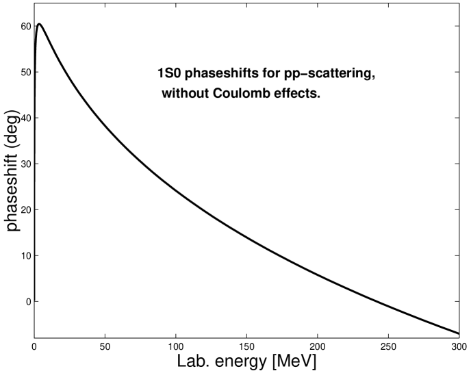
Figure 11: Phaseshift for proton-proton scattering in the ${}^{1}S_{0}$ channel. Coulomb effects are not included in the calculations.

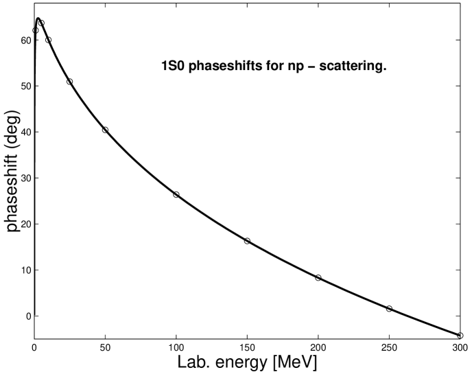
Figure 12: Phaseshift for neutron-proton scattering in the ${}^{1}S_{0}$ channel. Calculation by the contour deformation method is given by the solid line. Circles are calculations given in Ref. machleidt .

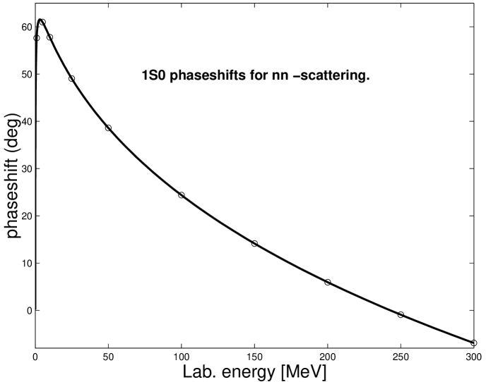
Figure 13: Phaseshift for neutron-proton scattering in the ${}^{1}S_{0}$ channel. Calculation by the contour deformation method is given by the solid line. Circles are calculations given in Ref. machleidt .

VI Conclusions and perspectives

A generalized contour deformation method in momentum space has been presented. The deformation of the integration contour is generalized to rotation followed by translation in the complex $k$-plane. This generalization makes it possible to handle both dilation and non-dilation invariant potentials. We have shown this to be a powerful procedure for studying resonances and virtual states in two-body systems. The method has also been successfully applied to the calculation of the full off-shell $t$-matrix. The aim of this work has been to establish the formalism for the free scattering case, basing the analysis on schematic and realistic nucleon-nucleon interactions. Work on extension to few-body Borromean halo systems zhukov with more than two constituents, is in progress.

The exposed formalism allows for stable numerical calculations of bound states, resonances and virtual states, in addition to yielding a fully complex on-shell and off-shell scattering matrix, starting with a realistic nucleon-nucleon interaction.

This allows for several interesting applications and extensions. As is well-known, one of the major challenges in the microscopic description of weakly bound nuclei is a proper treatment of both the many-body correlations and the continuum of positive energies and decay channels. Such nuclei pose a tough challenge on traditional nuclear structure methods, based essentially on the derivation of effective interactions and the nuclear shell-model, see for example Ref. mhj95 for a review. In the traditional approaches only bound states typically enter the determination of an effective interaction, be it either based upon various many-body schemes or more phenomenologically inspired approaches. Coupled with large-scale shell model studies, several properties of stable nuclei are well reproduced. However, weakly bound nuclei may have a strong coupling to unbound states, either resonances or virtual states, as described in for example Refs. witek1 ; witek2 ; roberto . This implies in turn that an effective interaction should reflect such couplings with the continuum, i.e., a consistent many-body scheme should include bound states, resonances and virtual states as well.

The present approach may allow for such a scheme. The simplest extension is to consider in-medium scattering of two nucleons in e.g., infinite nuclear matter or neutron star matter, as done by Dickhoff and et al. dickhoff1998 or Schulze et al. hansjosef . This is easily accomplished by inserting an exclusion operator $Q$ in Eq. (12) for the Green’s operator. This exclusion operator can be constructed so as to prevent scattering into occupied states. Typically, one can then generate selected hole-hole, particle-hole and particle-particle intermediate state correlations that reflect a given nuclear medium. Combined with a self-consistent determination of the single-particle energies it is then possible to derive various classes of diagrams at the two-body level. Such work is in progress, based on the present method and the exact definition of the exclusion operator $Q$ by Suzuki et al. kenyj_rioyj .

References

- (1) R. G. Newton Scattering Theory of Waves and Particles (Springer-Verlag, New York, 1966,1982).
- (2) V. I. Kukulin, V. M. Krasnopol’sky, and J. Horek, Theory of Resonances (Kluwer Academic publishers 1989).
- (3) I. R. Afnan, Aust. J. Phys. 44 , 201 (1991).
- (4) J. Aguilar and J. M. Combes, Commun. Math. Phys. 22, 269 (1971).
- (5) E. Balslev and J. M. Combes, Commun. Math. Phys. 22, 280 (1971).
- (6) N. Moiseyev, Phys. Rep. 302, 211 (1998).
- (7) A. Csoto, Phys. Rev. C 49, 2244 (1994).
- (8) E. Garrido, D. V. Fedorov, and A. S. Jensen, Nucl. Phys. A 708, 277 (2002).
- (9) I. Raskinyte, Resonances in few-body systems, PhD Thesis University of Bergen 2002.
- (10) D. Brayshaw, Phys. Rev. 176 , 1855 (1968).
- (11) J. Nuttall and H. L. Cohen, Phys. Rev. 188, 1542 (1969).
- (12) A. T. Stelbovics, Nucl. Phys. A 288, 461 (1978).
- (13) T. Berggren, Nucl. Phys. A 109, 265 (1968)
- (14) P. Lind, Phys. Rev. C 47, 1903 (1993)
- (15) J. Nuttall, J. Math. Phys. 8, 873 (1967).
- (16) G. Tiktopoulos, Phys. Rev. 136, 275 (1964).
- (17) S. Aoyama, Phys. Rev. Lett. 89, 052501 (2002).
- (18) B. C. Pearce and I. R. Afnan, Phys. Rev. C 30, 2022 (1984).
- (19) K. Yamaguchi, Phys. Rev. 95, 1628 (1954).
- (20) R. A. Malfliet and J. A. Tjon, Nucl. Phys. A 127, 161 (1969).
- (21) R. Machleidt, Phys. Rev. C 63, 024001 (2001).
- (22) R. Id Betan, R. J. Liotta, N. Sandulescu, and T. Vertse, Phys. Rev. C 67, 014322 (2003).
- (23) L. Brown, D. Fivel, B. W. Lee, and R. Sawyer, Ann. of Phys. 23, 167 (1963).
- (24) Ch. Elster, J. H. Thomas, and W. Glöckle, Few-Body Systems 24, 55 (1998).
- (25) M. V. Zhukov, B. V. Danilin, D. V. Fedorov, J. M. Bang, I. J. Thompson, and J. S. Vaagen, Phys. Rep. 231, 151 (1993).
- (26) M. Hjorth-Jensen, T. T. S. Kuo, and E. Osnes, Phys. Rep. 261, 125 (1995).
- (27) N. Michel, W. Nazarewicz, M. Płoszajczak, and K. Bennaceur, Phys. Rev. Lett. 89, 042502 (2002).
- (28) N. Michel, W. Nazarewicz, M. Płoszajczak, and J. Okołowicz, nucl-th/0302060.
- (29) R. Id Betan, R. J. Liotta, N. Sandulescu, and T. Vertse, Phys. Rev. Lett. 89, 042501 (2002).
- (30) W. H. Dickhoff, Phys. Rev. C 58, 2807 (1998); W. H. Dickhoff, C. C. Gearhart, E. P. Roth, A. Polls, and A. Ramos, Phys. Rev. C 60, 064319 (1999).
- (31) H.-J. Schulze, A. Schnell, G. Röpke, and U. Lombardo, Phys. Rev. C 55, 3006 (1997).
- (32) K. Suzuki, R. Okamoto, M. Kohno, and S. Nagata, Nucl. Phys. A 665, 92 (2000).