FZJ-IKP-TH-2003-4

An analysis of the reaction $pp\rightarrow pp\eta$ near threshold

Abstract

It is shown that most of the available data on the $pp\rightarrow pp\eta$ reaction, including the invariant mass distributions in the $pp\rightarrow pp\eta$ reaction recently measured at COSY, can be understood in terms of the partial-wave amplitudes involving final $pp$ $S$ and $P$ states and the $\eta$ meson $s$-wave. This finding, together with the fact that results within a meson–exchange model are especially sensitive to the details of the excitation mechanism of the $S_{11}(1535)$ resonance, demonstrates the possibility of investigating the properties of this resonance in $NN$ collisions. The spin correlation function $C_{xx}$ is shown to disentangle the $S$- and $P$-wave contributions. It is also argued that spin correlations may be used to help constrain the contributions of the amplitudes corresponding to the final $pp$ ${}^{3}P_{0}$ and ${}^{3}P_{2}$ states.

The primary motivations for studying the production of mesons off nucleons and nuclei are to investigate the structure and properties of the nucleon resonances and to learn about hadron dynamics at short range. As far as hadron-induced reactions are concerned, and specifically nucleon-nucleon ($NN$) collisions, there is already a wealth of information on the production of the lightest meson, the pion. In particular, there now exists a fairly accurate and complete set of data, especially for $\pi^{o}$ production in the near-threshold energy region Meyer , which should allow for a partial wave analysis. The $\eta$ meson, which is the next lightest non-strange meson in the meson mass spectrum, has also been the subject of considerable interest. A peculiar feature of this meson is that it couples strongly to the $S_{11}(1535)$ nucleon resonance, which offers a unique opportunity for investigating the properties of this resonance. Unfortunately, the experimental information on $\eta$ production in $NN$ collisions EXP ; Calena ; Calend ; Winter ; Roderburg ; Moskal is much less complete than for pion production and is not yet sufficient for a model-independent partial-wave analysis. However, the available data base has greatly expanded recently thanks to measurements by the TOF and COSY-11 collaborations at COSY Roderburg ; Moskal that provided, not only $\eta$ and proton angular distributions, but also $pp$ and $p\eta$ invariant mass distributions for the reaction $pp\rightarrow pp\eta$. These new data, together with the earlier measurements EXP ; Calena ; Calend , open the possibility for investigating this reaction in much more detail than could be done previously.

A general feature of meson production in $NN$ collisions is that the energy dependence of the total cross section in the near-threshold region is basically dictated by the available phase space plus the $NN$ final state interaction (FSI) in $S$ states. The effect of the strong $NN$ FSI also shows up in the corresponding $NN$ invariant mass spectrum as a peak close to the threshold value of the invariant mass, $m_{NN}=2m_{N}$, where $m_{N}$ denotes the nucleon mass. Surprisingly, the recently measured $pp$ invariant mass distribution in the reaction $pp\rightarrow pp\eta$ Roderburg ; Moskal at excess energies of $Q=15$ and $41$ MeV shows, in addition to a peak very close to the threshold, a broad bump at higher values of $m_{pp}$ (see Fig. 1). While the peak can easily be understood as arising from the strong $pp$ FSI in the ${}^{1}S_{0}$ state as mentioned above, it is not trivial to explain the origin of the bump at higher $m_{pp}$.

The purpose of the present work is to analyze this seemingly peculiar feature exhibited by the $pp$ invariant mass distribution. Thereby we will show that the available data on $pp\rightarrow pp\eta$, including the invariant mass distribution, can essentially be understood in terms of $S$- and $P$-wave amplitudes. This result suggests that the properties of the $S_{11}(1535)$ nucleon resonance can be studied here in terms of only a few partial-wave amplitudes. We start by considering the possible partial-wave states in $pp\rightarrow pp\eta$ near the threshold notation . First, in this reaction, the $\eta$ meson is dominantly produced through the excitation and de-excitation of the $S_{11}(1535)$ resonance. Therefore we expect that the $\eta$ meson should be produced mainly in the $s$-wave. Of course, this is strictly true only in the rest frame of the resonance and not necessarily in the overall c.m. frame of the system. However, near threshold, this should not make a significant difference. In fact, the observed $\eta$ angular distribution in the overall c.m. frame Roderburg is practically isotropic. In addition, the very first analyzing power measurement in $pp\rightarrow pp\eta$ by the COSY-11 group Winter yielded rather small values. Indeed this observable is basically consistent with zero, given the relatively large uncertainties involved, and therefore consistent with pure $s$-wave contributions. As long as we restrict ourselves to an $\eta$ meson in the $s$-wave and final $NN$ state to the $S$ and $P$ waves, we have only three partial-wave amplitudes that can contribute to this reaction notation : ${}^{3}P_{0}\rightarrow\,^{1}S_{0}s$, ${}^{1}S_{0}\rightarrow\,^{3}P_{0}s$ and ${}^{1}D_{2}\rightarrow\,^{3}P_{2}s$. Among these, we would naively expect that the ${}^{3}P_{0}\rightarrow\,^{1}S_{0}s$ is the only relevant contribution near threshold. However, as mentioned above, the contribution of the $S$–wave alone is unable to explain the observed bump in the $pp$ invariant mass distribution.

One plausible explanation may be attributed to effects from the $\eta N$ FSI. Indeed there are already strong indications from the total production cross sections that the $\eta N$ FSI may play an important role in the reaction $NN\to NN\eta$ near threshold. For both $pp$ and $pn$ induced $\eta$ productions one has observed that there is an enhancement of the production cross sections for very small excess energies that cannot be explained by the $NN$ FSI effects alone Calend ; Moskal0 . However, those effects seem to be confined to an excess energy range of up to at most 20 MeV from the threshold. Thus, one would expect that the $\eta N$ FSI effects should have an influence on the invariant mass spectrum measured at the lower energy of $Q$ = 15 MeV. It is, however, unlikely that such effects should still be so important at $Q$ = 41 MeV. A proper inclusion of the $\eta N$ FSI calls for solving the Faddeev equation in the three-particle continuum which is technically very involved. A rough estimate suggests that a rather strong $\eta N$ interaction would be needed to reproduce the data at the higher energy Baru_pc , which is difficult to be reconciled with other information about the $\eta N$ interaction. Therefore, we seek an alternative explanation based largely on the observation that the shape of the bump can be reproduced by folding $p^{\prime 2}$ with the available phase space. Here, $p^{\prime}$ denotes the relative momentum in the final $pp$ system. This suggests to us, that the bump seen in the experiment could be simply caused by the $pp$ $P$-wave in the final state. Admittedly, the measured final proton angular distribution in the overall c.m. frame is nearly isotropic Roderburg , which could be seen as an evidence against large $P$-wave and higher partial wave contributions. However, as we shall show below, there is no principal contradiction between a nearly isotropic proton distribution and a significant $P$-wave fraction in the invariant mass spectrum.

Let us now make some general remarks about the structure of the reaction amplitude for $pp\rightarrow pp\eta$. In what follows, we shall assume that the $\eta$ is in an $s$ wave relative to the (final) $pp$ system and that the final protons are in a relative $S$ and/or $P$ state. Since the $\eta$ meson is an isoscalar pseudoscalar particle, it follows immediately that the orbital angular momentum of the $pp$ system has to change in the transition from the initial to the final state and consequently, due to the Pauli principle, the total spin also has to change. Thus, the most general form of the reaction matrix (involving even angular momenta of $\eta$) can be written as

$${\cal M}=\left(\vec{A}P_{S^{\prime}=0}-\vec{B}P_{S^{\prime}=1}\right)\cdot{\frac{1}{2}}\left(\vec{\sigma}_{1}-\vec{\sigma}_{2}\right)\ ,$$ (1)

where $P_{S^{\prime}=0,1}$ stands for the total spin singlet and triplet projection operator as the total spin of the two protons in the final state, $S^{\prime}$, takes the value $S^{\prime}=0$ and $S^{\prime}=1$, respectively. $\vec{\sigma}_{i}$ denotes the Pauli spin matrix acting on each of the two interacting protons, $i=1$ and $2$. In terms of the Pauli spin matrices, we have $P_{S^{\prime}=0}=(1-\vec{\sigma}_{1}\cdot\vec{\sigma}_{2})/4$ and $P_{S^{\prime}=1}=(3+\vec{\sigma}_{1}\cdot\vec{\sigma}_{2})/4$. We, then, may write, $P_{S^{\prime}}(\vec{\sigma}_{1}-\vec{\sigma}_{2})/2=\left[(\vec{\sigma}_{1}-\vec{\sigma}_{2})-(-)^{S^{\prime}}i(\vec{\sigma}_{1}\times\vec{\sigma}_{2})\right]/4$, which, up to an irrelevant phase, is identical to the structure given in Ref. Bernard . The vectors $\vec{A}$ and $\vec{B}$ in Eq. (1) may be constructed from the momentum vectors available in the system, e.g., the relative momenta of the two protons in the initial state $\vec{p}$ and in the final state $\vec{p}\,^{\prime}$. Since we restrict ourselves to $S$ and $P$ waves for the outgoing $pp$ system we may write

$$\vec{A}=\alpha\hat{p}\ ,\ \ \ \vec{B}=\beta\vec{p}\,^{\prime}+\gamma(\vec{p}\,^{\prime}-3\hat{p}(\hat{p}\cdot\vec{p}\,^{\prime}))\ .$$ (2)

Here the amplitudes $\alpha$, $\beta$, and $\gamma$ correspond to the transitions ${}^{3}P_{0}\rightarrow\,^{1}S_{0}s$, ${}^{1}S_{0}\rightarrow\,^{3}P_{0}s$, and ${}^{1}D_{2}\rightarrow\,^{3}P_{2}s$, respectively. Note that we pulled out the linear momentum dependence, characteristic of $P$–waves, from the corresponding partial-wave amplitudes. The amplitude $\alpha$ has a strong dependence on the relative energy of the $pp$ system in the final state reflecting the strong $pp$ FSI in the ${}^{1}S_{0}$ state. The amplitudes $\beta$ and $\gamma$ also depend on the relative energy of the $pp$ system in the final state; however, their energy dependence is much weaker than that of $\alpha$ due to the much weaker $pp$ FSI in the ${}^{3}P_{0}$ and ${}^{3}P_{2}$ states as compared to the ${}^{1}S_{0}$ state.

From Eq. (1) explicit expressions for any observable follow directly. E.g., we find

$$\frac{d\sigma}{d\Omega}\phantom{A_{j}} = |\vec{A}|^{2}+|\vec{B}|^{2}\ ,$$

$$\frac{d\sigma}{d\Omega}A_{j} = i(\vec{A}\,^{*}\times\vec{A})_{j}\ ,$$

$$\frac{d\sigma}{d\Omega}C_{ij} = \delta_{ij}\left(|\vec{A}|^{2}-|\vec{B}|^{2}\right)-2\mbox{Re}\left(A^{*}_{i}A_{j}\right)\ ,$$ (3)

where $A_{j}$ denotes the analyzing power and $C_{ij}$ the spin correlation function. Inserting the expressions of Eq. (2) into Eq. (3) we get

$$\frac{d\sigma}{d\Omega}\phantom{A_{j}} = |\alpha|^{2}+p^{\prime}\,{}^{2}\left[|\beta+\gamma|^{2}+3x^{2}(|\gamma|^{2}-2\mbox{Re}(\beta\gamma^{*}))\right]\ ,$$

$$\frac{d\sigma}{d\Omega}A_{j} = 0\ ,$$

$$\frac{d\sigma}{d\Omega}C_{xx} = |\alpha|^{2}-p^{\prime}\,{}^{2}\left[|\beta+\gamma|^{2}+3x^{2}(|\gamma|^{2}-2\mbox{Re}(\beta\gamma^{*}))\right]\ ,$$ (4)

where we introduced $p^{\prime}x=\vec{p}\,^{\prime}\cdot\hat{p}$. We note that partial-wave amplitudes with even and odd final $pp$ relative orbital angular momenta cannot interfere with each other due to the Pauli principle.

Let us recall at this stage that the proton angular distribution seen in the experiment is isotropic Roderburg . From the above equations we can see immediately that there are two possible scenarios for achieving such an isotropic distribution in the presence of significant $pp$ $P$–wave contributions, namely

• Dominant contributions from the transitions ${}^{3}P_{0}\rightarrow\ ^{1}S_{0}s$ and ${}^{1}S_{0}\rightarrow\ ^{3}P_{0}s$, but negligible contributions from ${}^{1}D_{2}\rightarrow\ ^{3}P_{2}s$ ($\gamma\approx 0$).

• Contributions from all three transitions, ${}^{3}P_{0}\rightarrow\ ^{1}S_{0}s$, ${}^{1}S_{0}\rightarrow\ ^{3}P_{0}s$ and ${}^{1}D_{2}\rightarrow\ ^{3}P_{2}s$, where the latter two interfere destructively ($|\gamma|^{2}\approx 2{\rm Re}(\beta\gamma^{*})$).

Obviously, the observables given in Eq. (4) do not allow one to distinguish between the two scenarios and, consequently, there is no model independent way to extract the two $pp$ $P$-wave amplitude contributions ($\beta$ and $\gamma$) from these observables. To do that, one would need observables depending also on the spin of the final $pp$ state, such as spin transfer coefficients. Note, however, that the combination $d\sigma/d\Omega\,(C_{xx}+1)$ depends only on the amplitude $\alpha$. Hence, a measurement of this observable would determine, in a model independent way, the $pp$ $S$–wave contribution ($\alpha$) in the final state. Similarly, a measurement of $d\sigma/d\Omega\,(C_{xx}-1)$ would confirm the presence of $pp$ $P$–waves in the final state. It should also be stressed that $C_{xx}$ by itself is already very interesting. Here the two angular independent terms (first two terms in the last equation of (4)) have opposite signs and thus tend to cancel each other. Consequently, this observable should be rather sensitive to the angular dependent term.

We now turn our attention to the results of a model for $pp\rightarrow pp\eta$. In Ref. Nak1 we have presented a relativistic meson-exchange model for $\eta$ production in $NN$ collisions. It treats $\eta$ production in the Distorted Wave Born Approximation and includes both the $NN$ FSI and initial state interaction (ISI), the latter through the approximate procedure proposed in Ref. ours . While this model yields a satisfactory description of the near-threshold cross section data (for $pp\to pp\eta$ and for $pn\to pn\eta$) it fails to reproduce the recently measured invariant mass distributions. It should be stressed that the main objective of the present model calculation is not to achieve an accurate description of the existing data but rather to verify whether the model of Ref. Nak1 can be modified so as to comply with the major features exhibited by the new data Roderburg ; Moskal as discussed above.

In the development of a variant of the model Nak1 we have restricted ourselves to modifications of the $vNN^{*}$ vertex and the mixing parameter $\lambda$ in the $\pi NN^{*}$ and $\eta NN^{*}$ vertices. Here, $v$ stands for either the $\rho$- or $\omega$-meson and $N^{*}$ is the $S_{11}(1535)$ resonance. We also use the Paris $NN$ T-matrix Lacomb as the $pp$ FSI; the Coulomb interaction is fully accounted for as described in Ref. Nak2 . Everything else was kept unchanged. In contrast to Ref. Nak1 , in the present work we have chosen a more general gauge invariant Lagrangian Riska for the $vNN^{*}$ coupling

$${\cal L}^{(\pm)}_{\omega NN^{*}}(x) = \left(\frac{g_{\omega NN^{*}}}{m_{N^{*}}+m_{N}}\right)\bar{\psi}_{N^{*}}(x)\gamma_{5}\left\{\left[\gamma_{\mu}\frac{\partial^{2}}{m_{N^{*}}+m_{N}}-i\partial_{\mu}+\kappa_{\omega}\sigma_{\mu\nu}\partial^{\nu}\right]\omega^{\mu}(x)\right\}\psi_{N}(x)$$ (5a)

$$+ h.c.\ ,$$

$${\cal L}^{(\pm)}_{\rho NN^{*}}(x) = \left(\frac{g_{\rho NN^{*}}}{m_{N^{*}}+m_{N}}\right)\bar{\psi}_{N^{*}}(x)\gamma_{5}\left\{\left[\gamma_{\mu}\frac{\partial^{2}}{m_{N^{*}}+m_{N}}-i\partial_{\mu}+\kappa_{\rho}\sigma_{\mu\nu}\partial^{\nu}\right]\vec{\tau}\cdot\vec{\rho}^{\,\mu}(x)\right\}\psi_{N}(x)$$ (5b)

$$+ h.c.\ ,$$

where $\omega^{\mu}(x)$, $\vec{\rho}^{\,\mu}(x)$, $\psi_{N}(x)$ and $\psi_{N^{*}}(x)$ denote the $\omega$, $\rho$, nucleon and spin-1/2 $N^{*}$ (=$S_{11}(1535)$) resonance fields, respectively. $m_{N^{*}}$ denotes the mass of the nucleon resonance. The coupling constants $g_{vNN^{*}}$ and $\kappa_{v}$ were considered to be free parameters in the calculation and have been adjusted to reproduce (globally) the available data, including the $pp\eta$ and $pn\eta$ total cross sections. The $\gamma_{5}\gamma_{\mu}$ coupling at the $vNN^{*}$ vertex was necessary to achieve a reasonable fit to the data. The values obtained are: $g_{\rho NN^{*}}/(m_{N}^{*}+m_{N})$ = 9.5 [$fm$], $\kappa_{\rho}$ = -5.3 and $g_{\omega NN^{*}}/(m_{N}^{*}+m_{N})$ = 6.0 [$fm$], $\kappa_{\omega}$ = 3.8. In addition to the $vNN^{*}$ vertex given above, we have also chosen the pseudoscalar-pseudovector mixing parameter to be $\lambda=0.7$ at the $\pi NN^{*}$ and $\eta NN^{*}$ vertices Nak1 . All other parameter values are the same as given in Ref. Nak1 corresponding to the case of pseudoscalar meson dominance. We refer to Ref. Nak1 for further details of the model.

Results for the $pp$ invariant mass distribution based on different partial wave contributions are shown in Fig. 1 together with the recent data at the excess energies of $Q=15$ Roderburg ; Moskal and $41$ MeV Roderburg . The full results are denoted by solid curves. Hereafter, these correspond to the calculations performed using the plane-wave basis without a partial wave decomposition and, as such, they include all partial waves. As is evident from the dashed curves, the observed peak in the region $m_{pp}^{2}\sim(2m_{N})^{2}$ is due to the strong $pp$ FSI in the ${}^{1}S_{0}$ state. The observed bump in the higher $m_{pp}$ region is largely due to the ${}^{3}P_{0}s$ final state (dash-dotted curves). The contribution from the ${}^{3}P_{2}s$ state (dotted curves) is very small. Contributions from other partial-wave states (mainly ${}^{3}P_{2},^{3}F_{2}\rightarrow^{1}S_{0}d$) are relatively small at $Q=41$ MeV and practically negligible at $Q=15$ MeV. Thus, the present model is in line with the scenario (1) discussed above. Overall, the shape of the $pp$ invariant mass distribution exhibited by the data is nicely reproduced. However, the model tends to overestimate the data close to the maximum value of $m_{pp}^{2}$ at $Q=41$ MeV. In principle, this discrepancy might be due to the $p\eta$ FSI which is not explicitly accounted for in our model Nak1 . However, in order to reduce the predicted value, one needs a repulsive $p\eta$ FSI which seems to be in contradiction with all other evidence of $p\eta$ FSI effects in meson production Moskal0 ; xxx . Moreover, no such discrepancy is seen at $Q=15$ MeV where the effect of the $p\eta$ FSI should be even larger. Further investigation is required to resolve this issue.

It is important to note that the relative strength of the different partial-wave states depends crucially on the details of the model, and that means, specifically, on the excitation mechanism of the $S_{11}(1535)$ resonance in the present case. In fact, the measured $pp$ invariant mass distributions can be described with the same quality as shown in Fig. 1 with the ${}^{3}P_{2}s$ state contribution dominating over the ${}^{3}P_{0}s$ state contribution. Such a scenario can easily be achieved in our model by a proper adjustment of the coupling constants at the $vNN^{*}$ vertex appearing in the underlying Lagrangians (Eq. (5)). However, the resulting proton angular distributions are then much more pronounced and, consequently, in disagreement with the experimental evidence Roderburg .

Although significant $pp$ $P$-waves in the final state seem to be necessary for reproducing the $pp$ invariant mass distribution, it is important to note that the energy dependence of the total cross section near the threshold energy region is basically reproduced by the $pp$ FSI in the ${}^{1}S_{0}$ state folded with the phase space. E.g., the model developed by V. Baru et al. Baru reproduces nicely the energy dependence of the total cross section from threshold up to $Q\sim 50$ MeV with $S$–wave contributions alone. Results of the present model for the total cross section are shown in Fig. 2. Comparing the curves for the ${}^{1}S_{0}s$ (long-dashed) and ${}^{1}S_{0}s+^{3}P_{0}s$ (dash-dotted) partial waves, one realizes that the onset of the ${}^{3}P_{0}s$ final state occurs at a fairly low excess energy and that its contribution becomes increasingly important with increasing energy. This feature is a direct consequence of the requirement of reproducing the $pp$ invariant mass distribution. However, as a result, the model now underpredicts significantly the data for energies close to threshold. The thin dashed curve corresponds to the ${}^{1}S_{0}s$ contribution multiplied by an arbitrary factor of 3. This clearly shows that the total cross section data in the low energy region favor a larger contribution of the ${}^{1}S_{0}s$ final state than is predicted by our model. Whether one is able to reconcile these seemingly contradictory properties within a consistent theoretical model remains to be seen. In any case, one should keep in mind that the $\eta N$ FSI, which is not included in the present model calculation, should enhance the $\eta$ $s$-wave contribution near threshold to some degree gar .

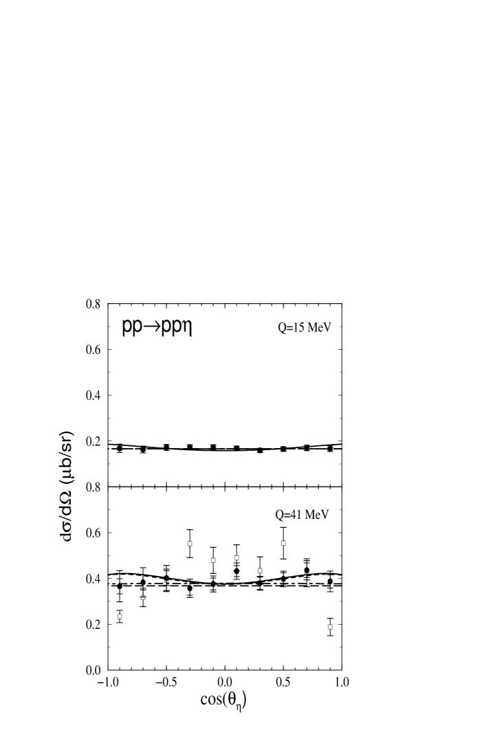
Figure 3: Angular distribution of the emitted $\eta$ meson in the c.m. frame of the total system at an excess energy of $Q=15$ MeV (upper panel) and $Q=41$ MeV (lower panel). The dashed (dash-dotted) curves correspond to the $\eta$ meson $s$-wave ($s+p$-wave) contribution. The dotted curves correspond to the $s+p+d$-wave contributions which are practically indistinguishable from the corresponding full results represented by solid curves. The data are from Refs. Calena ; Roderburg .

Fig. 3 shows the differential cross sections as a function of the $\eta$ emission angle in the overall c.m. frame for two excess energies. The data from Ref. Roderburg are basically isotropic, indicating a dominant $\eta$ $s$-wave contribution. The theoretical results are normalized to the total cross section (obtained by integrating the differential cross section data) in order to facilitate a proper comparison of their angular dependence with the experiment. At $Q=15$ MeV the normalization factor is about 2.7, while at $Q=41$ MeV, it is about 0.9. The dashed curves correspond to the $s$-wave contribution, the dash-dotted curves to the $s+p$ waves, and the dotted curves to the $s+p+d$ waves. The last are practically indistinguishable from the corresponding full results which are denoted by the solid lines. As expected after the discussion above, the angular distribution is given primarily by the $s$-wave contribution, with a small contribution from higher partial waves provided mainly by the $d$-wave.

In Fig. 4, the proton angular distributions in the overall c.m. frame are shown together with the data from Ref. Roderburg . Here again the model predictions are normalized to the data using the same factor mentioned above. Evidently, at $Q=15$ MeV the result is isotropic; it is dominated by the ${}^{1}S_{0}s$ (dashed curve) state followed by the ${}^{3}P_{0}s$ (dash-dotted curve) state. Contributions from other partial waves are practically negligible. At $Q=41$ MeV there is a small contribution from the ${}^{3}P_{2}s$ (dotted curve). Obviously, the destructive interference with the ${}^{3}P_{0}s$ state canceling the angular dependence (see Eqs.(4)) is incomplete resulting in a noticeable angular dependence which, however, is still compatible with the experiment. The difference between the dotted and solid curves is due to a small contribution from the ${}^{3}P_{2}\rightarrow^{1}D_{2}s$ plus ${}^{3}P_{2},^{3}F_{2}\rightarrow^{1}S_{0}d$ amplitudes.

Fig. 5 shows the prediction for the analyzing power as a function of the $\eta$ emission angle in the overall c.m. frame. The data are from Ref. Winter . The dashed curves correspond to the $\eta$ $s+p$ wave contributions while the dash-dotted curves to the $s+p+d$ waves. The solid lines are the full results. We note that the $s$-wave contribution alone yields $A_{y}\equiv 0$ (see Eqs.(4)), so that any non-vanishing result must necessarily involve higher partial waves. Furthermore, judging from the shape exhibited by the analyzing power, the present model yields a vector meson dominance over the pseudoscalar meson in the excitation mechanism of the $S_{11}(1535)$ resonance as discussed in Ref. Nak1 . Although the data indicate some contribution from partial waves higher than the $s$-wave, they are not sufficiently accurate to make a definitive statement as to the size of their contribution.

In Fig. 6 we present predictions for the spin correlation function $C_{xx}$ at $Q=41$ MeV as a function of the proton angle in the overall c.m. frame. As can be seen from Eq. (4), the ${}^{3}P_{0}\rightarrow\,^{1}S_{0}s$ partial wave alone leads to a constant value of $C_{xx}=1$. Adding the ${}^{1}S_{0}\rightarrow\,^{3}P_{0}s$ contribution (dashed curve) yields a small value of $C_{xx}\sim-0.3$. Including also the ${}^{1}D_{2}\rightarrow\,^{3}P_{2}s$ contribution one obtains the result represented by the dotted line. (In this context note that the ${}^{1}S_{0}\rightarrow\,^{3}P_{0}s$ as well as the ${}^{1}D_{2}\rightarrow\,^{3}P_{2}s$ contributions alone would give rise to $C_{xx}=-1$, cf. Eq. (4)). Other partial-wave contributions do not change $C_{xx}$ qualitatively as is evident from the full result (solid curve). Thus, in our model, the cancellation of the $|\alpha|^{2}$ term and the $|\beta+\gamma|^{2}$ in Eqs. (4) is almost complete! This strongly enhances the relative importance of the angular dependent term in $C_{xx}$. Note that $C_{xx}=C_{yy}$ for all of the three partial-wave contributions discussed explicitly above (c.f. Eqs. (3)).

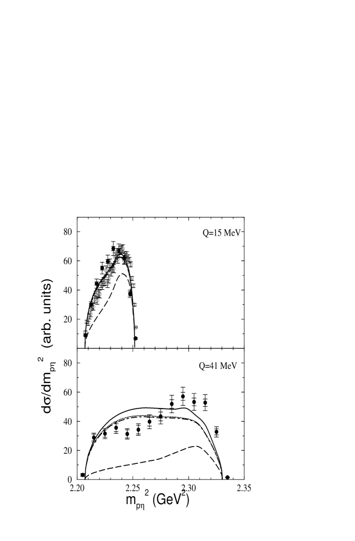
Figure 7: Same as Fig. 1 but for the $p\eta$ invariant mass distribution. The data from Ref. Moskal (open circle) have been normalized by an arbitrary factor of 0.66 in order to facilitate the comparison of the shape with the data from Ref. Roderburg and the present model prediction.

In Fig. 7 predictions for the $p\eta$ invariant mass distribution are shown together with the data Roderburg . Again, the dominant contributions are from the ${}^{1}S_{0}s$ (dashed curves) and ${}^{3}P_{0}s$ (dot-dashed curves) final states; the contribution from the ${}^{3}P_{2}s$ state (dotted curves) is negligible. At $Q=41$ MeV one sees also some effects from other partial-wave states arising mainly from the ${}^{3}P_{2},^{3}F_{2}\rightarrow^{1}S_{0}d$ amplitude. The overall shape of the measured invariant mass distribution is reproduced. The observed discrepancies in the details, especially at $Q=41$ MeV, are not easy to understand in view of the nice agreement between calculated and measured $pp$ invariant mass distributions.

Summarizing our results, we have shown that the currently available data on $\eta$ production in $pp$ collisions near the threshold energy can be largely understood in terms of a few $S$- and $P$-wave amplitudes. For a completely model-independent extraction of the relevant amplitudes, however, observables independent of those presently available are required. In this connection, the spin correlation function, either $C_{yy}$ or $C_{xx}$, is suited to further constrain the ${}^{3}P_{0}s$ and ${}^{3}P_{2}s$ final state contributions. In any case, the final $pp$ $P$-wave contribution is crucial for explaining the measured invariant $pp$ mass distribution, especially, at $Q=41MeV$. Our model calculations show that, the dominant amplitudes are ${}^{3}P_{0}\rightarrow\ ^{1}S_{0}s$ and ${}^{1}S_{0}\rightarrow\ ^{3}P_{0}s$. It should be stressed that in order to quantify the role of the $\eta N$ interaction in $pp\to pp\eta$ it is important to first understand the role of higher $NN$ partial waves.

Finally, we note that the present work illustrates the possibility of using meson production processes in $NN$ collisions to study the properties of nucleon resonances in terms of a few partial-wave amplitudes. In particular, the present model prediction for the relevant partial-wave amplitudes depends very sensitively on the details of the model and especially to the excitation mechanism of the $S_{11}(1535)$ resonance. This offers an excellent opportunity to study some of the properties of the $S_{11}(1535)$ resonance using the $\eta$ meson production reaction in $NN$ collisions which would not be possible to investigate in more basic reactions such as $\gamma+N\rightarrow\eta+N$ and $M+N\rightarrow\eta+N$.

Acknowledgement: The authors would like to acknowledge many fruitful discussions with V. Baru, and W. G. Love. The authors also thank W. G. Love for a careful reading of this manuscript. This work is supported by COSY grant No 41445282(COSY-58).

Figure 1: Final $pp$ invariant mass distribution in $pp\rightarrow pp\eta$ as a function of invariant mass squared, $m_{pp}^{2}$, at an excess energy of $Q=15$ MeV (upper panel) and $Q=41$ MeV (lower panel). The dashed (dash-dotted) curves correspond to the ${}^{1}S_{0}s$ (${}^{1}S_{0}s+^{3}P_{0}s$) final state contribution. The dotted curves correspond to ${}^{1}S_{0}s+^{3}P_{0}s+^{3}P_{2}s$; its is indistinguishable from the solid curve in the upper panel. The solid curves are the full results. The data are from Ref. Roderburg (filled circle) and Ref. Moskal (open circle). The latter have been normalized by an arbitrary factor of 0.66 in order to facilitate the comparison of the shape with the former data and the present model prediction.

Figure 2: Total cross section for the reaction $pp\rightarrow pp\eta$ as a function of the excess energy $Q$. The solid curves represent the full results. The dashed (dash-dotted) curve corresponds to the ${}^{1}S_{0}s$ (${}^{1}S_{0}s+^{3}P_{0}s$) final-state contribution and the dotted curve to the ${}^{1}S_{0}s+^{3}P_{0}s+^{3}P_{2}s$ contribution. The thin dashed curve is the ${}^{1}S_{0}s$ contribution multiplied by an arbitrary factor of 3. The data are from Ref. EXP .

Figure 4: Angular distribution of the proton in the final state in the c.m. frame of the total system at an excess energy of $Q=15$ MeV (upper panel) and $Q=41$ MeV (lower panel). The dashed (dash-dotted) curves correspond to the ${}^{1}S_{0}s$ (${}^{1}S_{0}s+^{3}P_{0}s$) final-state contribution. The dotted curve corresponds to the ${}^{1}S_{0}s+^{3}P_{0}s+^{3}P_{2}s$ contribution and the solid curve represents the full result. The data are from Ref. Roderburg .

Figure 5: Analyzing power for the reaction $pp\rightarrow pp\eta$ as a function of $\eta$ emission angle in the c.m. frame of the total system at an excess energy of $Q=15\ MeV$ (upper panel) and $Q=41\ MeV$ (lower panel). The dashed (dash-dotted) curves correspond to the partial waves contributions with $l^{\prime}\leq 1$ ($l^{\prime}\leq 2$). The solid curves represent the full results. The data are from Ref. Winter .

Figure 6: Predicted spin correlation function $C_{xx}$ for the reaction $pp\rightarrow pp\eta$ as a function of final proton angle in the overall c.m. frame at an excess energy of $Q=41$ MeV. The dash (dash-dotted) curve corresponds to the ${}^{1}S_{0}s$ (${}^{1}S_{0}s+^{3}P_{0}s$) final state contribution. The dotted curve corresponds to the ${}^{1}S_{0}s+^{3}P_{0}s+^{3}P_{2}s$ contribution and the solid curve represents the full result.

References

- (1) H. O. Meyer et al., Phys. Rev. C63 064002 (2001).
- (2) E. Chiavassa et al., Phys. Lett. B322 270 (1994); H. Calén et al., Phys. Rev. Lett. 79 2642 (1997); F. Hibou et al., Phys. Lett. B438 41 (1998); J. Smyrski et al., Phys. Lett. B474 180 (2000); B. Tatischeff et al., Phys. Rev. C62 054001 (2000); H. Calén et al., Phys. Rev. C58 2667 (1998).
- (3) H. Calén et al., Phys. Lett. B458 190 (1999).
- (4) H. Calén et al., Phys. Lett. B366 39 (1996); H. Calén et al., Phys. Rev. Lett. 80 2069 (1998).
- (5) P. Winter et al., Phys. Lett. B544 251 (2002); Erratum-ibid. B553 339 (2003).
- (6) M. Abdel-Bary et al., Eur. Phys. J. A 16 127 (2003).
- (7) P. Moskal et al., nucl-ex/0307005.
- (8) Here we adopt the same notation for the partial-wave states in the overall center-of-mass frame of the system as used in Ref. Meyer , i.e., , where , and stand for the total spin, relative orbital angular momentum and the total angular momentum of the system, respectively . The primed quantities refer to the final state. denotes the orbital angular momentum of the produced meson. We use the spectroscopic notation for the orbital angular momenta.
- (9) P. Moskal et al., Phys. Lett. B482 356 (2000).
- (10) V. Baru and A.E. Kudryavtsev, private communication.
- (11) V. Bernard, N. Kaiser, and U.-G. Meißner, Eur. Phys. J. A4, 259 (1999).
- (12) K. Nakayama, J. Speth, and T-.S. H. Lee, Phys. Rev. C65 045210 (2002).
- (13) C. Hanhart and K. Nakayama, Phys. Lett.B454 176 (1999).
- (14) M. Lacombe, B. Loiseau, J. M. Richard, R. Vinh Mau, J. Côté, P. Pirès and R. de Tourreil, Phys. Rev. C21, 861 (1980).
- (15) K. Nakayama, H. F. Arellano, J. W. Durso, and J. Speth, Phys. Rev. C61, 024001 (1999).
- (16) D. O. Riska and G. E. Brown, Nucl. Phys. A679 577 (2001).
- (17) A. Sibirtsev et al., Phys. Rev. C65 044007 (2002).
- (18) V. Baru, A.M. Gasparyan, J. Haidenbauer, C. Hanhart, A.E. Kudryavtsev, and J. Speth, Phys. Rev. C67, 024002 (2003).
- (19) H. Garcilazo and M.T. Peña, Phys. Rev. C66 034606 (2002).