Gamow Shell Model Description of Weakly Bound Nuclei and Unbound Nuclear States

Abstract

We present the study of weakly bound, neutron-rich nuclei using the nuclear shell model employing the complex Berggren ensemble representing the bound single-particle states, unbound Gamow states, and the non-resonant continuum. In the proposed Gamow Shell Model, the Hamiltonian consists of a one-body finite depth (Woods-Saxon) potential and a residual two-body interaction. We discuss the basic ingredients of the Gamow Shell Model. The formalism is illustrated by calculations involving several valence neutrons outside the double-magic core: ^6-10He and ^18-22O.

]

I Introduction

The major theoretical challenge in the microscopic description of weakly bound nuclei is the rigorous treatment of both the many-body correlations and the continuum of positive-energy states and decay channels. A fully symmetric description of the interplay between scattering states, resonances, and bound states in the many-body wave function requires a close interplay between methods of nuclear structure and nuclear reactions. This mutual cross-fertilization, which cannot be accomplished without overcoming a traditional separation between nuclear structure and nuclear reaction methods, is a splendid opportunity for opening a new era in the nuclear theory of loosely bound systems.

In many respects, weakly bound nuclei are much more difficult to treat theoretically than well-bound systems [1]. The major theoretical difficulty and challenge is the treatment of the particle continuum. For weakly bound nuclei (or for nuclear states above the particle threshold), the continuum of positive-energy states and resulting decay channels must be taken into account explicitly. As a result, many cherished approaches of nuclear theory such as the conventional shell model (based on a single-particle basis of bound states) and the pairing theory must be modified.

There are many factors which make the coupling to the particle continuum important. Firstly, even for a bound nucleus, there appears a virtual scattering into the phase space of unbound states. Although this process involves intermediate scattering states, the correlated bound states must be particle stable, i.e., they must have zero width. Secondly, the properties of unbound states, i.e., above the particle (or cluster) threshold, directly reflect the continuum structure. In addition, continuum coupling directly affects the effective nucleon-nucleon interaction.

The impact of the particle continuum was discussed in the early days of the multiconfigurational shell model (SM) in the middle of the last century. However, thanks to the tremendous success of the large-scale SM in terms of interacting nucleons assumed to be perfectly isolated from an external environment of scattering states [2, 3, 4, 5, 6], the continuum-related matters had been swept under the rug. An example of an impact of the continuum that goes beyond the standard SM physics is the so-called Thomas-Ehrman shift [7, 8] appearing in, e.g., the mirror nuclei ¹³C, ¹³N, which is a salient effect of a coupling to the continuum depending on the position of the respective particle emission thresholds. The mathematical formulation of the problem of nuclear states embedded in the continuum of decay channels goes back to Feshbach [9], who introduced the two subspaces containing the discrete and scattering states. Feshbach succeeded in formulating a unified description of nuclear reactions for both direct processes in the short-time scale and compound nucleus processes in the long-time scale. As far as nuclear structure is concerned, the treatment of excited states near or above the decay threshold has been a playground of the continuum shell model (CSM) [10, 11, 12, 13, 14, 15]. Unfortunately, a unified description of nuclear structure and nuclear reaction aspects is much more complicated and became possible in realistic situations only at the end of the last century (see Ref. [16] for a recent review).

In the CSM, including the recently developed Shell Model Embedded in the Continuum (SMEC) [17, 18, 19], the scattering states and bound states are treated on an equal footing. So far, most applications of the CSM, including SMEC, have been used to describe limiting situations in which there is coupling to one-nucleon decay channels only. However, by allowing only one particle to be present in the continuum, it is impossible to apply the CSM to ‘Borromean systems’ for which $A$- and $(A$-2)-nucleon systems are particle-stable but the intermediate $(A$-1)-system is not. Various approaches, including the hyperspherical harmonic method or the coupled-channel approach, have been developed to study structure and reaction aspects of three-body weakly bound nuclei [20, 21, 22]. However, most of these models utilize the particle-core coupling which does not allow for the exact treatment of core excitations and the antisymmetrization between the core nucleons and the valence particles.

The reason for limiting oneself to only one particle in the continuum in the CSM has been two-fold. First, the number of scattering states needed to properly describe the underlying dynamics can easily go beyond the limit of what present computers can handle. Second, treating the continuum-continuum coupling, which is always present when two or more particles are scattered to unbound levels, is difficult. There have been only a few attempts to treat the multi-particle case [23, 24] and, unfortunately, the proposed numerical schemes, due to their complexity, have never been adopted in microscopic calculations involving multiconfiguration mixing. Consequently, an entirely different approach is called for.

Recently, we formulated and tested the multiconfigurational shell model in the complete Berggren basis [25], the so-called Gamow Shell Model (GSM). (For application to two-particle resonant states, see also Ref. [26, 27].) In this paper, GSM is applied to systems containing several valence neutrons. The single-particle (s.p.) basis of GSM is given by the Berggren ensemble, which contains Gamow states and the non-resonant continuum. The Gamow states [28] (sometimes called Siegert [29] or resonant states) were introduced for the first time in 1928 to study the $\alpha-$resonances. Gamow defined complex-energy eigenstates $E=E_{0}-i\Gamma/2$ in order to describe the particle emission in the quasi-stationary formalism. Indeed, if one looks at the temporal part of such a state, which is $e^{iE_{0}t/\hbar}e^{-\Gamma t/(2\hbar)}$, one notices that the squared modulus of the wave function has the time-dependence $\propto e^{-\Gamma t}$, and one can identify $\hbar/(\Gamma\log 2)$ with the half-life of the system.

Formally, the resonant states are generalized eigenstates of the time-independent Schrödinger equation with purely outgoing boundary conditions. They correspond to the poles of the $S$-matrix in the complex energy plane lying on or below the positive real axis; they are regular in origin and satisfy purely outgoing asymptotics. In the quasi-stationary approach with Gamow states, each observable $O$ is complex. An interpretation of these complex values has been given by Berggren [30]: the real part of the matrix element gives the average value, while the imaginary part represents the uncertainty of the mean value. This is due to the finite lifetime of the Gamow state which implies that none of the measurements in this state can have a well-defined probability.

In the previous pilot work [25] we showed first applications of the GSM. In this work, we give the details of calculations and demonstrate first applications of GSM to particle distributions and transition matrix elements.

The paper is organized as follows. Section II discusses how to calculate the matrix elements in the Berggren basis. The completeness relations valid for the single-particle resonant states are briefly reviewed in Sec. III, and some numerical examples involving the Berggren set of the Woods-Saxon potential are presented. Section IV describes the GSM Hamiltonian used in our work. The extension of the completeness relations to the many-body case is described in Sec. V. Sections VI and VII contain the GCM analysis of ^18-22O and ^6-10He, respectively. Finally, Sec. VIII contains the main conclusions of the paper.

II Matrix elements in the Berggren basis

Gamow functions are solutions of the Schrödinger equation which are regular at the origin and have the outgoing wave asymptotics; i.e., the radial part behaves as $e^{ikr}$ at large distances. In the case of the spherical one-body potential, the resonant wave function $\phi_{nj\ell}$ carrying the s.p. angular momentum $\ell j$ can be written as a product of the usual angular part and the radial wave function $u_{nj\ell}(r)/r$. It is customary to introduce the notation

$$\tilde{u}_{nj\ell}(r) = {u}_{nj\ell}(r)^{*}$$ (1)

$$\tilde{\phi}_{nj\ell} = {\phi}_{nj\ell}(u\rightarrow\tilde{u}).$$ (2)

For bound states, one can always introduce a phase convention which makes the radial wave function real. That is, for bound states $\tilde{\phi}_{nj\ell}={\phi}_{nj\ell}$. The following discussion concerns the specific properties of the radial Gamow wave functions $u_{nj\ell}(r)$. Of course, one should always remember that the angular part is always present, but its treatment is standard. Consequently, in the GSM, only radial matrix elements require special attention.

A Normalization of Gamow states and one-body matrix elements

The norm $N_{i}$ of a resonant state,

$$N^{2}_{i}=\int_{0}^{+\infty}\!\!\!\!u^{2}_{i}(r)dr,$$ (3)

and the radial matrix elements calculated in the Berggren basis,

$$O_{if}=\int_{0}^{+\infty}\!\!\!\!u_{f}(r)\;O(r)\;u_{i}(r)\,dr,$$ (4)

are diverging, but this difficulty can be avoided by means of a regularization procedure [31, 32, 33, 34, 35, 36]. Zel’dovich proposed to multiply the integrand of a radial matrix element by a Gaussian convergence factor [31]:

$$\langle u_{f}|O|u_{i}\rangle=\lim_{\epsilon\to 0}\int_{0}^{+\infty}\!\!\!\!e^{-\epsilon r^{2}}u_{f}(r)\;O(r)\;u_{i}(r)\,dr.$$ (5)

In this expression, $|u_{f}\rangle$ and $|u_{i}\rangle$ stand for single-particle (s.p.) states, and $O(r)$ is a radial part of a one-body operator. Using the Zel’dovich regularization method, Berggren has shown [34] that the Gamow states, together with scattering states, form a complete basis. In particular, using definition (5) with $O(r)$=1, one can demonstrate that all Gamow states can be orthonormalized, and such orthonormalized functions can be used to calculate matrix elements. Unfortunately, the method of Zel’dovich, even though important on formal grounds, cannot be used in numerical applications due to the difficulty in approaching the limit in (5) for diverging integrals.

An equivalent and more practical procedure, justified by the apparatus of the analytical continuation, was proposed by Gyarmati and Vertse [35]. For that, let us define the following functional on $(-\infty;V_{lim})$ [37]:

$$F(V_{o})=\frac{O_{ij}}{N_{i}N_{f}},$$ (6)

where $V_{o}$ is the depth of the potential generating s.p. wave functions $u_{f}$ and $u_{i}$, $V_{lim}$ is the depth of the potential for which one of these functions is bound and the other one is at zero energy, and $O(r)$ is some analytical operator. This functional is defined in such a way because the integral converges in the domain $(-\infty;V_{lim})$. It represents the radial matrix element $\langle u_{f}|O|u_{i}\rangle/||u_{f}||/||u_{i}||$ between two not necessarily normalized wave functions. Since $u_{f}$, $u_{i}$ are bound, one can make them real, $u^{*}_{f}=u_{f}$, $u^{*}_{i}=u_{i}$. In Ref. [37], the analytical continuation of $F$ is made using the Padé approximants. In the present work we shall refer to the technique of the complex rotation [35] which allows calculation of $F$ with $V_{o}>V_{lim}$. To see that, let us call $f(r)$ one of three integrands $u_{f}(r)O(r)u_{i}(r)$, $u^{2}_{f}(r)$, or $u^{2}_{i}(r)$ and let us take $V_{o}<V_{lim}$. Since $f$ is analytical on ${\sf C\rule{0.6458pt}{5.59721pt}\hskip 3.87495pt}$ (see Fig. 1), then, following the Cauchy theorem, one has:

$$\int_{C_{1}}f(z)\,dz + \int_{C_{2}}f(z)\,dz$$ (7)

$$+ \int_{C_{3}}f(z)\,dz=0.$$ (8)

FIG. 1.: The path in the complex coordinate space corresponding to the complex rotation by angle $\theta$. $R$ is the point from which the exterior complex rotation starts. $R$ is large as compared to the nuclear radius; hence it is assumed that the nuclear potential is negligible for $r$$>$$R$.

Since $f$ decreases exponentially for Re$[z]>0$, the integral $\int_{C_{2}}f(z)\,dz\to 0$ if $R_{f}\to+\infty$. For the same reason, the integrals $\int_{C_{1}}f(z)\,dz$ and $\int_{C_{3}}f(z)\,dz$ converge if $R_{f}\to+\infty$. Consequently, for $R_{f}\to+\infty$ one obtains:

$$\int_{R}^{+\infty}f(r)\,dr=\int_{0}^{+\infty}\!\!\!\!f(R+x\cdot e^{i\theta})e^{i\theta}\,dx.$$ (9)

Hence, on the interval $(-\infty;V_{lim})$, one can define $F$ by Eq. (6), with the norm (3) given by

$$N_{i} = \sqrt{\int_{0}^{R}u^{2}_{i}(r)\,dr+\int_{0}^{+\infty}\!\!\!\!u^{2}_{i}(R+x\cdot e^{i\theta})\;e^{i\theta}\,dx}$$ (10)

and with the matrix element (4) of the form:

$$O_{if} = \int_{0}^{R}u_{f}(r)\;O(r)\;u_{i}(r)\,dr$$ (11)

$$+ \int_{0}^{+\infty}\!\!\!\!\left[u_{f}(R+x\cdot e^{i\theta})\;O(R+x\cdot e^{i\theta})\right.$$ (13)

$$~{}~{}~{}~{}~{}~{}~{}~{}~{}\left.\times u_{i}(R+x\cdot e^{i\theta})e^{i\theta}\,dx\right].$$

If $u_{f}$ and $u_{i}$ are bound- or decaying-state wave functions, one can write $k_{f}=|k_{f}|e^{-i\alpha_{f}}$ and $k_{i}=|k_{i}|e^{-i\alpha_{i}}$. As $u_{f}(z)\sim a_{f}(z)e^{ik_{f}z}$ and $u_{i}\sim a_{i}(z)e^{ik_{f}z}$ when Re$[z]\to+\infty$, with $a_{f}$ and $a_{i}$ the algebraic increasing functions, the integrals defining $F$ converge if one takes

$${\hbox{}}\theta>\alpha_{f}+\alpha_{i}.$$ (14)

In addition, the expression for $F$ is analytical because $F$ is a function of converging integrals of analytical functions. Square roots in Eq. (10) cause no problems because $N^{2}_{i}$ and $N^{2}_{f}$ have always a positive real part. Consequently, following the theorem of analytic continuation, Eq. (6) defines also $F$ for $V>V_{lim}$. In this way, one may calculate the radial matrix elements of resonance states which a priori are not normalizable.

B Scattering states

Scattering states represent the non-resonant continuum and explicitly enter the completeness relations discussed in Sec III. Their asymptotic behavior at $r\to+\infty$ is:

$$u(r)\sim C^{+}H^{(+)}_{\ell,\eta}(kr)+C^{-}H^{(-)}_{\ell,\eta}(kr),$$ (15)

where $H^{(\pm)}_{\ell,\eta}$ denote Hankel (or Coulomb) functions. As usual, $u(r)$ is normalized to the Dirac $\delta-$distribution:

$$\int_{0}^{+\infty}\!\!\!\!\tilde{u}(k,r)\;u(k^{\prime},r)\,dr=\delta(k-k^{\prime}),$$ (16)

which gives

$$C^{+}C^{-}=\frac{1}{2\pi}.$$ (17)

Knowing $u(r)$, $H^{(+)}_{\ell,\eta}$, $H^{(-)}_{\ell,\eta}$, and their derivatives at point $R$, one may determine coefficients $C^{+}$ and $C^{-}$ up to a normalization factor by solving the set of linear equations:

$$u(R) = C^{+}H^{(+)}_{\ell,\eta}(kR)+C^{-}H^{(-)}_{\ell,\eta}(kR)$$ (18)

$$u^{\prime}(R) = kC^{+}\left[\frac{dH^{(+)}_{\ell,\eta}}{dz}\right]_{z=kR}+kC^{-}\left[\frac{dH^{(-)}_{\ell,\eta}}{dz}\right]_{z=kR}.$$ (20)

Finally, the scattering state is normalized to satisfy the condition (17).

C Matrix elements involving scattering states

The calculation of matrix elements involving the scattering states is based on the complex rotation (10,11). However, the analytical continuation should be introduced differently than for resonant states. The one-body matrix element can be written as:

$$F(k_{f}) = \int_{0}^{R}\!\!\!\!u_{f}(r)V(r)u_{i}(r)\,dr+A_{f}A_{i}F_{++}(k_{f})$$ (21)

$$+ A_{f}B_{i}F_{+-}(k_{f})+B_{f}A_{i}F_{-+}(k_{f})$$ (22)

$$+ B_{f}B_{i}F_{--}(k_{f}),$$ (23)

where

• $u_{f}=A_{f}u^{+}_{f}+B_{f}u^{-}_{f}$;

• $u_{i}=A_{i}u^{+}_{i}+B_{i}u^{-}_{i}$, where $k_{i}$ in $F$ is fixed and, in general, $u_{i}$ can be either a bound, resonant or scattering state;

• $\displaystyle F_{s_{f}s_{i}}(k_{f})=\int_{0}^{+\infty}u^{s_{f}}_{f}(R+x)O(R+x)u^{s_{i}}_{i}(R+x)dx$ with $s_{f},s_{i}\in(+,-)$.

This separation is necessary because the presence of incoming and outgoing waves in the same integral does not allow one to find a unique path in the complex plane along which the integrand decreases exponentially. Consequently, for each $F_{s_{f}s_{i}}$ one has to consider the domain of the complex plane where it converges, and then one performs an analytical continuation with the appropriate angle $\theta_{s_{f}s_{i}}$.

Certain integrals cannot be regularized in the above sense. Those include $F_{+-}$ and $F_{-+}$ with $u_{i}=u_{f}$. For $O(r)=1$, the integrand tends toward a constant value at $+\infty$, independently of the value $\theta_{+-}$. This can be immediately seen for neutrons, because with $z=R+x\cdot e^{i\theta}$ and with $|z|\rightarrow+\infty$, the product $u^{+}(z)\cdot u^{-}(z)\to\mbox{const}\times e^{ikz}\times e^{-ikz}=\mbox{const}$, and the corresponding integral diverges. In this case, however, it is easy to see that the integral is in fact a $\delta-$ distribution, and it can be calculated by using a discrete representation of the Dirac $\delta-$function,

$$\delta(k-k_{0})\to\frac{\delta_{k,k_{0}}}{\Delta k},$$ (24)

with $\Delta k$ being the discretization step in $k$.

III Completeness relation involving single-particle Gamow states

There exist several completeness relations involving resonant states. As shown by Lind [38], they all can be derived from Mittag-Leffler theory. In the following, we briefly discuss the Berggren completeness relation [34] which is used in our paper. The following discussion will concern the s.p. radial wave functions corresponding to a given partial wave $(j,\ell)$.

We begin from the completeness relation of Newton [39]:

$$\sum_{n}|u_{n}\rangle\langle u_{n}|+\int_{0}^{+\infty}|u_{k}\rangle\langle u_{k}|\,dk=1,$$ (25)

where $|u_{n}\rangle$ are the normalized bound states and $|u_{k}\rangle$ are the scattering states along the real energy axis normalized according to (16). In the basis (25), one can expand any bound state or scattering state with real energy. Unfortunately, in the presence of narrow resonances, the discretization of the real energy continuum becomes cumbersome. The complex-energy formalism of Gamow states offers a simple remedy to this difficulty.

In order to derive the completeness relation with Gamow states, one has to deform the integration contour into the complex $k-$plane, as shown in Fig. 2.

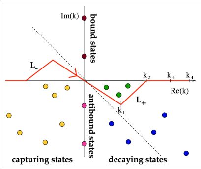
FIG. 2.: Representation of the complex $k-$plane, showing the positions of bound states, resonances, antiresonances, and the antibound states. $L_{+}$ is the contour representing the non-resonant continuum. The Berggren completeness relation involves the bound states, decaying states lying between $L_{+}$ and real $k-$axis, and the scattering states on $L_{+}$. The contour $L_{+}$ has to be chosen in such a way that all the poles in the discrete sum in Eq. (36) are contained in the domain between $L_{+}$ and the real energy axis.

Following the residuum theorem, one obtains:

$$-\int_{0}^{+\infty}|u_{k}\rangle\langle u_{k}|\,dk + \int_{L_{+}}|u_{k}\rangle\langle\widetilde{u_{k}}|\,dk$$ (26)

$$= 2i\pi\sum_{k_{n}}Res\left(|u_{k}\rangle\langle\widetilde{u_{k}}|\right)_{k=k_{n}},$$ (27)

where $k_{n}$ are the poles of $|u_{k}\rangle\langle\widetilde{u_{k}}|$ lying between the real axis and the complex contour.

In general, the scattering wave function $u_{k}$ can be written as :

$$u_{k}(r)=\sqrt{\frac{-{\mathcal{J}}^{-}(k)}{2\pi{\mathcal{J}}^{+}(k)}}u^{+}_{k}(r)+\sqrt{\frac{-{\mathcal{J}}^{+}(k)}{2\pi{\mathcal{J}}^{-}(k)}}u^{-}_{k}(r).$$ (28)

In the above expression, ${\mathcal{J}}^{\pm}$ stands for the Jost function [40]:

$${\mathcal{J}}^{\pm}(k)=u^{\pm}\frac{du}{dr}-u\frac{du}{dr}^{\pm},$$ (29)

where $u^{\pm}\sim H^{\pm}_{l,\eta}(kr)$ when $r\to+\infty$, and $u\equiv Au^{+}+Bu^{-}$. For bound and decaying states, ${\mathcal{J}}^{-}(k)$$\neq$0 (${\mathcal{J}}^{-}(k)=0$ only for capturing states with the incoming wave asymptotics). Consequently, the pole of $u_{k}(r)$ corresponds to zero of ${\mathcal{J}}^{+}(k)$. When $k\to k_{n}$, i.e., when $u_{k}$ approaches the resonant state, then:

$$|u_{k}\rangle\langle\widetilde{u_{k}}|\sim-\frac{{\mathcal{J}}^{-}(k_{n})}{2\pi{\mathcal{J}}^{+}(k)}|u^{+}_{k_{n}}\rangle\langle\widetilde{u^{+}_{k_{n}}}|.$$ (30)

The derivative of the Jost function at $k=k_{n}$ is

$$\left[\frac{d{\mathcal{J}}}{dk}\right]_{k=k_{n}}=i{\mathcal{J}}^{-}(k_{n})Reg\left[\int_{0}^{+\infty}\!\!\!\!{u^{+}_{k_{n}}}^{2}(r)\,dr\right].$$ (31)

As this derivative is nonzero, we have as $k\to k_{n}$:

$${\mathcal{J}}^{+}(k)\sim(k-k_{n})\left[\frac{d{\mathcal{J}}^{+}}{dk}\right]_{k=k_{n}},$$ (32)

hence

$$|u_{k}\rangle\langle\widetilde{u_{k}}|\sim-\frac{1}{2\pi i(k-k_{n})}|u_{n}\rangle\langle\widetilde{u_{n}}|,$$ (33)

where the normalized resonant state is:

$$u_{n}(r)=u^{+}_{k_{n}}(r)\left(Reg\left[\int_{0}^{+\infty}\!\!\!\!{u^{+}_{k_{n}}}^{2}(r)\,dr\right]\right)^{-\frac{1}{2}}.$$ (34)

Finally, the residuum at $k=k_{n}$ is

$$Res\left(|u_{k}\rangle\langle\widetilde{u_{k}}|\right)_{k=k_{n}}=-\frac{1}{2i\pi}|u_{n}\rangle\langle\widetilde{u_{n}}|$$ (35)

and the completeness relation follows immediately:

$$\sum_{n}|u_{n}\rangle\langle\widetilde{u_{n}}|+\int_{L_{+}}|u_{k}\rangle\langle\widetilde{u_{k}}|\,dk=1.$$ (36)

In the above equation $|u_{n}\rangle$ are the Gamow states (both bound states and the decaying resonant states between the real $k-$axis and the complex contour). Relation (36) is the Berggren completeness relation which allows one to expand the states with complex $k$ inside the zone between real $k-$axis and the complex contour. One may notice again that the resonances in Eq. (34) are normalized using the squared wave function and not the modulus of the squared wave function. This is a consequence of the analytical continuation which is used to introduce the normalization of Gamow states.

Figure 2 illustrates the ingredients entering Eq. (36). The resonant states, the poles of the $S$ matrix, are represented by the dots. They are divided into the bound, decaying, capturing, and antibound states (see, e.g., Refs. [34, 41, 38]). The relation (36) involves the bound and decaying states and the contour $L_{+}$ lying in the fourth quadrant of the complex-$k$ plane.

In practical applications, one has to discretize the integral in (36) [42, 43]:

$$\int_{L_{+}}|u_{k}\rangle\langle\widetilde{u_{k}}|\,dk\simeq\sum_{i=1}^{N_{d}}|u_{i}\rangle\langle\widetilde{u_{i}}|,$$ (37)

where $u_{i}(r)=\sqrt{\Delta_{k_{i}}}u_{k_{i}}(r)$ and $\Delta_{k_{i}}$ is the discretization step. It follows from the definition of $u_{i}(r)$ that

$$\langle u_{i}|\widetilde{u_{j}}\rangle=\delta_{i,j},$$ (38)

and the discretized Berggren relation (36) takes the form:

$$\sum_{n}|u_{n}\rangle\langle\widetilde{u_{n}}|+\sum_{i=1}^{N_{d}}|u_{i}\rangle\langle\widetilde{u_{i}}|\simeq 1.$$ (39)

This relation is formally identical to the standard completeness relation in a discrete basis and, in the same way, leads to the eigenvalue problem $H|\Psi\rangle=E|\Psi\rangle$. However, as the formalism of Gamow states is non-hermitian, the matrix $H$ is complex symmetric.

Up to this point, the choice of the contour in Eq. (2) has been completely arbitrary. In practice, however, one wants to minimize the number of discretization points $N_{d}$ along $L_{+}$. This can be achieved if the scattering functions on the contour (or, rather, their phase shifts) change smoothly from point to point. This condition can be met if the contour does not lie in the vicinity of a pole, especially the narrow resonant state. If this condition is met, the states appearing in the basis (39) can be naturally divided into:

• Bound states – lying on the imaginary $k$-axis (or negative real energy axis),

• Narrow decaying states – lying close to and below the real $k$-axis (or below the positive real energy axis). Those states can be interpreted as physical resonances of the system,

• Non-resonant continuum – represented by the scattering states along $L_{+}$. Physically, those are the building blocks of the non-resonant background.

These definitions can be extended to many-body states in the complex energy (or momentum) plane. In the following, we shall clearly distinguish between resonant, resonance, and non-resonant states.

The completeness relations derived above hold in every $(j,\ell)$ channel. Consequently, in practical calculations, one has to take different contours for different partial waves. As discussed below, the choice of the contour depends on the distribution of resonant states in the complex $k$-plane.

In a number of papers (see, e.g., Refs. [44, 45, 46]), resonant states were applied to problems involving continuum in the so-called pole expansion, neglecting the contour integral in Eq. (36). The importance of the contour contribution was investigated in Refs. [47, 48, 25, 26, 27] where it was concluded that if one is aiming at a detailed description, the non-resonant contribution must be accounted for. This point will be clearly seen in several examples discussed below.

A Completeness of the one-body Berggren basis: illustrative examples

In this section, we shall discuss examples of the Berggren completeness relation in the one-body case. The s.p. basis is generated by the spherical Woods-Saxon (WS) potential:

$$V(r) = -V_{0}f(r)-V_{\rm so}4\vec{l}\cdot\vec{s}\frac{1}{r}\frac{df(r)}{dr},$$ (41)

$$f(r) = \left[1+\exp\left({\frac{r-R_{0}}{d}}\right)\right]^{-1}.$$ (42)

In all examples of this section, the WS potential has the radius $R_{0}$ = 5.3 fm, diffuseness $d=0.65$ fm, and the spin-orbit strength $V_{so}$ = 5.0 MeV. The depth of the central part is varied to simulate different situations.

The complex contour corresponds to three straight segments in the complex $k-$plane, joining the points: $k_{0}=0.0-i0.0$, $k_{1}=0.2-i0.2$, $k_{2}=0.5-i0.0$ and $k_{3}=2.0-i0.0$. The contour is discretized with a different number of points: $n$=60, 80, 100, 120, 160, and final results are obtained using the Richardson extrapolation method. In the examples considered in this section, we shall expand the $2p_{3/2}$ state, $|u_{\rm WS}\rangle$, either weakly bound or resonant, in the basis $|u_{\rm WS^{B}}(k)\rangle$ generated by the WS potential of a different depth:

$$|u_{\rm WS}\rangle = \sum_{i}c_{k_{i}}|u_{\rm WS^{B}}(k_{i})\rangle$$ (43)

$$+ \int_{L_{+}}c(k)|u_{\rm WS^{B}}(k)\rangle\,dk,$$ (44)

cf. Eq. (36). In the above equation, the first term in the expansion represents contributions from the resonant states while the second term is the non-resonant continuum contribution. Since the basis is properly normalized, the expansion amplitudes meet the condition:

$$\sum_{i}c^{2}_{k_{i}}+\int_{L_{+}}c^{2}(k)\,dk=1.$$ (45)

In all cases considered, the $0p_{3/2}$ and $1p_{3/2}$ orbitals are well bound (by $\sim 40$ MeV and $\sim 18$ MeV, respectively) and do not play any role in the expansion studied.

In the first example, we shall expand the $2p_{3/2}$ s.p. resonance (0.25–i0.20 MeV) of a WS potential of the depth $V_{0}$=58 MeV in the basis generated by the WS potential of the depth $V_{0}^{B}$=59 MeV (here the $2p_{3/2}$ s.p. resonance has an energy of 0.16–i0.09 MeV). The density of the expansion amplitudes is shown in Fig. 3. One can see that the contribution from the non-resonant continuum is essential even though the $2p_{3/2}$ basis state is a resonance. In this example, as one might expect, the contribution from the resonance state in the basis is dominant.

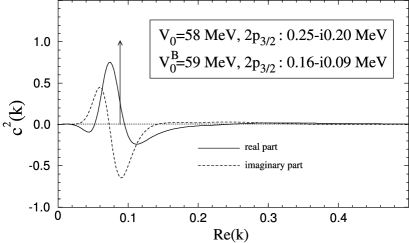
FIG. 3.: Distribution of the squared amplitudes $c^{2}(k)$ of the s.p. state $2p_{3/2}$ of one WS potential ($V_{0}$ = 59 MeV) in the s.p. basis generated by another WS potential ($V_{0}^{(B)}$=58 MeV). The amplitudes of both real (solid line) and imaginary (dashed line) parts of the wave function are plotted as a function of Re[$k$]. The height of the arrow gives the squared amplitude of the $2p_{3/2}$ resonance contained in the basis.

The second example shown in Fig. 4 deals with the case of a $2p_{3/2}$ state that is bound in both potentials. Here $V_{0}$=64 MeV and $V_{0}^{(B)}$=62 MeV, and the $2p_{3/2}$ state lies at $-$0.91 MeV and $-$0.33 MeV, respectively.

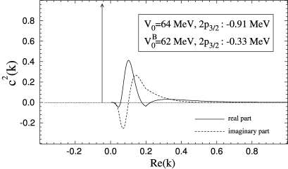
FIG. 4.: Similar as in Fig. 3 but for the bound $2p_{3/2}$ s.p. state of the WS potential with $V_{0}$=64 MeV expended in the basis generated by another WS potential ($V_{0}^{(B)}$ = 62 MeV). The height of the arrow gives the squared amplitude of the bound $2p_{3/2}$ state at the value of -Im[$k$] (the corresponding $k-$value is purely imaginary).

As in the previous case, the contribution from the resonant (here: bound) state in the Berggren basis dominates and the contribution of the non-resonant continuum is small although non-negligible. In this figure, one can notice the small cusp at Re[$k$]=0.2, even though the density $c^{2}(k)$ is an analytic function of $k$. This apparent paradox is due to the fact that $c^{2}(k)$ is plotted as a function of Re[$k$] (Im[$k$]=0). Moreover, the path in the complex plane is continuous but not derivable at $k$ = $0.2-i0.2$. These two aspects contribute to the appearance of the ‘discontinuous feature’, which of course has no physical meaning.

An interesting situation is presented in Fig. 5. Here the unbound $2p_{3/2}$ state ($V_{0}$=59 MeV) is expanded in a WS basis containing the bound $2p_{3/2}$ level ($V_{0}^{(B)}$=62 MeV). Consequently, the non-resonant continuum has to supply the imaginary part of the resonance’s wave function.

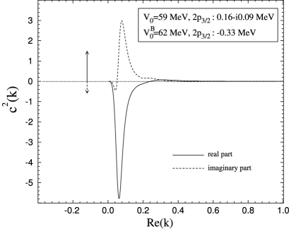
FIG. 5.: Similar as in Fig. 3 except for the $2p_{3/2}$ resonance of the WS potential with $V_{0}$=59 MeV expended in the basis generated by another WS potential ($V_{0}^{(B)}$ = 62 MeV).

The last example (Fig. 6) corresponds to $V_{0}$=64 MeV and $V_{0}^{(B)}$=59 MeV. This is the most intriguing case since one expresses a bound (real) state in the basis which contains only complex wave functions (the contribution from well bound $0p_{3/2}$ and $1p_{3/2}$ s.p. states is negligible). In this case, the non-resonant continuum annihilates the imaginary component of the $2p_{3/2}$ s.p. resonance contained in the basis. Indeed, in this example, the contribution from the contour is dominant.

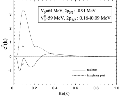
FIG. 6.: Similar as in Fig. 3 except for the $2p_{3/2}$ bound state of the WS potential with $V_{0}$=64 MeV expended in the basis generated by another WS potential ($V_{0}^{(B)}$=59 MeV) containing a resonance.

To see the convergence of the wave function obtained by the expansion method, in Fig. 7 we show the root mean square (RMS) deviation of the calculated $2p_{3/2}$ wave function from the exact result as a function of the number of discretization points along the contour. While the wave functions converge fairly quickly, the convergence of complex energies is slightly slower; hence, one has to employ the Richardson extrapolation method to get an energy precision of the order of a keV.

FIG. 7.: The root mean square (RMS) deviation of the $2p_{3/2}$ wave function of the WS potential ($V_{0}=64$ MeV) obtained by a diagonalization in a basis generated by another WS potential ($V_{0}^{B}$=59 MeV) from the exact wave function (obtained by a direct integration of the Schrödinger equation). The RMS deviation is shown as a function of the number of discretization points along the $2p_{3/2}$ contour.

IV Gamow Shell Model Hamiltonian

The GSM Hamiltonian applied in this work consists of a one-body term and a zero-range two-body interaction. The spherical one-body potential was taken in a WS form (41). In our study, resonant states are determined using the generalized shooting method for bound states which requires an exterior complex scaling. The numerical algorithm for finding Gamow states for any finite-depth potential has been tested on the example of the Pőschl-Teller-Ginocchio (PTG) potential [49], for which the resonance energies and wave functions are known analytically. Energies of all PTG resonances with a width of up to $90$ MeV are reproduced with a precision of at least $10^{-6}$ MeV.

Contrary to the traditional shell model, the effective interaction of CSM cannot be represented as a single matrix calculated for all nuclei in a given region. The GSM Hamiltonian contains a real effective two-body force expressed in terms of space, spin, and isospin coordinates. The matrix elements involving continuum states are strongly system-dependent, and they have to be determined for each case separately. This creates an additional difficulty, but there is also a pay-off. Namely, the resulting two-body matrix elements fully take into account the spatial extension of s.p. wave functions.

In this work, as a residual interaction we took the surface delta interaction [50]

$$V(1,2)=-V_{\rm SDI}\delta\left(\vec{r}_{1}-\vec{r}_{2}\right)\delta(r_{1}-R)$$ (46)

with the the same value of $R$ as in the WS potential. In our exploratory GSM calculations, we consider two cases: (i) the chain of oxygen isotopes with the inert ¹⁶O core and active neutrons in the $sd$ shell, and (ii) the helium chain with the inert ⁴He core and active neutrons in the $p$ shell. The parameters of the GSM Hamiltonian are summarized in Table I. The WS potentials have been adjusted to s.p. states in one-neutron nuclei ¹⁷O and ⁵He. For ¹⁷O, the resulting WS $0d_{5/2}$ and $1s_{1/2}$ states are bound, with s.p. energies -4.142 MeV and -3.272 MeV, respectively, and $0d_{3/2}$ is a resonance with the s.p. energy 0.898–i0.485 MeV. The agreement with experimental data ($e_{5/2_{1}^{+}}^{exp}$=–4.143 MeV, $e_{1/2_{1}^{+}}^{exp}$ = -3.273 MeV, and $e_{3/2_{1}^{+}}^{exp}$ = 0.942 MeV, $\gamma_{3/2_{1}^{+}}^{exp}$ = 96 keV) is excellent. The strength of the SDI has been adjusted for a given configuration space to the experimental two-neutron separation energy of ¹⁸O. Since only $0d_{3/2}$ is a s.p. resonance, we shall include only a $d_{3/2}$ non-resonant continuum. In fact, the completeness relation requires taking the non-resonant continua corresponding to all partial waves ($\ell,j$). However, if for a given partial wave no resonances are included in the basis, the corresponding non-resonant continua can be chosen along the real momentum axis. Since, to the first order, the inclusion of these continua should only result in the renormalization of the effective interaction, they can be ignored in most cases, except for Sec. V B.

Variant	$R(fm)$	$d(fm)$	$V_{0}(MeV)$	$V_{\rm so}(MeV)$	$V_{\rm SDI}$
	$(fm)$	$(fm)$	$(MeV)$	$(MeV)$	$(MeV\,fm^{3})$
17O	$3.05$	$0.65$	$55.8$	$6.06$	$700$
5He	$2.00$	$0.65$	$47.0$	$7.50$	$1670$

TABLE I.: Parameters of the GSM Hamiltonian used in the calculations for the oxygen isotopes (“¹⁷O” parameter set) and the helium isotopes (“⁵He” parameter set): WS radius $R$, WS diffuseness $d$, WS strength $V_{0}$, spin-orbit strength $V_{\rm so}$, and strength of the residual SDI interaction $V_{\rm SDI}$.

The nucleus ⁵He, with one neutron in the $p$ shell, is unstable with respect to the neutron emission. Indeed, the $J^{\pi}=3/2_{1}^{-}$ ground state of ⁵He lies 890 keV above the neutron emission threshold and its neutron width is large, $\Gamma$=600 keV. The first excited state, $1/2_{1}^{-}$, is a very broad resonance ($\Gamma$=4 MeV) that lies 4.89 MeV above the threshold. Our WS potential yields single-neutron resonances $p_{3/2}$ and $p_{1/2}$ at $E$=0.745–i0.32 MeV and $E$=2.130–i2.936 MeV, respectively. In our model space we take resonances $0p_{3/2}$, $0p_{1/2}$, and the two associated complex continua $p_{3/2}$ and $p_{1/2}$. The strength of the SDI has been adjusted for a given configuration space to the experimental two-neutron separation energy of ⁶He.

For the $N$-body problem, the Hamiltonian matrix contains one- and two-body matrix elements. The one-body part corresponds to s.p. energies of basis states and contributes only to diagonal matrix elements. In general, the calculation of two-body matrix elements is performed by splitting the radial integral into 16 terms corresponding to all different possible asymptotic conditions of s.p. wave functions. Then, each term is regularized separately by an appropriate choice of angle of the external complex scaling, cf. Sec. II.

V Many-body completeness relation with Gamow states

The discretized basis (39) can be a starting point for establishing the completeness relation in the many-body case, in a full analogy with the standard shell-model in a complete discrete basis, e.g., the harmonic oscillator basis. In this case one has:

$$\sum_{n}|\Psi_{n}\rangle\langle\widetilde{\Psi_{n}}|\simeq 1,$$ (47)

where the $N$-body Slater determinants $|\Psi_{n}\rangle$ have the form $|\phi_{1}\ldots\phi_{N}\rangle$, where $|\phi_{k}\rangle$ are resonance (bound and decaying) and scattering (contour) s.p. states. The approximate equality in (47) is an obvious consequence of the continuum discretization, similarly as in (39). Like in the case of s.p. Gamow states, the normalization of the Gamow vectors in the configuration space is given by the squares of shell-model amplitudes:

$$\sum_{n}c_{n}^{2}=1,$$ (48)

and not to the squares of their absolute values.

In the particular case of two-particle states, the completeness relation reads:

$$\sum_{i_{1},i_{2}}|\phi_{i_{1}}\;\phi_{i_{2}}\rangle_{J}\,{{}_{J}}\langle\phi_{i_{1}}\;\phi_{i_{2}}|\simeq 1.$$ (49)

This relation can be used to calculate the two-body matrix elements.

A Determination of many-body bound and resonance states

Before discussing completeness relations in the many-body case, let us describe the method of selecting many-body resonances. In a standard shell model, one often uses the Lanczos method to find the low-energy eigenstates (bound states) in very large configuration spaces. This popular method is unfortunately useless for the determination of many-body resonances because of a huge number (continuum) of surrounding many-body scattering states, many of them having lower energy than the resonances. A practical solution to this problem is the two-step procedure proposed in Ref. [25]:

• In the first step, one performs the pole approximation, i.e., the Hamiltonian is diagonalized in a smaller basis consisting of s.p. resonant states only. Here, some variant of the Lanczos method can be applied. The diagonalization yields the first-order approximation to many-body resonances $|\Psi_{i}\rangle^{(0)}$, where index $i$ ($i=1,\dots,N$) enumerates all eigenvectors in the restricted space. These eigenvectors serve as starting vectors (pivots) for the second step of the procedure.

• In the second step, one includes couplings to non-resonant continuum states in the Lanczos subspace generated by $|\Psi_{j}\rangle^{(0)}$ ($j\in[1,\dots,N]$).

• Finally, one searches among the $M$ solutions $|\Psi_{j;k}\rangle$, ($k=1,\dots,M$) for the eigenvector which has the largest overlap with $|\Psi_{j}\rangle^{(0)}$.

This procedure is a variant of the Davidson method. Obviously, in the search for bound states, both Lanczos and Davidson methods can be used. In the following, we shall show that the procedure outlined above allows for an efficient determination of physical states within the set of all eigenvectors of a given Lanczos subspace.

As a representative example, let us consider the cases of ¹⁸O and ²⁰O with the core of ¹⁶O, i.e., two- and four-particle systems, respectively. Here we employ the complex $d_{3/2}$ contour corresponding to two segments defined by the points: $k_{1}=0+i0$, $k_{2}=0.2-i0.05$, and $k_{3}=0.4-i0.0$. The contour is discretized with 17 and 9 points for ¹⁸O and ²⁰O, respectively. From all the possible many-body configurations, we only keep the Slater determinants with an energy less than 5 MeV and with a width smaller than 1.7 MeV.

The results of calculations for the $0^{+}$ states in ¹⁸O are displayed in Fig. 8.

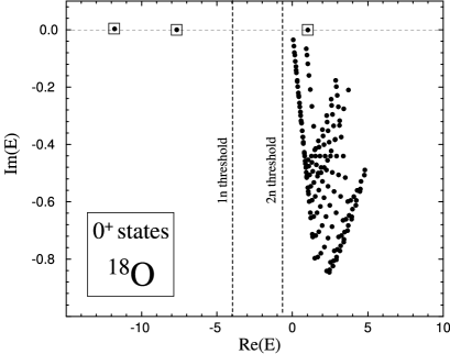
FIG. 8.: Complex energies of the $0^{+}$ states in ¹⁸O resulting from the diagonalization of the GSM Hamiltonian. One- (1n) and two-neutron (2n) emission thresholds are indicated. The physical bound and narrow resonance states are marked by squares. The remaining eigenstates represent the non-resonant continuum.

In this case, one obtains two bound states. An eigenstate lying just close to the real energy axis just above the two-neutron threshold is a candidate for a resonance. Even though the width of this state is very small, only the overlap with the states calculated in the pole approximation can give the answer. Figure  9 shows

FIG. 9.: Absolute value of the overlap between the ground state wave function $\Psi_{0}$ of ¹⁸O calculated without the coupling to the non-resonant continuum (pole approximation) and the different $0_{n}^{+}$ eigenstates $\Psi_{n}$ of the GSM Hamiltonian (calculated with the couplings to the $d_{3/2}$ non-resonant continuum), as a function of the total energy.

the overlap of the ground-state wave function $\Psi_{0}$ of ¹⁸O, calculated in the pole approximation, with all the $0^{+}$ eigenstates of the GSM Hamiltonian resulting from the full diagonalization. One can see that only one state (the GSM ground state) has a significant overlap with $\Psi_{0}$; hence, the identification of the ground state wave function is unambiguous. Figure 10

FIG. 10.: Similar to Fig. 9 except for the $0^{+}_{3}$ state wave function of ¹⁸O, $\Psi_{3}$.

illustrates a more challenging case of the third $0^{+}_{3}$ state of ¹⁸O. In spite of the fact that this state is embedded in the non-resonant $0^{+}$ continuum, its identification is straightforward. It is interesting to notice that those GSM states in Fig. 8 that represent the non-resonant background tend to align along regular trajectories. As discussed in Refs. [26, 27], the shapes of these trajectories directly reflect the geometry of the contour in the complex $k$-plane. In the two-particle case, this information can be directly used to identify the resonance states.

Figure 11 shows the results of calculations for the $0^{+}$ states in ²⁰O. As compared to the ¹⁸O case, the number of many-body states is much larger and the regular pattern of non-resonant states reflecting the structure of the contour is gone (the figure represents the projection of four-dimensional trajectories onto two dimensional space). While the two lowest (bound) states can be simply identified by inspection, for the higher-lying states it is practically impossible to separate the resonances from the non-resonant continuum. However, the procedure outlined above makes it possible to identify unambiguously the many-body resonance states. On the other hand, the method proposed in Refs. [26, 27] cannot be easily applied.

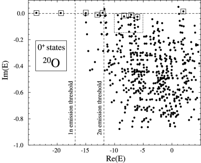
FIG. 11.: Similar to Fig. 8 except for the $0^{+}$ states in ²⁰O. The small negative widths of several unbound states are due to the fact that the number of discretization points along the contour is fairly small (5) in this case.

The many-body resonances should be stable with respect to small deformations of the contour (as the physical solutions should not be dependent on the deformation of the basis). This observation offers an independent criterion for identifying resonance states. Figure 12 shows the effect of a small deformation of the contour on the stability of selected $0^{+}$ states in ²⁰O. As expected, only the states which have previously been identified as resonances are stable with respect to small changes of the contour; the states belonging to the non-resonant continuum ‘walk’ in the complex energy plane following contour’s motion.

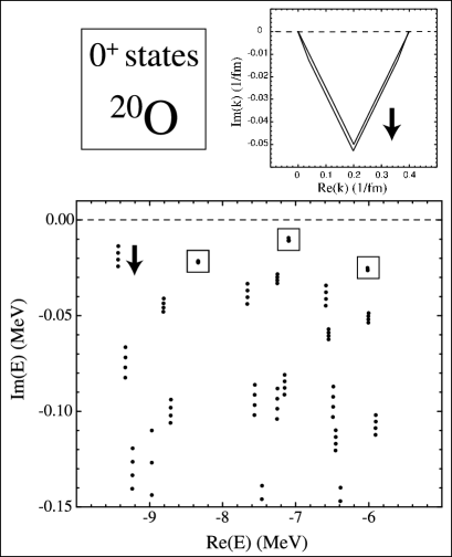
FIG. 12.: The effect of small changes in the contour on the stability of resonant and non-resonant $0^{+}$ states in ²⁰O. Top: the contour in the complex-$k$ plane corresponding to the $0d_{3/2}$ continuum. The direction of the contour’s deformation is indicated by an arrow. The calculations were performed for four contours, each divided into nine segments (i.e., 10 discretization points); only the first and maximally deformed contours are shown. Bottom: the resulting shifts in positions of many-body states corresponding to the complex energy region of Fig. 11 marked by a dotted line. It is seen that the states identified as resonant are very stable with respect to small changes of the contour, while the states representing the non-resonant continuum move significantly in the direction indicated by an arrow.

B Completeness of the many-body Gamow basis: example of two interacting particles

In this section, we shall discuss the completeness of the many-body basis spanned by Gamow states. Since the number of configurations is growing extremely fast with the number of valence nucleons, and this is enhanced by including the non-resonant continuum, we shall restrict our discussion to the case of two valence particles. By analyzing the behavior of the wave function as the number of basis states grows, one can assess the impact of various truncations in the valence space. This is especially important for calculations with zero-range forces, such as the SDI interaction employed in this work, which require an energy cut-off. In the calculations contained in this section, the configuration space consists of all the Slater determinants of energy less than 35 MeV.

As a first example, we shall consider the convergence of the ground-state energy of ¹⁸O with the increasing size of the non-resonant phase space. The GSM s.p. space consists of the $0d_{5/2}$, $1s_{1/2}$ orbitals and the $0d_{3/2}$ Gamow resonance. This discrete basis is supplemented by adding successive continua: $s_{1/2}$, $p_{1/2}$, $p_{3/2}$, …, in the decreasing order of their importance. Since $0d_{3/2}$ is a resonance, a $d_{3/2}$ contour should be complex, and we take it according to Sec. V A. Other non-resonant continua are real and for their path we choose a straight segment with $0<k<1.3$ fm^-1 . The discretization of each continuum, whether real or complex, is made with 10 points.

As one can see in Fig. 13 (top), the convergence is achieved with the $d_{3/2}$, $f_{7/2}$, $d_{5/2}$, $s_{1/2}$, and $f_{5/2}$ contours; the contributions from all the remaining partial waves with $\ell>3$ and $\ell=1$ are practically negligible.

FIG. 13.: Ground-state energy of ¹⁸O (top) and ⁶He (bottom) as a function of the number of different $(\ell,j)$ non-resonant continua in the valence space. For ¹⁸O we employ the complex $d_{3/2}-$contour consisting of three straight segments connecting the points: $k_{0}=0.0-i0.0$, $k_{1}=0.3-i0.2$, $k_{2}=0.5-i0$, and $k_{3}=1.3-i0$ (all in fm^-1).

As a rule of thumb, the continua which contribute most to the binding energy are those which are associated either with s.p. resonances in the basis or with weakly bound s.p. states. This is the case with the $0d_{5/2}$, $1s_{1/2}$, and $0d_{3/2}$ orbitals, and also with the $0f_{7/2}$ state which has an energy of +7.43 MeV and a width of 3.04 MeV. Even though this wide resonance is absent in the basis, it has nevertheless an indirect influence through the $f_{7/2}$ contour which ‘keeps memory’ of its presence. One may notice that the presence of the (complex) $d_{3/2}$ contour affects not only the real part of the ground-state energy but also its imaginary part; the ground-state energy has a spurious width of $\sim$ –130 keV in the pole approximation, and this width is reduced to $\sim$ –2 keV when the $d_{3/2}$ (10-point) contour is added. The spurious width of the ground state remains stable when other (real) contours are added.

Nucleus	Configuration	$c^{2}$
	$0d^{2}_{5/2}$	0.872+i1.146 $\times 10^{-4}$
	$1s^{2}_{1/2}$	0.044–i5.973 $\times 10^{-6}$
18O	$0d^{2}_{3/2}$	0.028–i6.624 $\times 10^{-3}$
	$L_{+}^{(1)}$	0.042+i4.709 $\times 10^{-3}$
	$L_{+}^{(2)}$	0.015+i1.795 $\times 10^{-3}$
	$0p^{2}_{3/2}$	0.891–i0.811
	$0p^{2}_{1/2}$	0.004–i0.079
6He	$L_{+}^{(1)}$	0.255+i0.861
	$L_{+}^{(2)}$	$-$0.150+i0.029

TABLE II.: Squared amplitudes of different configurations in the ground states of two-neutron systems ¹⁸O and ⁶He. The sum of squared amplitudes of all Slater determinants, including $n$ particles in the non-resonant continuum, is denoted by $L_{+}^{(n)}$. See text for details.

The structure of the ground-state wave function of ¹⁸O calculated with the full non-resonant continuum discussed in the context of Fig. 13 is given in Table II. One can see that the configuration with 2 neutrons in the $0d_{5/2}$ shell dominates; the remaining configurations, including those with one and two neutrons in the non-resonant continuum, contribute with $\sim$ 15% to the wave function. Imaginary parts of squared amplitudes are generally very small. This is due to the small width of the $0d_{3/2}$ resonance included in the basis.

As a second example, we shall investigate the energy convergence for the weakly bound ground state of ⁶He. We shall assume that the structure of ⁶He can be described in the full $0p$ shell with two valence neutrons. Since the GSM s.p. space consists of the $0p_{3/2}$, $0p_{1/2}$ Gamow resonances, the associated $p_{3/2}$ and $p_{1/2}$ non-resonant continua should be complex. Here, the $p_{3/2}$ contour consists of three straight segments connected at points: $k_{0}=0.0-i0.0$, $k_{1}=0.3-i0.35$, $k_{2}=0.5-i0$, and $k_{3}=0.7-i0$. In the $p_{1/2}$ non-resonant channel, straight lines join the points: $k_{0}=0.0-i0.0$, $k_{1}=0.4-i0.5$, $k_{2}=0.5-i0$, and $k_{3}=0.7-i0$. For all other contours we take a segment [0:0.7] fm^-1 of the real $k-$axis. The $p_{3/2}$ contour is discretized with 20 points. All other contours, including the complex $p_{1/2}-$contour, are discretized with 10 points.

As seen in Fig. 13 (bottom), the full energy convergence is attained with $p_{3/2}$ and $p_{1/2}$ contours; other scattering waves with $\ell>1$ are negligible. Coupling to the non-resonant $p_{3/2}$ and $p_{1/2}$ continua changes not only the ground-state energy but also its (spurious) width. In the pole approximation, the calculated ground state has a huge width of $\sim$ –2 MeV, which is reduced to $\sim$ –650 keV when the $p_{3/2}$ contour is added, and it reaches $\Gamma$$\sim$–10 keV when both $p_{3/2}$ and $p_{1/2}$ non-resonant continua are included. Contrary to the case of ¹⁸O, the pole approximation is totally unreliable, and it does not even give a rough approximation to the energy and wave function of the ground state of ⁶He. The main reason is that in this case one attempts to describe the bound state using the basis which does not contain any bound state and, therefore, the non-resonant continuum is essential for compensating the resonance contribution. The analogous situation, discussed in the context of a one-body problem, can be found in Sect. III A (Fig. 6).

The structure of the ground-state wave function of ⁶He including all the ($\ell,j$) continua shown in Fig. 13, is shown in Table II. One can see that the configuration with two neutrons in the $0p_{3/2}$ shell dominates, though the imaginary part of the corresponding squared amplitude is almost equal in magnitude to the real part. The amplitude of the $0p^{2}_{1/2}$ configuration is small, whereas the contributions from one and two particles in the non-resonant continuum, $L_{+}^{(1)}$ and $L_{+}^{(2)}$, are almost equally important.

VI GSM Study of oxygen isotopes

In this section we shall discuss the GSM results for a chain of oxygen isotopes with several valence neutrons ($N_{val}\geq 2$). In the calculations, we assume the core of ¹⁶O. As discussed in Sec. IV, the valence neutrons are distributed over the $1s_{1/2}$ and $0d_{5/2}$ bound shells, the $0d_{3/2}$ Gamow resonance, and the discretized $d_{3/2}$ non-resonant continuum. The complex $d_{3/2}$ contour corresponds to two segments defined by the points: $k_{1}=0+i0$, $k_{2}=0.2-i0.05$, and $k_{3}=0.4-i0.0$. It is discretized with 9 points. Consequently, the discretized s.p. GSM space (39) consists of a total of 12 subshells on which valence neutrons are distributed. Let us reiterate that we also introduce the cut-off in the configuration space of the GSM. In this study, we shall include all Slater determinants with an energy (width) smaller than 5 MeV (1.7 MeV). Moreover, we shall take only Slater determinants with, at most, 2 neutrons in the non-resonant continuum. We have checked that configurations with a larger number of neutrons in the non-resonant continuum are of minor importance in all nuclei from ¹⁸O to ²²O, and their contribution is $<$ 0.01% in all cases studied. Our aim is not to give the precise description of actual nuclei (for this, one would need a realistic Hamiltonian and a larger configuration space), but rather to illustrate the method, its basic ingredients, and underlying features.

1 Ground states of oxygen isotopes

According to our calculations (see, e.g., Table III for ¹⁸O), the ground-state wave functions of ^18-22O are dominated by the single shell model configuration $0d^{N_{\rm val}}_{5/2}$ having a weight of 80-95%; the non-resonant continuum contribution is relatively small. A one-neutron continuum provides between 0.1 and 1% of the wave function, whereas a two-neutron continuum yields a contribution which varies from $\sim 0.01$ to $\sim 0.1$% in these nuclei. This means that the main effect of the non-resonant continuum in these states is to cancel a spurious width induced by the $0d_{3/2}$ resonance included in the basis, and their influence on the real part of the energy can be neglected.

Configuration	$c^{2}$
$0d^{2}_{5/2}$	0.935+i1.836$\times 10^{-4}$
$1s^{2}_{1/2}$	0.040–i1.560$\times 10^{-5}$
$0d^{2}_{3/2}$	0.021–i4.973$\times 10^{-3}$
$L_{+}^{(1)}$	3.913$\times 10^{-3}$+i4.412$\times 10^{-3}$
$L_{+}^{(2)}$	$-$1.002$\times 10^{-4}$+i3.939$\times 10^{-4}$

TABLE III.: Same as in Table II but only including the $d_{3/2}$ contour.

It is interesting to compare the squared amplitudes for ¹⁸O in Tables II and III. The values in Table II have been obtained by taking all the contours from $s_{1/2}$ to $h_{11/2}$; whereas the results in Table III have been calculated with only a $d_{3/2}$ contour. Increasing the non-resonant space gives rise to the depletion of the occupation of bound shells.

The predicted one-neutron separation energies $S_{n}$ for oxygen isotopes are displayed in Fig. 14 and compared with the data. The calculations reproduce experimental separation energies, including the magnitude of the odd-even staggering. The difference between GSM and the data are in the worst case $\sim 500$ keV.

FIG. 14.: Calculated (crosses connected by a solid line) and experimental (circles with error bars) one-neutron separation energies in the ^18-22O chain.

2 Level schemes of oxygen isotopes

Shown in Figs. 15 - 17 are calculated and experimental spectra of ^18-20O. Let us stress that the main purpose of this comparison is to demonstrate the internal coherence of GSM results and the numerical feasibility of GSM in realistic applications. Nevertheless, in spite of the simplicity of the Hamiltonian, the overall agreement between the GSM and experimental spectra is quite reasonable.

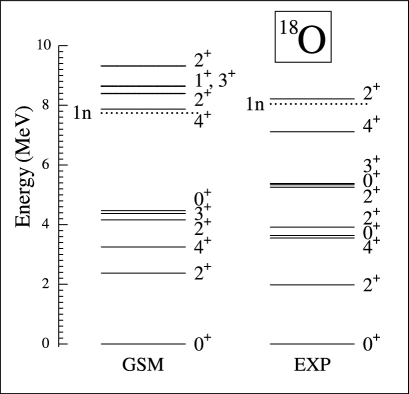
FIG. 15.: The GSM level scheme of ¹⁸O calculated in the full $sd$ space of Gamow states and employing the discretized (10 points) $d_{3/2}$ non-resonant continuum. The dashed lines indicate experimental and calculated one-neutron emission thresholds. Experimental data are taken from Ref. [51].

Figure 15 illustrates the case of ¹⁸O. One can see that the first three lowest states are relatively well described. Moreover, the one-neutron emission threshold is reproduced. In GSM, this threshold is obtained from the difference of calculated ground-state energies of ¹⁸O and ¹⁷O. It is important to note that all states above the one-neutron emission threshold are predicted to be resonances, i.e., their widths are positive, whereas all states below this threshold are calculated to have small spurious negative widths. This feature is certainly not imposed on the model and it proves both an internal consistency of the GSM as well as a correct numerical account of the completeness for many-body Gamow states. One should notice that in the calculations with a discretized continuum, it is impossible to assure that the bound states have a width exactly equal to zero. Instead, one expects that this numerical artifact of continuum discretization becomes numerically unimportant with increasing the number of points on the contour (see Table 1 of [25]). With 10-point discretization, the spurious width remains $\sim-5$ keV for all bound states of ¹⁸O, and we consider this a reasonable precision. Similarly, for resonances lying very close to the lowest particle emission threshold, hence having narrow widths, it may happen that their width results from the calculations as negative if the many-body completeness relation is numerically not well satisfied (see Fig. 11 and related discussion).

The calculated level scheme of ¹⁹O (see Fig. 16) reproduces the main experimental features. The ground state is $5/2^{+}$, as observed, but the higher-lying states $3/2^{+}_{1}$ and $1/2^{+}_{1}$ are given in the reversed order. Nevertheless, the next four states are rather well reproduced, in spite of the inversion of the $5/2^{+}_{2}$ and $3/2^{+}_{2}$ levels.

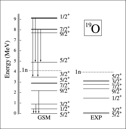
FIG. 16.: Same as in Fig. 15 except for ¹⁹O. As the number of states becomes large above the one-neutron emission threshold, only selected resonances are shown. The electromagnetic transitions listed in Table V are indicated by arrows.

Finally, the GSM prediction for ²⁰O is shown in Fig. 17. Here, the overall agreement between calculations and experiment is best for all the isotopes studied.

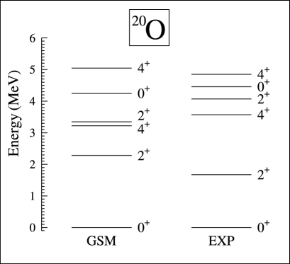
FIG. 17.: Same as in Fig. 15 except for ²⁰O.

3 Distribution of valence particles

Radial features of the density distribution of valence nucleons are always of great theoretical interest. They determine the nuclear size, electromagnetic transition rates, polarization charges, and many other nuclear properties. To assess the radial extent of the nucleonic distribution obtained in the GSM, we investigate the monopole form factor defined through the normalized radial Gamow wave functions $u_{i}(r)$ (34):

$${\rho}(r)=\sum_{i}n_{i}|u_{i}(r)\rangle\langle\tilde{u}_{i}(r)|,$$ (50)

where $n_{i}\equiv\langle a^{+}_{n}a_{n}\rangle$ is the GSM occupation coefficient of the s.p. Gamow orbital $i$. By definition, the form factor is normalized to the number of valence particles:

$$\int_{r=0}^{\infty^{\prime}}{\rho}(r)\,dr=N_{\rm val},$$ (51)

where the “prime” sign indicates that the integral is calculated by means of complex scaling.

Figure 18 shows the neutron form factors for the ground state and the highly excited resonance state $2^{+}_{5}$ of ¹⁸O.

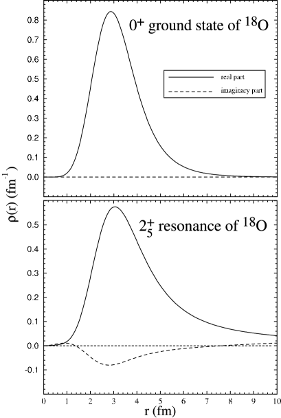
FIG. 18.: Monopole form factor of valence neutrons (50) in the ground state (top) and the $2^{+}_{5}$ resonance (bottom) of ¹⁸O. Real and imaginary parts of the density are shown with solid and dotted lines, respectively. According to definition, Eq. (51), the form factor is expressed in units of fm^-1.

As for all observables associated with bound states, the neutron form factor in the ground state of ¹⁸O is real even though the $0d_{3/2}$ resonant state is included in the basis. The imaginary part of $\rho(r)$ is very small; its value is less than $3\times 10^{-5}$ for all values of $r$. On the other hand, for the $2^{+}_{5}$ resonance, having a width of $\sim$150 keV, the form factor is always complex. This feature is not an artifact of the discretization procedure. In fact, the imaginary part of the form factor has an interesting physical interpretation. Namely, it is associated with the uncertainty in the determination of the mean value (given by the real part) [34, 52, 30, 53, 54]. In other words, in the decaying state the particle distribution cannot be given with an unlimited precision.

4 Electromagnetic transition probabilities

In the shell-model calculations with Gamow states, only radial matrix elements are treated differently as compared to the standard shell model. This means that the electromagnetic (EM) transition selection rules and the angular momentum and isospin algebra do not change. To calculate the EM transitions, one can no longer use the long wavelength approximation because of the presence of the non resonant continuum. Indeed, for the diagonal EM matrix elements $\langle n_{i}l_{i}j_{i}k_{i}|O|n_{f}l_{f}j_{f}k_{f}\rangle$ ($k_{i}$ = $k_{f}$) between the scattering states, the complex scaling cannot be carried out (see discussion around Eq. (24)). Furthermore, since in the long wavelength approximation the EM operators behave like $r^{\lambda}$, one has to deal with derivatives of delta functions, which is difficult to handle. Without the long wavelength approximation, however, these matrix elements become finite, because it is always possible to carry out a complex scaling with the Bessel function of the photon $j_{L}(qr)$, as $q\neq 0$. Moreover, as they represent a set of measure zero, the diagonal non-resonant EM matrix elements can be put to zero in the discretized calculation. As all the other matrix elements can be regularized, the EM matrix elements are all well defined.

Tables IV and V display the selected EM transition rates in ¹⁸O and ¹⁹O calculated in GSM with and without the contribution from the non-resonant $d_{3/2}$ continuum. In all calculations, we have taken the effective neutron charge $\delta e_{n}=0.5e$. While the radial form factor discussed in Sec. (VI  3) determines the structure of monopole operators, the EM probabilities probe the off-diagonal matrix elements; hence the continuum coupling manifests itself differently. As seen in Tables IV and V, the non-resonant continuum plays an important role both for transitions involving bound states only and for transitions involving an unbound state or states. In all cases, the real part of the transition rate is reasonably approximated in the pole approximation.

Similarly, as in the problem of spurious negative widths of bound states, the imaginary part of EM transitions between bound states must disappear in the limit of the non-discretized continuum. Indeed, in our calculations the imaginary part of such a transition rate tends to zero when the coupling to the non-resonant continuum is added. In the cases studied, taking only 10 points on the $d_{3/2}$ contour decreases the imaginary part by one to two orders of magnitude, depending on the transition. The real part of the transition probabilities changes by up to $\sim$ 10% when the contribution from the contour is considered. This is nevertheless an important change if one notices that the configurations with one and two neutrons in the non-resonant continuum amount to $\sim$ 0.1% of bound wave functions in these nuclei. For most transitions, the experimental values are reproduced within a factor of 3 by the GSM, and we find this agreement satisfactory in light of a very simple Hamiltonian employed.

Transition	Without contour	With contour	Exp.
$2_{1}^{+}\stackrel{{\scriptstyle\mbox{E2}}}{{\longrightarrow}}0_{1}^{+}$	2.75–i0.001	2.68–i0.011	3.32
$4_{1}^{+}\stackrel{{\scriptstyle\mbox{E2}}}{{\longrightarrow}}2_{1}^{+}$	1.99+i0.015	1.94–i0.003	1.19
$0_{2}^{+}\stackrel{{\scriptstyle\mbox{E2}}}{{\longrightarrow}}2_{1}^{+}$	1.66+i0.007	1.48+i0.006	17
$2_{2}^{+}\stackrel{{\scriptstyle\mbox{M1}}}{{\longrightarrow}}2_{1}^{+}$	0.04–i0.000	0.04–i0.000	0.14
$2_{2}^{+}\stackrel{{\scriptstyle\mbox{E2}}}{{\longrightarrow}}0_{1}^{+}$	0.19+i0.004	0.18–i0.001	1.3

TABLE IV.: Electromagnetic GSM rates (all in W.u.) for the selected transitions in ¹⁸O calculated (i) in the pole approximation without the complex-energy contour and (ii) with the $d_{3/2}$ contour representing the non-resonant continuum. Experimental data [51] are shown in the last column.

Table V displays transition rates in ¹⁹O, indicated in Fig. 16 by arrows. The three lowest transitions are between bound states and the GSM calculations with contour predict a very small imaginary part (less than 0.001 W.u.). The next four transitions in Table V involve the unbound $7/2_{2}^{+}$, $1/2_{2}^{+}$, and $5/2_{3}^{+}$ levels lying above the one-neutron threshold, and the corresponding transition rates are, in general, complex. The effect is particularly pronounced for the $1/2_{2}^{+}\stackrel{{\scriptstyle\mbox{E2}}}{{\longrightarrow}}5/2_{3}^{+}$ transition between unbound states. As mentioned in Sec. VI  3, the imaginary part gives the uncertainty of the average value [30, 53, 54]. In all cases, the real part of the matrix element is slightly influenced by the interference with the non-resonant background,

Transition	Without contour	With contour	Exp.
$3/2_{1}^{+}\stackrel{{\scriptstyle\mbox{M1}}}{{\longrightarrow}}5/2_{1}^{+}$	0.01–i0.002	0.01–i0.0	0.088
$1/2_{1}^{+}\stackrel{{\scriptstyle\mbox{M1}}}{{\longrightarrow}}3/2_{1}^{+}$	0.02–i0.003	0.02+i0.0	0.0093
$1/2_{1}^{+}\stackrel{{\scriptstyle\mbox{E2}}}{{\longrightarrow}}5/2_{1}^{+}$	3.07+i0.010	3.07+i0.003	0.58
$9/2_{1}^{+}\stackrel{{\scriptstyle\mbox{E2}}}{{\longrightarrow}}5/2_{1}^{+}$	1.78+i0.000	1.74–i0.006	$<$1
$7/2_{3}^{+}\stackrel{{\scriptstyle\mbox{E2}}}{{\longrightarrow}}5/2_{3}^{+}$	0.12–i0.062	0.13–i0.037
$1/2_{3}^{+}\stackrel{{\scriptstyle\mbox{E2}}}{{\longrightarrow}}5/2_{3}^{+}$	4.57+i0.430	4.58+i0.373
$7/2_{3}^{+}\stackrel{{\scriptstyle\mbox{E2}}}{{\longrightarrow}}3/2_{2}^{+}$	0.12+i0.038	0.13+i0.054
$1/2_{3}^{+}\stackrel{{\scriptstyle\mbox{E2}}}{{\longrightarrow}}3/2_{2}^{+}$	0.82–0.034	0.85–i0.012

TABLE V.: Same as in Table IV except for electromagnetic transitions in ¹⁹O shown in Fig. 16.

VII GSM study of helium isotopes

A description of the neutron-rich helium isotopes, including Borromean nuclei ^6,8He, is a challenge for the GSM. ⁴He is a well-bound system with the one-neutron emission threshold at 20.58 MeV. On the contrary, as discussed in Sec. IV, the nucleus ⁵He is a broad resonance. The two-neutron system ⁶He, on the contrary, is bound with the two-neutron emission threshold at 0.98 MeV and one-neutron emission threshold at 1.87 MeV. The first excited state $2_{1}^{+}$ at 1.8 MeV in ⁶He is neutron unstable with a width $\Gamma$=113 keV.

The s.p. configuration space used includes both resonances $0p_{3/2}$, $0p_{1/2}$ and the two associated complex continua $p_{3/2}$ and $p_{1/2}$, which are discretized with 5 points each. The fact that the resonances in the basis are so broad requires particular attention when selecting points along the contour. They are given in Table VI.

point No.	$p_{3/2}$	$p_{1/2}$
1	0.01$-$i0.01	0.05$-$i0.05
2	0.10$-$i0.06	0.20$-$i0.43
3	0.20$-$i0.095	0.40$-$i0.45
4	0.30$-$i0.06	0.60$-$i0.43
5	0.40$-$i0.01	0.75$-$i0.05

TABLE VI.: Discretized $p_{3/2}$ and $p_{1/2}$ contours in the complex-$k$ plane (in fm^-1) representing the non-resonant continuum in the He calculation.

In this case, we cannot significantly increase the density of points along the contour because the calculation for the heavier helium isotopes with more valence neutrons would not be feasible. On the other hand, we do not introduce any restriction on energies and widths of Slater determinants included. Also, no restriction on the number of neutrons in the non-resonant continuum is imposed, with the only exception being ⁹He, where we allow for at most 4 neutrons to occupy “contour shells”. Contrary to the discussion in Sect. V B, we neglect all remaining real continua in the present calculation. We shall see that this will have an impact on the relative weight of different configurations in the wave function.

1 Spectra of helium isotopes

The energies of the lowest GSM states of helium isotopes are shown In Fig. 19, and the structure of their ground state wave functions is given in Table VII.

Nucleus	Configuration	$c^{2}$
	$0p^{2}_{3/2}$	0.870–i0.736
	$0p^{2}_{3/2}$	0.007–i0.076
6He	$L_{+}^{(1)}$	0.271 +i0.752
	$L_{+}^{(2)}$	$-$0.147+i0.060
	$0p^{3}_{3/2}$	1.110–i0.879
	$0p^{2}_{3/2}0p_{1/2}$	0.006–i0.029
	$0p_{3/2}0p^{2}_{1/2}$	0.022–i0.042
7He	$L_{+}^{(1)}$	0.050 +i0.951
	$L_{+}^{(2)}$	$-$0.185+i0.008
	$L_{+}^{(3)}$	$-$0.002–i0.009
	$0p^{4}_{3/2}$	0.296–i1.323
	$0p^{2}_{3/2}0p^{2}_{1/2}$	$-$0.060–i0.158
	$L_{+}^{(1)}$	1.596+i1.066
8He	$L_{+}^{(2)}$	$-$0.728+i0.630
	$L_{+}^{(3)}$	$-$0.125–i0.204
	$L_{+}^{(4)}$	0.020–i0.012
	$0p^{4}_{3/2}0p_{1/2}$	0.180–i1.328
	$L_{+}^{(1)}$	1.596+i0.734
9He	$L_{+}^{(2)}$	$-$0.584+i0.801
	$L_{+}^{(3)}$	$-$0.217–i0.193
	$L_{+}^{(4)}$	0.025–i0.034

TABLE VII.: Squared amplitudes of different configurations in the ground states of ^6-9He. The s.p. space consists of both $0p_{3/2}$, $0p_{1/2}$ Gamow resonances and the two associated complex continua $p_{3/2}$ and $p_{1/2}$ which are discretized with 5 points each.

As seen in Table VII, the non-resonant continuum contributions $L_{+}^{(n)}$ are always essential, and, in some cases (e.g., ^8,9He), they dominate the structure of the ground-state wave function. Moreover, as can be seen in the example of ⁸He, configurations with many neutrons in the non-resonant continuum are essential for fulfilling the completeness relation. In this particular case, the $L_{+}^{(1)}$ contribution is even more important than the contribution from the resonant states, and even the $L_{+}^{(4)}$ configuration gives a non-negligible contribution of the order of 1-2%. ($L_{+}^{(n)}$ amplitudes seem to decrease with $n$.) Without the contour, the predicted ground-state energy of ⁸He is +2.08 MeV and the spurious width is huge, $\Gamma=-4.16$ MeV. The inclusion of scattering states lowers the binding energy to $-1.6$ MeV. Clearly, the pole approximation fails miserably in this case.

It is instructive to compare the wave function decomposition in Tables VII (only $p_{3/2}$ and $p_{1/2}$ contours are included) and II (all contours up to $f_{7/2}$ are included). As expected, the spread of the ground-state wave function over non-resonant continuum states is larger in the latter case, but this effect is relatively less important than in the case of ¹⁸O (cf. Fig. 13).

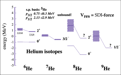
FIG. 19.: Experimental (EXP) and predicted (GSM) binding energies of ^6-9He as well as energies of $J^{\pi}$=2⁺ states in ^6,8He. The resonance widths are indicated by shading. The energies are given with respect to the core of ⁴He.

Our calculations reproduce the most important feature of ⁶He and ⁸He: the ground state is particle-bound, despite the fact that all the basis states lie in the continuum. In spite of a very crude Hamiltonian, rather limited configuration space, etc., the calculated ground state energies shown in Fig. 19 reproduce surprisingly well the experimental data. The odd-$N$ isotopes of ^7,9He are calculated to be neutron resonances. The neutron separation energy anomaly (i.e., the increase of one-neutron separation energy when going from ⁶He to ⁸He) is reproduced. One can see that ⁸He is predicted to be better bound than ⁶He, though, contrary to the data, the two-neutron separation energy of ⁸He is smaller than that of ⁶He. Also, the energies of excited $2_{1}^{+}$ states are in fair agreement with the data.

The present calculations for helium isotopes have a systematic tendency to underbind. The spurious width of the ground state of ⁸He is $\sim$ 100 keV, largely due to the $0p_{3/2}$ resonance. For that reason, the removal of the spurious width (which reflects the accuracy of our calculations) cannot be done here as precisely as in the oxygen case. In order to check the stability of the results for ^6,8He, we carried out additional calculations increasing the number of points along the complex contour. We have found that the value of the two-neutron separation energy difference, $S_{2n}(^{8}$He) - $S_{2n}(^{6}$He), which is negative with 5 states in each non-resonant continuum, depends sensitively on the number of discretization points. This is because $S_{2n}(^{8}$He) increases fast with the size of the non-resonant phase space. While with our schematic Hamiltonian we were unable to find a fully satisfactory result for the ground-state energy of ⁸He just by increasing the number of discretization points, we can see that there is a systematic improvement when the number of non-resonant shells increases. Therefore, one would be tempted to associate the so-called ‘helium anomaly’ in the position of two-neutron emission threshold when going from ⁶He to ⁸He with the strong enhancement in the occupation of non-resonant continuum states.

2 Distribution of valence neutrons in ⁶He

Form factors of valence neutrons (50) in $0^{+}_{1}$ and $2^{+}_{1}$ states of ⁶He are shown in Figs. 20.

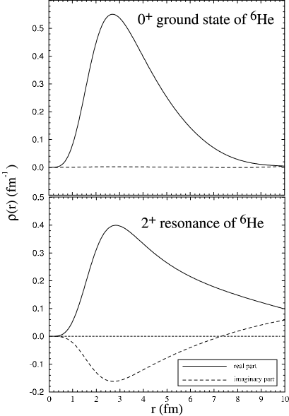
FIG. 20.: Monopole form factor of valence neutrons for the ground state (top) and for the lowest $2^{+}_{1}$ resonance (bottom).of ⁶He.

In this calculation, we have taken discretized $p_{1/2}$ and $p_{3/2}$ continua with 20 points each. Even with this very high number of continuum states, the imaginary part of the form factor in the ground state of ⁶He is still $\sim$ 2$\times 10^{-3}$ fm^-1. It is interesting to see that the radial distribution of neutrons in this case extends well above the range of the one-body potential, as expected for a weakly bound system. In the case of the first excited (resonance) $2^{+}_{1}$ state, $\rho(r)$ is complex; real and imaginary parts of the density are of a comparable size, which is obviously related to the large width ($\sim$ 500 keV) of this state.

VIII Summary

This paper contains the detailed description of the Gamow Shell Model, which can be viewed as a straightforward extension of the standard diagonalization shell model that allows for a consistent treatment of bound states and the particle continuum, including both resonances and the non-resonant background. Our first application, based on a realistic, albeit simple, two-body SDI force, concerns many-neutron systems, including states and nuclei near the neutron-emission threshold.

In this work, we succeeded in overcoming several obstacles which traditionally plagued previous continuum shell model applications. In addition to the successful inclusion of the continuum-continuum coupling by means of the complex rotation technique (exterior complex scaling), we incorporated the non-resonant part of the continuum. This has been achieved by discretizing the contour in the complex $k$-plane for each partial wave. Another problem which has been solved in our study is the isolation of resonance states. As a result of the GSM diagonalization, one obtains a multitude of states corresponding to the many-body continuum, some being resonances and some representing the non-resonant background. Our work offers a simple prescription on how to identify the resonance states from the multitude of complex-energy eigenstates of the GSM Hamiltonian.

The GSM Hamiltonian is composed of a one-body term and a two-body residual interaction which is directly written in terms of space, spin, and isospin coordinates. The two-body matrix elements have to be determined separately for each case by means of radial integration. As a result, the resulting Hamiltonian matrix fully takes into account the continuum coupling, in particular the spatial extension of s.p. wave functions, determining the physics of halo nuclei.

We demonstrated that the contribution from the non-resonant continuum is essential, especially for unbound and near-threshold states. In some cases (e.g., ^8,9He) non-resonant continuum components dominate the structure of the g.s. wave function. The so-called ‘pole approximation’ (resonant state expansion) breaks down in such cases. In addition, the inclusion of the non-resonant continuum also impacts results for bound states.

The results of our first calculations for binding energies, spectra, electromagnetic matrix elements, and nucleonic distributions are very encouraging. In particular, pairing correlations due to the continuum-continuum scattering can bind the ground states of ^6,8He with a completely unbound basis provided by the s.p. resonances of ⁵He. The ‘Helium anomaly’ (an increase in one- and two-neutron separation energy when going from ⁶He to ⁸He) is explained in terms of the neutron scattering to the non-resonant background. In all cases considered, our calculations yield neutron resonances above the calculated neutron threshold – a property that is not guaranteed a priori by the formalism.

Other applications of GSM, including the case of open proton and neutron shells, also employing more realistic effective interactions, are in progress. We are also working on the optimization of the non-resonant part of calculations (choice of the contours, distribution of discretization points, etc.). We are convinced that the Gamow Shell Model will become a very useful theoretical tool unifying structure and reaction aspects of weakly bound nuclei.

- [1] J. Dobaczewski and W. Nazarewicz, Phil. Trans. R. Soc. Lond. A 356, 2007 (1998).
- [2] E. Caurier, F. Nowacki, and A. Poves, Eur. Phys. J. A 15, 145 (2002).
- [3] E. Caurier and G.Martinez-Pinedo, Nucl. Phys. A704, 60c (2002).
- [4] T. Otsuka, Y. Utsuno, R. Fujimoto, B.A. Brown, M. Honma, and T. Mizusaki, Eur. Phys. J. A 13, 69 (2002); Eur. Phys. J. A 15, 151 (2002).
- [5] L. Coraggio, A. Covello, A. Gargano, N. Itaco, T.T.S. Kuo, D.R. Entem, and R. Machleidt, Phys. Rev. C 66, 021303 (2002).
- [6] B.A. Brown, Nucl. Phys. A704, 11c (2002).
- [7] R.G. Thomas, Phys. Rev. 81, 148 (1951); 88, 1109 (1952).
- [8] J.B. Ehrman, Phys. Rev. 81, 412 (1951).
- [9] H. Feshbach, Ann. Phys. (NY) 19, 287 (1962).
- [10] U. Fano, Phys. Rev. 124, 1866 (1961).
- [11] C. Mahaux and H. Weidenmüller, Shell Model Approaches to Nuclear Reactions (North-Holland, Amsterdam, 1969).
- [12] H.W. Bartz, I. Rotter, and J. Höhn, Nucl. Phys. A 275, 111 (1977); ibid. A 307, 285 (1977).
- [13] R.J. Philpott, Nucl. Phys. A289, 109 (1977).
- [14] D. Halderson and R.J. Philpott, Nucl. Phys. A345, 141 (1980).
- [15] I. Rotter, Rep. Prog. Phys. 54, 635 (1991), and references quoted therein.
- [16] J. Okołowicz, M. Płoszajczak, and I. Rotter, Phys. Rep. 374, 271 (2003).
- [17] K. Bennaceur, F. Nowacki, J. Okołowicz, and M. Płoszajczak, Nucl. Phys. A651, 289 (1999).
- [18] K. Bennaceur, N. Michel, F. Nowacki, J. Okołowicz, and M.Płoszajczak, Phys. Lett. 488B, 75 (2000).
- [19] K. Bennaceur, F. Nowacki, J. Okołowicz, and M. Płoszajczak, Nucl. Phys. A671, 203 (2000).
- [20] B.V. Danilin, I.J. Thompson, J.S. Vaagen, and M.V. Zhukov, Nucl. Phys. A632, 383 (1998).
- [21] E. Nielsen, D.V. Fedorov, A.S. Jensen, and E. Garrido, Phys. Rep. 347, 373 (2001).
- [22] H. Esbensen and G.F. Bertsch, Phys. Rev. C 59, 3240 (1999).
- [23] D. Eppel and A. Lindner, Nucl. Phys. A240, 437 (1975).
- [24] W.M. Wendler, Nucl. Phys. A472, 26 (1987).
- [25] N. Michel, W. Nazarewicz, M. Płoszajczak, and K. Bennaceur, Phys. Rev. Lett. 89, 042502 (2002).
- [26] R. Id Betan, R.J. Liotta, N. Sandulescu, and T. Vertse, Phys. Rev. Lett. 89, 042501 (2002).
- [27] R. Id Betan, R.J. Liotta, N. Sandulescu, and T. Vertse, Phys. Rev. C 67, 014322 (2003).
- [28] G. Gamow, Z. Phys. 51, 204 (1928); 52 510 (1928).
- [29] A.F.J. Siegert, Phys. Rev. 56, 750 (1939).
- [30] T. Berggren, Phys. Lett. B373, 1 (1996).
- [31] Y.B. Zel’dovich, JETP (Sov. Phys.) 39, 776 (1960).
- [32] N. Hokkyo, Prog. Theor. Phys. 33, 1116 (1965).
- [33] W.J. Romo, Nucl. Phys. A116, 617 (1968).
- [34] T. Berggren, Nucl. Phys. A109, 265 (1968).
- [35] B. Gyarmati, and T. Vertse, Nucl. Phys. A160, 523 (1971).
- [36] G. Garcia-Calderon and R. Peierls, Nucl. Phys. A265, 443 (1976).
- [37] V.I. Kukulin, V.M. Krasnopol’sky, J. Horác̆ek, Theory of Resonances, Kluwer Academic Publishers (Dordrecht-Boston-London), 1989.
- [38] P. Lind, Phys. Rev. C 47, 1903 (1993).
- [39] R.G. Newton, Scattering Theory of Waves and Particles (Springer-Verlag, New York Heidelberg Berlin) 1982.
- [40] R. Jost, Helv. Phys. Acta 20, 256 (1947).
- [41] T. Vertse, P. Curutchet, and R.J. Liotta, Lecture Notes in Physics 325 (Springer Verlag, Berlin 1987), p. 179.
- [42] R.J. Liotta, E. Maglione, N. Sandulescu, and T. Vertse, Phys. Lett. B367, 1 (1996).
- [43] T. Vertse, R.J. Liotta, W. Nazarewicz, N. Sandulescu, and A.T. Kruppa, Phys. Rev. C57, 3089 (1998).
- [44] G.G. Dussel, R.J. Liotta, H. Sofia, and T.Vertse, Phys. Rev. C46, 558 (1992).
- [45] S. Fortunato, A. Insolia, R.J. Liotta, and T. Vertse, Phys. Rev. C54, 3279 (1997).
- [46] O. Civitarese, R.J. Liotta, and T. Vertse, Phys. Rev. C 64, 057305 (2001).
- [47] T. Vertse, R.J. Liotta, and E. Maglione, Nucl. Phys. A584, 13 (1995).
- [48] P. Lind, R.J. Liotta, E. Maglione, and T. Vertse, Z. Phys. A347, 231 (1994).
- [49] J.N. Ginocchio, Annals of Physics (NY) 152, 203 (1984); 159, 467 (1985).
- [50] I.M. Green and S.A. Moszkowski, Phys. Rev. 139, B790 (1965).
- [51] R.B. Firestone and V.S. Shirley, Table of Isotopes, Eighth Edition, Vol. I (Wiley, New York).
- [52] B. Gyarmati, F. Krisztinkovics, and T. Vertse, Phys. Lett. 41B, 475 (1972).
- [53] C.G. Bollini, O. Civitarese, A.L. De Paoli, and M.C. Rocca, Phys. Lett. B 382, 205 (1996).
- [54] O. Civitarese, M. Gadella, and R.I. Betan, Nucl. Phys. A660, 255 (1999).