Dynamics of many-particle fragmentation in a Cellular Automaton model

Abstract

A 3D Cellular Automaton model developed by the authors to deal with the dynamics of N–body interactions has been adapted to investigate the head–on collision of two identical bound clusters of particles, and the ensuing process of fragmentation. The range of impact energies is chosen low enough, to secure that a compound bound cluster can be formed. The model is devised to simulate the laboratory set–up of fragmentation experiments as monitored by 4$\pi$ detectors. The particles interact via a Lennard–Jones potential. At low impact energies the numerical experiments following the dynamics of the individual particles indicate a phase of energy sharing among all the particles of the compound cluster. Fragments of all sizes are then found to evaporate from the latter cluster. The cluster sizes, measured in our set–up by simulated 4$\pi$ detectors, conform to a power law of exponent $\approx$ 2.6.

In an attempt to duplicate the laboratory caloric curves related in particular to nuclear fragmentation processes, we introduce several temperature parameters (kinetic temperature of nucleons, kinetic temperature of fragments, reaction equilibrium temperatures). Theoretical caloric curves are then constructed for those temperature parameters we regard as physically most relevant. Our results show that different temperature definitions generate different curve patterns, indicating that the fragmentation system remains far from thermodynamic equilibrium. The pattern of the laboratory caloric curve for Au–Au collision experiments as derived from a recent analysis [NuPECC report Dec. 1997] is reproduced qualitatively by our reaction temperatures.

I Introduction

The currently favoured theoretical approach of investigating many-particle fragmentation consists in applying statistical mechanics to the excited compound cluster. The procedure relies on the assumption that the collection of particles, or compound cluster, originating from the two colliding clusters reaches a state of thermodynamic equilibrium. The properties of this compound cluster can then be described thermodynamically, in terms of a small number of global parameters, namely the total number of particles $A$, possibly the total charge number $Z$, the total available energy $E$ (regarded as measured in the centre of mass system), the total volume $V$ occupied by the particles, and possibly the area of the surface $\Sigma$ enclosing this volume (RI01 for a recent review of the theoretical approaches in the nuclear field; CH97 ; FA97 ; GO01 ; SC01 ; SC97 ; KU99 ; BR89 for experiments and results on molecules and clusters of ions). In this Paper we shall describe a less restrictive theoretical framework applicable to a multiple fragmentation process of arbitrary nature (nuclear, atomic, or molecular). For our specific illustrations the relevant orders of magnitude of the global parameters have been chosen to capture the particular nuclear case.

A few comments on the related laboratory experiments are therefore in order. The empirical results are collected essentially through the following experimental procedure. A target nucleus ($A_{T},Z_{T}$) is bombarded with a high–energy beam of incident nuclei ($A_{I},Z_{I}$) generated by an accelerator. A series of detector set–ups (such as ALADIN, CHIMERA, EOS, FOPI, INDRA, LASSA or MINIBALL), ideally uniformly distributed over a sphere centred on the target nucleus and thereby securing a $4\pi$ coverage, identify the charge and mass of the collisional fragments as well as their kinetic energies.

Experiments of this nature were spearheaded in the 80s MI82 ; PA84 ; PA85 . In MI82 the target was a Kr or Xe ion; the accelerated incident particles consisted in a beam of protons of energy in the range 80–350 MeV. The detectors isolated nuclear fragments in the $A$–range 12 $\leq A\leq$ 31. The yield $Y(A,Z)$ was found to be consistent with an expression of the form $A^{-\tau}$ times a Boltzmann factor MI82 depending on a temperature parameter. The exponents evaluated experimentally were $\tau$ = 2.64 (Xe) and 2.65 (Kr). Qualitatively the outcome of these experiments was compared with the thermodynamic transition from a liquid phase (original target heated by the infalling beam of protons) to a state of formation of droplets of all sizes (fragment distribution measured by the detectors) taking place at a critical–point temperature $T_{c}$. In fact, for the latter transition a power–law in the sizes of the droplets is known to hold, of exponent $\tau$ = 2.33. This result is derived in the context of the mean field theory JA83 . Similar fragmentation experiments were described in PA84 ,PA85 , in which the target was an Ag, Kr, Xe or U ion; the incident particles were protons or carbon ions. Again fragments were detected (here in the $Z$–range 3 $\leq Z\leq$ 22), which obeyed an approximate power law.

The seemingly canonical interpretation of these earlier as well as of the more recent intermediate–mass ion–ion collision experiments (for instance the ¹⁹⁷Au–¹⁹⁷Au fragmentation reported on in PO95 ,NU97 ) regards the fragmentation process as the formal analogue of a liquid–gas phase transition occurring at a transition temperature $T_{c}$. At lower temperatures, $T<T_{c}$, the nuclear system is a mixture of individual nucleons and fragments (liquid phase); at higher temperatures, $T>T_{c}$, all fragments dissolve into a gas of nucleons (gas phase).

This interpretation of an observed fragmentation process (of any nature) as a thermodynamic phase transition may be helpful in providing a qualitative picture for the outcome of the collision experiments. However, it should be clear that a many–body fragmentation process induced by violent collision cannot be regarded as a proper thermodynamic equilibrium phenomenon. Prior to the collision, both the target cluster, and the incident cluster, are in a stable internal equilibrium state. The two clusters are characterised globally by two sets of (extensive) thermodynamic variables $(A_{q},Z_{q},E_{q},V_{q},{\Sigma}_{q})$, $q$ = $T,I$. The energies $E_{q}$ are measured in the centre–of–mass (CM) system of ions $T$ and $I$ respectively. The stability of the equilibrium of each cluster requires a zero surface pressure. At the moment of the incipient collision the $T$ and $I$ clusters merge into a single cluster $C$, the compound cluster $C$ (counterpart of the compound nucleus $C$ in the sense of Bohr and Wheeler BO39 ). The extensive thermodynamic variables are then essentially the sums of the extensive variables of the components $T$ and $I$, $A_{C}=A_{T}+A_{I}$, etc, except for the difference in the evaluation of the energy. The energy of $C$, $E_{C}$, is to be measured in the CM frame of the compound system, so that we have $E_{C}=E_{T}+E_{I}+E_{imp}$; the extra energy component, $E_{imp}$, is the impact energy (global kinetic energy of the $T$ and $I$ in CM of $C$).

Since the impact energy is a free parameter, the surface pressure of $C$, the initial merger of $T$ and $I$, will not vanish in general, and hence the compound cluster will not be in a state of thermal equilibrium. The surplus energy is expected to create a pressure increase (positive surface pressure), which will force $C$ globally to expand. This expansion may consist in a release of clusters of particles which ultimately become independent fragments (as observed in the experiments), leading in turn to a contraction of a central core. Such a phenomenon of global expansion made up of an expanding outer envelope (together with a contracting inner core) is familiar in gravitationally bound systems (spherical clusters of stars; cf the classic analysis by Lynden–Bell and Wood LY68 ). In the general fragmentation problem, the central remainder $C^{\prime}$ is a new compound cluster, with fewer particles, which keeps evaporating fragments, thereby transforming again into a smaller central cluster $C^{\prime\prime}$, as long as it has not reached a final equilibrium state. These comments make it manifest that a priori the distribution of fragments as measured by the laboratory detectors is not directly related to a statistical equilibrium state of a central cluster $C$; it is rather the system’s non–equilibrium state that causes the evaporation of the fragments. However, provided that the central cluster evolves slowly enough, the component particles may have time to reach an approximate statistical equilibrium. The latter alternative is envisaged in gravitational systems as well. The distribution of the clusters that evaporate at a given time $t$ is then expected to correspond to a chemical reaction equilibrium, or a dissociation equilibrium, at the temperature characterising the central cluster at time $t$. On the other hand, it is clear that this situation can hold only if the impact energy remains low enough. At higher impact energies the target will be essentially transparent to the particles of the incident cluster.

The simplest statistical models by–pass the conceptual question of whether or not a statistical equilibrium holds in the fragmentation process. In these models the system of particles is enclosed in an energetically insulated box of finite volume $V_{B}$; the collection of interacting particles is then fully specified by 3 independent thermodynamic parameters, $V_{B}$, $A_{C}$, and $E_{C}$ (total energy) which are given at the outset. Such a system is necessarily due to relax eventually towards a thermodynamic equilibrium. In the specific nuclear context, detailed classical molecular dynamics (CMD) calculations have indeed demonstrated directly the existence of a statistical equilibrium state, from which the thermodynamic properties of the system can be recovered AI88 , FI86 . Moreover, the distribution of the fragments with size can be evaluated in the thermal equilibrium state. Similar thermodynamic equilibrium results have also been derived in the framework of cellular automaton (CA) numerical experiments (in 2D AL99 and 3D AL00 ). However, the connection between these, as well as other theoretical models so far proposed RI01 on the one hand, and the real, a priori far from equilibrium laboratory experiments on the other hand, remains entirely unclear.

In this Paper we pursue the goal of setting up a theoretical framework capable of closely simulating the arrangement of the actual laboratory experiments. To this end (1) we follow in the first place the dynamics of the collision (as in the case of CMD calculations) without relying on an assumption of a thermodynamic equilibrium. (2) Next we analyse the collection of fragments which have arrived at a certain distance $d_{D}$ from the collision site where they can be regarded as independent. The fragment distribution is estimated at that particular level. Our procedure of evaluation of the theoretical distribution thus contrasts with the conventional statistical methods which have been applied by previous authors, including ourselves FI86 ; AL99 ; AL00 . It conforms instead essentially to the laboratory readings as given by an array of detectors located at a distance $d_{D}$ from the collision site. (3) We introduce and compute explicitly a variety of formal temperature parameters, namely kinetic temperatures associated with the gas of particles and the gas of fragments, and reaction temperatures related to the distribution of the fragments. If the system were in a state of genuine thermodynamic equilibrium, in particular during the initial stage of the collision when the two colliding clusters merge into a single compound cluster, then a true thermodynamic temperature would exist. Under this condition the formal temperature parameters would all be equal to the true temperature. Provided only that there are experimental procedures replicating the conditions of the theoretical definitions of these formal temperature parameters, the latter continue to provide a useful global characterisation of the system, whether or not a thermodynamic equilibrium state is realised: An acceptable theory must then be capable of duplicating the experimentally available values of these formal parameters.

The question of the temperatures is analysed in greater detail in Section 5. The dynamical calculations (Section 4) are carried out in the context of the Cellular Automaton (CA) model developed by the authors and discussed in AL99 and its 3D extension AL00 . A major difference between the numerical experiments of AL00 and the experiments of the present work resides in the fact that the system of component particles was confined to a finite box, while in principle the system of particles in our present analysis evolves in a virtually infinite lattice space.

The detailed CA experiments we report on refer to a nuclear fragmentation involving collisions between identical ions (cf the ¹⁹⁷Au–¹⁹⁷Au collision of ALADIN, PO95 ). We treat these collisions as being head–on. In a future work we plan to extend our model to deal with collisions of non–zero impact parameter.

II The CA Model

The CA framework adapted to the simulation of the classical dynamics of interacting particles is discussed in AL99 , for the specialised nuclear context; the particles are nucleons, and we consider low enough energies. We indicate here only the particular features of this model when applied to the collisional dynamics we are concerned with, and recall the typical orders of magnitude of the model parameters.

II.1 Geometry of Lattice Space. Particle Kinematics

Our CA universe $U$ is a cubic lattice of $L^{3}$ cells, of toroidal topology (periodic boundaries), with a typical size $L$ = 127. A lattice cell is identified by a position vector ${\bf r}$ of integer Cartesian coordinates ${\bf r}$ = $(x,y,z)$, with $x,y,z$ taking the values $-(L-1)/2$, $-(L-1)/2+1$, $\ldots$, -1, 0, 1, $\ldots$, $(L-1)/2-1$, $(L-1)/2$. An individual cubic cell has a side ${\lambda}$ chosen of the order of magnitude of the range of the nuclear forces ($\approx$ 2 fm). The timestep ${\Delta\tau}$ is of the order of the collision time of nucleons in a bound nucleus ($\approx$ 10^-23 s). Time intervals are measured by an integer $t$ (number of timesteps counted from the beginning of the experiment).

The real nucleon is simulated by a particle of mass $m$; this particle is either at rest (symbolized by the zero vector ${\bf e}_{0}$); or in a state of motion with a single absolute value of the velocity

$$v\ \ =\ \ \frac{\lambda}{\Delta\tau}.$$ (1)

Accordingly, in our framework the allowed states of motion of a particle are v = $\pm v{\bf e}_{i}$, where ${\bf e}_{i}$ represents the unit vector along the lattice axis $i$ = $x,y,z$. A CA particle $\alpha$ then exists in one among 7 possible dynamic states ${\bf v}_{\alpha}$ = 0, $v{\bf e}_{x}$, $-v{\bf e}_{x}$, $v{\bf e}_{y}$, $-v{\bf e}_{y}$, or $v{\bf e}_{z}$, $-v{\bf e}_{z}$; the momentum of this particle is denoted by ${\bf p}_{\alpha}$ (= $m{\bf v}_{\alpha}$). As in AL99 we do not take account of the charge of the nucleons.

Our CA particles obey an exclusion principle, in the sense that a cell is not allowed to contain more than one particle in the same state of motion. Accordingly, the maximum density of our nuclear matter is 7 particles per cell.

II.2 Particle Interactions and Dynamics

To simulate the interactions of a given nucleon $\alpha$ with the rest of the nucleons of our system we choose an ‘interaction neighbourhood’ of cell ${\bf r}$ containing nucleon $\alpha$, $N_{\rm int}({\bf r})$. This neighbourhood is the collection of cells made up of the central cell ${\bf r}$, the $\varphi$=6 cells which have common faces ($\phi$), the $\epsilon$=12 cells which have common edges (e), and the $\nu$=8 cells which have common vertices (v) with the ‘central’ cell ${\bf r}$. Nucleon $\alpha$ in cell ${\bf r}$ interacts with any nucleon in a cell ${\bf r^{\prime}}$ if and only if $\bf r^{\prime}$ $\in$ $N_{\rm int}({\bf r})$.

The pair interaction energy between a particle in cell $\bf r$ and a particle in cell $\bf r^{\prime}$, $V_{\rm pair}({\bf r},{\bf r^{\prime}})$, is represented by a step potential: $V_{\rm pair}({\bf r},{\bf r^{\prime}})$ = $V_{\phi}$ if both cells have a common face; $V_{\rm pair}({\bf r},{\bf r^{\prime}})$ = $V_{e}$, and $V_{\rm pair}({\bf r},{\bf r^{\prime}})$ = $V_{v}$, if they have a common edge, or a common vertex respectively. For a pair of particles in the same cell r we adopt a potential of the form $V_{\rm pair}({\bf r},{\bf r};p)$ = $V_{o}$ + $(p-1)\Delta V$; the pair–parameter $p$ takes account of the effect that the interaction energy between a pair of particles in the same cell depends on the number of different pairs present in the cell: If there are 3 particles, and hence 3 pairs, the first pair has an energy $V_{o}$, the second pair an energy $V_{o}+\Delta V$, and the third pair an energy $V_{o}+2\Delta V$. The total potential in cell r is then the sum of the pair potentials due to all particles in the interaction neighbourhood $N_{\rm int}({\bf r})$.

In order to minimize the number of free parameters of our model we have set $V_{\phi}$ $\equiv$ $V_{o}$ (equal to the interaction energy of a single pair in a cell), and $V_{e}$ $\equiv$ $V_{v}$ $\equiv$ $V_{1}$. We are then left with 3 independent energy parameters specifying the pair–interaction potential. The orders of magnitude adopted for the latter are $V_{o}$ = -3.0 MeV and $V_{1}$=-0.3 MeV; $\Delta V$ = +1.0 MeV. The precise values are adjusted to obtain optimal agreement with the observations, in particular to secure the experimental mean binding energy per nucleon, of -8 MeV in an intermediate–mass nucleus. The value of $\Delta V$ has been estimated by requiring that 2 and 3 particles in a cell form a stable bound configuration; a larger number of particles per cell leads to an unstable configuration.

Due to the discrete nature of the allowed CA states of motion, a particle suffers a change of momentum which obeys Newton’s law of motion in a statistical sense only. Two or more particles in a same cell undergo a scattering which satisfies linear momentum conservation. The computational details of the treatment of the transitions among the particle states of motion are given in AL99 .

II.3 Fragmentation Clusters and Cluster Configurations

A major aim of our simulation consists in constructing the distribution law of the fragmentation clusters as actually registered by real laboratory detectors, in the form of the number of fragments, $N$, against size, $a$ (and at fixed time $t$), $N$ = $N(a,t)$. In our experiments the ‘size’ of a cluster is understood as the number of particles in the cluster. The particles are indiscernible, so that any permutation among them which does not alter the occupation of the individual cells, does not produce a new cluster.

A fragmentation cluster of size $a$ of our CA context is eventually identified with a fragment of the laboratory nuclear fragmentation process. It simulates a nucleus containing $a$ = $A$ nucleons. The experimental counterpart of our theoretical distribution, $N(a,t)$, which ignores the charge of the fragments, is then the distribution of the isobars as resulting from the laboratory fragmentation process.

The precise specification of what we understand by a ‘cluster’ of size $a$ that takes due account of the interactions included in our model is given in the Appendix. For the purposes of computing reaction temperatures, we need to evaluate the number of distinct configurations (‘multiplicities’) of the different cluster–geometries compatible with a cluster of specified size. This question is also dealt with in the Appendix.

III The Set–up of the Numerical Experiments

All of our experiments are carried out in the CM reference frame whose origin coincides with cell $(0,0,0)$.

III.1 Initial Configuration

The initial conditions for a dynamic run are as follows. We simulate two nuclei, referred to as the ‘incident nucleus’ $I$ and the ‘target’ $T$, by two identical clusters (in the sense of our definition) located in the half–lattice $x<0$ and $x>0$ respectively. The centres of mass of the clusters $I$ and $T$ are required to lie on the $x$–axis. The mirror–symmetry demands that we have ${\bf r}_{I}$ = $(-x_{M},0,0)$ and ${\bf r}_{T}$ = $(+x_{M},0,0)$ respectively. The number of particles (and mass, in units of the nucleon mass $m$) of each cluster is $A_{T}$ = $A_{I}$ = $A$ = 150.

Initially we assign each cluster cell a single particle, so that the initial volumes of the clusters are $V$ = $A$ ${\lambda}^{3}$. The shapes of these clusters are chosen to approximate densely packed spheres. This geometry leads to a radius–mass relation of the standard type

$$R\ \ =\ \ \left(\frac{3}{4\pi}\right)^{1/3}\ \ \lambda\ \ A^{1/3}.$$ (2)

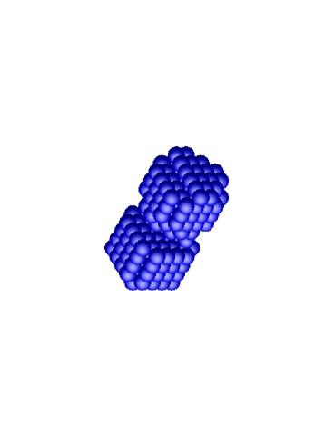
Figure 1: Initial spatial configuration ($t$=0) for head–on collision of two identical nuclei, $T$, $I$, of mass 150. Direction of propagation: $x$–axis. $T$ and $I$ separated by empty layer of cells $x$ = 0.

Overall consistency with the empirical $R$–$A$ relation then requires $\lambda$ $\approx$ 1.9 fm. The value we have adopted for our model is $\lambda$ = 1.95 fm, which produces the matter density of a real nucleus of mass $A=150$. At time $t=0$ the two clusters are just in contact (Fig. 1).

III.2 Initial Motion

Dynamically, all particles of each initial cluster, $I$ and $T$, are in ordered motion. In the CM frame of $T+I$, any particle of the target cluster has a velocity ${\bf v}_{T}$ = $-v{\bf e}_{x}$, while the velocity of any particle in the incident cluster is ${\bf v}_{I}$ = $-{\bf v}_{T}$ = $+v{\bf e}_{x}$. The ordered microscopic motion accounts for the initial macroscopic motion of the two clusters along the $x$–axis. The linear momentum of the global system $T+I$ is zero in this frame. The available impact energy is

$$E_{imp}\ \ =\ \ 2\ \ A\ K\ ,\ \ \ K\ =\ \frac{1}{2}m\ v^{2}.$$ (3)

This energy is transformed into excitation energy of the compound cluster; it leads eventually to the break–up of the latter. (As in the traditional statistical models, we ignore here particle–creation processes, in particular pion formation). The actual collision occurs at timestep $t=1$. Prior to the collision the model describes two clusters $T$ and $I$ in uniform motion in the CM frame, with opposite linear momenta ${\bf p}_{T}$ = $-A$ $mv$ ${\bf e}_{x}$ and ${\bf p}_{I}$ = $+A$ $mv$ ${\bf e}_{x}$ = $-{\bf p}_{T}$. The velocities of the two clusters are opposite, of absolute value

$$|{\bf v}_{T}|\ \ =\ \ |{\bf v}_{I}|\ \ =\ \ v.$$ (4)

III.3 The Cluster Detectors

In the laboratory experiments the detectors, which identify and count the fragments, and measure their kinetic energies, are ideally distributed isotropically around the collision centre. We achieve an acceptable approximation to isotropy respecting the lattice symmetry of our CA environment by placing our theoretical counting devices on the 6 faces (CA lattice planes) of a cube of size $2d_{D}+1$ centred at the origin of the lattice (limiting planes defined by $x$ = $\pm d_{D}$; $y$ = $\pm d_{D}$; $z$ = $\pm d_{D}$). In conformity with the laboratory experiments, the distance $d_{D}$ must be chosen macroscopically large. The minimum requirement is that $d_{D}$ exceeds the distance $d_{int}$ over which the fragments interact (freeze–out radius). For our typical cell size $\lambda$ and for initial clusters of 150 nuclei each moving along the $x$–axis test runs indicate that $d_{int,x}$ $\approx$ $d_{int,y}$ $\approx$ $d_{int,z}$ $\approx$ 20. In our numerical experiments we have chosen $d_{D}$ as large as computationally possible ($d_{D}$ $\approx$ 50 for our CA universe of size $L$=127).

IV Fragment Identification and Counting Algorithm

In models of statistical equilibrium, in which the fragments are confined to a fixed finite volume $V_{B}$, the cluster identification and count can be carried out with a standard algorithm that consists in scanning the whole box available to the fragments ST97 . However, in the real laboratory experiment the detectors are not uniformly distributed over a volume, so that the standard algorithm does not duplicate the experimental procedure. The fragment counting method we have set up in our simulation is devised to reproduce the principle of the laboratory counting procedure.

We isolate the ‘new’ clusters, $\Delta N(a;t;x^{+})$, which ‘pierce’ face $x=+d_{D}$ (our $x^{+}$ counter) of the cube at timestep $t$. The total number of clusters of size $a$, $N(a;t;x^{+})$, which have been traced by counter $x^{+}$ up to step $t$, is then the sum of all ‘new’ clusters identified from timestep 1 up to timestep $t$. We have

$$\begin{split}N(a;t;x^{+})\ \ &=\ \ \Delta N(a;t;x^{+})\ \ +\ \ N(a;t-1;x^{+})\\ &=\ \Delta N(a;t;x^{+})\ +\ \Delta N(a;t-1;x^{+})\ +\ldots+\Delta N(a;1;x^{+})\ .\end{split}$$ (5)

The identification at the other counters $x^{-}$, (face $x=-d_{D}$); $y^{+}$, $y^{-}$, (faces $y=\pm d_{D}$); $z^{+}$, $z^{-}$, (faces $z=\pm d_{D}$), follows the same scheme. The total number of all distinct clusters $N(a;t)$ traced up to time $t$ is the sum over the measurements of all 6 detectors.

The relative distribution of the fragments, $Pr(a)$, probability of a fragment of size $a$, is given by

$$Pr(a)\ =\ \lim_{t\to\infty}\ \frac{N(a;t)}{N(t)},\ \text{with}\ N(t)\ \equiv\ {\sum_{a=1}^{2A}N(a;t)}.$$ (6)

Finally, if we repeat the same simulation a large number $r$ of times, we have

$$\langle Pr(a)\rangle\ =\ \frac{\sum_{c=1}^{r}{N}^{(c)}(a;t)}{\sum_{c=1}^{r}{N}^{(c)}(t)}\ =\ \frac{\sum_{c=1}^{r}{N}^{(c)}(t){Pr}^{(c)}(a)}{\sum_{c=1}^{r}{N}^{(c)}(t)}.$$

where ${N}^{(c)}(t)$ is the total number of fragments of all sizes, ${N}^{(c)}(a;t)$ is the fragment distribution, and ${Pr}^{(c)}(a)$ is the relative fragment distribution in the $c^{th}$ experiment. If the number $r$ of experiments is chosen large enough, a stable and well defined distribution is expected to emerge.

To find $\langle Pr(a)\rangle$ we have developed a straighforward algorithm for the identification of fragmentation clusters of size $a$ which enter the plane $x=+d_{D}$ at step $t$. The algorithm exploits the property that since a free fragment propagates with speed $v$, $\Delta N$ represents the number of fragmentation clusters which intersect the plane $x=+d_{D}$, but which do not intersect the plane $x=+d_{D}+1$.

To the extent that our CA model incorporates an acceptable approximation to the physics of the fragmentation process, the relative fragment distribution as derived from our simulations should duplicate the laboratory distribution ${Pr}^{(lab)}(a)$ as measured by real detectors. In fact, consider a laboratory run of total duration $t_{exp}$, operating under stationary conditions. We then have a constant flux of infalling particles colliding with a flux of target particles. Under typical operating conditions these collision processes are binary collisions (each individual collision process occurs independently of the other collision processes). Collision $c$ therefore produces in the array of detectors a distribution given by Eq. (6). If $r(t_{exp})$ is the total number of collisions which occur over the whole run of the experiment, then the detectors register the following relative fragment distribution

$${Pr}^{(lab)}(a)\ =\ \frac{\sum_{c=1}^{r(t_{exp})}{N}^{(c)}(a;t)}{\sum_{c=1}^{r(t_{exp})}{N}^{(c)}(t)}\ =\ \frac{\sum_{c=1}^{r(t_{exp})}{N}^{(c)}(t){Pr}^{(lab,c)}(a)}{\sum_{c=1}^{r(t_{exp})}{N}^{(c)}(t)}.$$

The notations adopted in these expressions are essentially the same as in the theoretical case (${N}^{(c)}(a;t)$, ${N}^{(c)}(t)$: fragment numbers in collision $c$; ${Pr}^{(lab,c)}(a)$: relative fragment distribution of the $c^{th}$ collision; ${Pr}^{(lab)}(a)$: final average relative experimental distribution of the fragments).

V Dynamic Results

The evolution of the particles of the two colliding clusters is followed with our CA program over a total time–interval $t_{max}$ not exceeding $(L-1)-(d_{int}+d_{D})$ (about 70 in our experiments). The order of this time interval is fixed by the observation that it is the shortest time it takes an individual particle, or a cluster, ejected in the collision, to migrate through the available CA lattice, to be reflected on the boundary of the lattice universe, and to be sent back to a detector plane. For times $t>t_{max}$ a reflected fragment could collide with outflowing fragments; this would violate our assumption of non–interaction of the fragments at distances exceeding $d_{int}$.

We begin with a discussion of a first physically realistic effect.

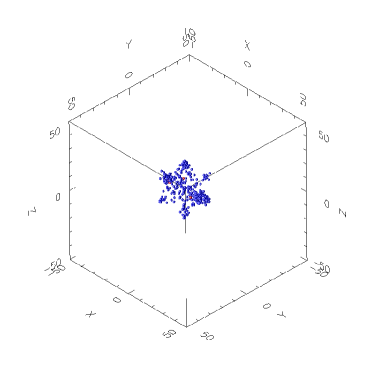
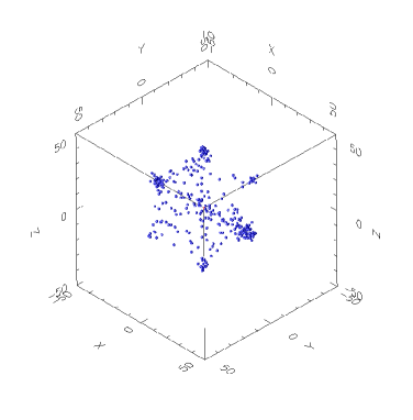
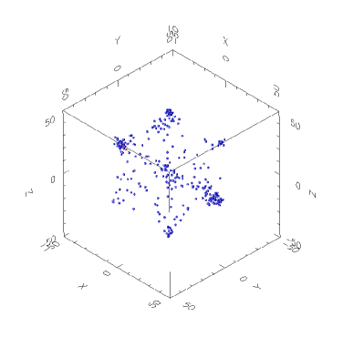
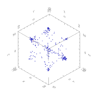
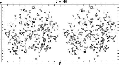
Figure 2: Configuration of fragments at timesteps $t$ = 20 (panel a), 40 (b), 50 (c), and 60 (d). Reconstructed symmetrized distribution of nucleons for timestep 40 (b^′).

(i) At the collision site we observe a central concentration of nucleons (a compound nucleus) of size $A_{C}(t)$. This concentration progressively loses individual particles as well as fragments. The sequence of frames (a), (b), (c), (d) exhibited in Fig. 2 and corresponding to an impact energy per nucleon $E_{imp}/A$ = 3.75 MeV, illustrates this situation in greater detail. Frame (a) ($t$ = 20) indicates that besides isolated particles leaving the centre two large fragments were symmetrically ejected along the collision line; smaller fragments were blown along the $y$– and $z$–axes normal to the collision line ($x$–axis). The collision site remains a high density zone, which is clearly visible on the later frames (b), (c), (d) ($t$ = 40, 50, and 60). An evaporation of small fragments and individual particles continues from this central condensation zone, at a rate which is expected to depend on the impact energy, $E_{imp}$ (the only free parameter of our series of experiments).

The experiment seems to suggest that the collision phenomenon is actually a two–stage process. In the first phase of the collision, the nucleus is broken up into several large fragments; the latter are the larger the higher the impact energy is; for a high enough impact energy, only 2 fragments emerge from the collision (negligible interaction between the two nuclei). The second phase, starting at some timestep $t_{o}$, is a more gentle evaporation from a central fragment.

To quantify the phenomenon of emission of clusters we fix a small reference volume (a cube of 21³ cells) which encloses the compound nucleus, and which we regard as a rough approximation to the space occupied by the latter. It is then reasonable to assume that the rate of particle loss from this reference volume is proportional to some a priori unknown power $\delta$ of an excess number of particles over an equilibrium number, $A_{o}$, in the reference volume, or

$$d/dt\ A_{C}\ =\ -\ \beta(E_{imp})\ (A_{C}-A_{o})^{\delta}\ ,\ \ \beta(E_{imp})\ =\ \gamma\ {E_{imp}}^{1/2}.$$ (7)

The functional form of $\beta(E_{imp})$ follows from a dimensional scaling argument. In our series of experiments in which the impact energy alone is regarded as a parameter, all other free coefficients being held fixed, we can express mass in terms of the nucleon mass, and volume in the reference volume, so that mass and volume (and hence length) become dimensionless; in this system the impact energy has the dimension of an inverse time squared. Hence the above relationship. The remaining factor $\gamma$ depends on the model constants (i.e., reference volume, mass of nucleons, nuclear interaction constants, etc).

Integration of Eq. (7), from the moment $t_{o}$, at which evaporation starts, to the current time $t$, yields

$$(A_{C}(t)-A_{o})^{1-\delta}\ =\ (A_{C}(t_{o})-A_{o})^{{1-\delta}}\ -\ (1-\delta)\ (t-t_{o})\ {E_{imp}}^{1/2}\ \gamma,\ \ {\rm if}\ \ \delta\neq 1,$$

$${A_{C}(t)\ -\ A_{o}}\ =\ (A_{C}(t_{o})-A_{o})\ \exp[-{E_{imp}}^{1/2}\ \gamma\ (t-t_{o})],\ \ {\rm if}\ \ \delta=1.$$

Fig. 3 shows the curves $(A_{C}(t)-A_{o})^{k}/(A_{C}(t_{o})-A_{o})^{k}$ for values of $k$ (=1- $\delta$) ranging from 0.1 to 0.5 (fine lines), as well as $\ln[A_{C}(t)-A_{o}]/\ln[A_{C}(t)-A_{o}]$ (heavy line); time is measured with $t_{o}$ taken as origin. The parameters $t_{o}$ and $A_{o}$ are read off from the numerical run ($t_{o}$ = 11; $A_{o}$ = 36 in the case of the experiment exhibited in Fig. 3). The curves in Fig. 3, which are strongly nonlinear for larger values of $k$, tend to become linear in the limit $k\to$ 0, as is found from a linear regression analysis (over the 25 timesteps shown). Hence Eq. (7.b) ($\delta$ = 1) gives the best fit. In other words, the excited compound cluster essentially suffers a standard disintegration. The decay time for the specific experiment we have displayed is $\tau_{dis}$ = 6.58.

(ii) A second conspicuous feature of the plot of our numerical results is an artefact of the CA lattice symmetry and computational procedure. In each lattice direction, $\pm{\bf e}_{i}$, $i=x,y,z,$ we observe a column of particles or clusters that propagate all with maximum speed $v$ (Eq. 1) away from the collision site.

Fig. 2 discloses that the density of particles in each column increases with distance, with a peak density at the two ends of each column. The peak density corresponds to the effect of the violent break–up occurring in the first phase of the collision. The subsequent gentle decrease in time of the content of the residual compound cluster, $A_{C}(t)$, implies that the rate of evaporation (Eq. 7) decreases with time as well. Therefore the density in the columns decreases as we approach the central compound cluster; at the latter central cluster, the common centre of the columns, a density maximum survives.

Statistically the particle distribution at any time $t$ preserves the symmetry of the initial configuration. Fig. 2 demonstrates indeed that the pattern possesses the following symmetry elements: The $x$– axis is a fourfold axis; the planes $(x,y)$ and $(x,z)$, as well as their bisectors are reflection planes; the $y$ and $z$–axes are binary axes, and so are the two diagonal axes; $(y,z)$ is a reflection plane. The invariance group of this statistical configuration is $D_{4h}$ (in standard notations for the point–groups; cf Landau–Lifshits, Quantum Mechanics). The distribution of the particles along the collision axis $x$ is clearly seen to be different from the distributions along the $y$ or $z$–axes, (cf in particular the large fragments on the $x$ axis). The collision axis remains a privileged direction all over the experiment.

At timestep $t$ = 0, the initial conditions of the collision set–up in our CA lattice environment, Fig. 1, create a symmetry breaking from the original octahedral (plus translational) symmetry of the empty (infinite) lattice (the ‘vacuum state’), $O_{h}$, to the symmetry $D_{4h}$ of our initial configuration. At all later times, $t>0$, our CA results demonstrate that the latter symmetry is statistically preserved (cf Fig. 2). The collision process itself, starting at $t$ = 1, induces no overall geometric symmetry transition. The occurrence of such a transition would be direct evidence for a second order phase transition. If a second order phase transition does occur in the fragmentation process, then it must be related to a finer symmetry breaking not immediately manifest in the spatial distribution of the fragments.

The initial conditions for a head–on collision of two identical nuclei occurring in the continuous physical configuration space break the symmetry of the original ‘vacuum’ (spherical plus translational symmetry) transforming it into a cylindrical symmetry, of axis coinciding with the collision axis, $K_{h}\to D_{\infty h}$. Provided that our discrete CA model can capture the essential physics of the real fragmentation mechanism, the results of the above numerical experiments are indicative that the full cylindrical symmetry should be preserved in the real laboratory experiment. This symmetry is indeed consistent with the $4\pi$ detector measurements.

Our next task is an attempt at wiping out the CA artefact (ii) in the computed spatial distribution and to convert the latter into a form more directly comparable with the laboratory experiments.

We reconstruct a $D_{\infty h}$–symmetric number distribution, $\rho^{rec}({\bf r};t)$, from the CA $D_{4h}$–symmetric number distribution, $\rho^{CA}({\bf r},t)$, by the following procedure. We expand the new distribution in Legendre polynomials

$$\rho^{rec}({\bf r};t)\ =\ \sum_{n=0}^{\infty}\ \rho_{n}(r;t)\ P_{n}(\cos\theta),$$ (8)

where the angle $\theta$ is the angle between the position vector ${\bf r}$ and the collision axis (oriented from the $I$ to the $T$ nucleus). Since the CA experiments indicate that the difference in the distribution along the collision axis and the axes normal to the collision axis is relatively small, we truncate the expansion after the dipole terms. In this lowest order approximation we then write

$$\rho^{rec}({\bf r};t)\ =\ \rho_{c}(r;t)\ +\ \eta(r;t)\ \cos\theta.$$

The functions $\rho_{c}(r;t)$ and $\eta(r;t)$ are then determined from the CA distribution by

$$\rho_{c}(r;t)\ =\ B\ \langle\rho^{CA}({\bf r};t)\rangle_{y,z},$$

$$\rho_{c}(r;t)\ +\ \eta(r;t)\ =\ B\ \langle\rho^{CA}(0,r,0;t)\rangle_{x},$$

where the righthand sides are averages over the positions $r$ = $|y|$ and $|z|$ on the $y$ and $z$ axes, and $r$ = $|x|$ on the $x$ axis respectively; $B$ is a normalisation constant which is fixed by requiring that the integration of the distribution over the available space (the sum of $\rho^{rec}({\bf r};t)$ over all CA cells ${\bf r}$) is equal to the total number of nucleons (=300 in our experiments).

Panel (b^′) of Fig. 2 shows a stereoscopic plot of the symmetrized space distribution (8) reconstructed from the CA distribution displayed in panel (b). The plot is generated by a straightforward Monte–Carlo procedure distributing 300 particles in conformity with the statistical law (8.a). We observe that this distribution falls off with distance $r$ from the centre (with an exponent $<2$), except that the higher density of the distribution front survives. We should point out that the method just redistributes the individual particles without conserving the clusters.

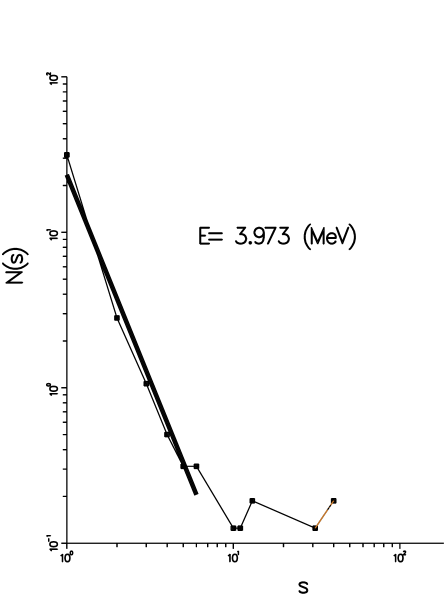
Figure 4: Cluster distribution $\log$ $N$ – $\log$ $a$ derived from simulated $4\pi$ detectors, (a) $E_{imp}/A$ = 0.307 MeV per nucleon: $\tau$ = 2.56; (b) $E_{imp}/A$ = 3.973 MeV per nucleon: $\tau$ = 2.64. The numbers of clusters are normalized to the numbers of runs.

(iii) The cluster–size distribution as generated by our CA dynamics and registered by our counters $x^{+}$,etc, obeys a power law. This result is illustrated in greater detail in Fig. 4 , which exhibits two instances, one at very low impact energy, $E_{imp}/A$ = 0.307 MeV (panel a), and the other at a 13 times higher energy $E_{imp}/A$ =3.973 MeV (panel b). The plot shows (a non–normalised form of) relation (6) in log–log format, obtained from a total number of runs $r$ = 16. Over the range $a$ $<$ 10, both curves appear as straight lines, with negative slopes $\tau$ = 2.56 (low energy) and 2.64 (high energy). Our experiments indicate that this property holds at least up to $E_{imp}/A$ $\approx$ 10 MeV, where $\tau$ takes the value 2.65. We are entitled to conclude that in the range of impact energies $E_{imp}/A$ $<$ 10 MeV, the (smaller) fragments obey a power law with negative slope $\tau$ $\approx$ 2.6, which is independent of the energy. As the impact energy increases larger clusters are being formed; the tail of the distribution then tends to become longer.

Critical exponents $\tau$ of 2.64 and 2.65 have been measured in the laboratory, for the fragment distribution of proton–Kr and proton–Xe fragmentation. We should mention also that in the field of ion cluster fragmentation, fragment distributions obeying power laws of exponents of 2.56 and 2.63 FA97 have been isolated.

It appears that the slope values of the fragment distribution we obtain from our dynamic results are in better agreement with the laboratory data than the values derived from standard statistical theories, which are close to the value given by mean field theory (JA83 : $\tau$ = 2.33). This remains also true for ion cluster fragmentation problems, even though our model parameters were not adjusted to that particular situation.

VI Formal Temperatures. Comparison with Laboratory Experiments

With the exception of the symmetrised distribution (8), the results described in the previous Section are direct results of our $N$–body simulations. They involve no extra approximations besides the assumptions inherent in any CA modellisation (space and time discretisation) and the schematisation of the interaction potential among particles. In particular, the dynamic calculations dispense with the hypothesis of formation of a compound cluster in the collision process. Our numerical experiments indicate that a configuration showing a higher central concentration, which we refer to as the compound cluster, always emerges in the simulation (Fig. 2), provided only that the collision energy is low enough as compared to the binding energy of the nucleons in the nuclei. The compound cluster (i.e. high central concentration) survives over a period of time which can be estimated from Eqs. (7).

Within this compound cluster, and, in principle, also within our CA universe $U$ (127³ cells; toroidal topology), a variety of statistical equilibria $e$, $e^{\prime}$, $e^{\prime\prime}$, $\ldots$ are conceivable among the different components.

(a) If we identify the components as the individual particles (nucleons in our specific nuclear fragmentation simulation; etc) of a configuration $Z$, then we may have a statistical equilibrium in $Z$, ${e_{E}}^{n(Z)}$, due to energy exchange ($E$) among the particles ($n(Z)$) of configuration $Z$. The configuration $Z$ may be the compound cluster $C$, or our entire CA universe $U$.

(b) If we identify the components as the clusters of particles $c$ (which in turn, when evaporating from the compound cluster become the observable fragments), then we may have (i) a statistical equilibrium due to energy exchange among the clusters of a configuration $Z$, $c(Z)$, ${e_{E}}^{c(Z)}$. But we may also have (ii) an equilibrium due to exchange of energy as well as particles ($P$) among these clusters, ${e_{E,P}}^{c(Z)}$. Under the latter alternative, the observed distribution of fragments against size will be the thermal reaction–equilibrium distribution of the clusters. For the sake of completeness we mention further (iii) that within each individual cluster $c_{f}$, the component particles may exchange energy among each other; this process may then lead to a special type of equilibrium, ${e_{E}}^{n(c_{f})}$, inside each cluster $c_{f}$.

We define here a temperature parameter $T(e)$, which is associated with a specific thermodynamic equilibrium process $e$, as follows : The parameter $T(e)$ is the thermodynamic temperature that reproduces the macroscopic properties of the specific equilibrium $e$ assuming it is realized. If $\omega$ = $F(e;T)$ is the thermodynamic relation that expresses the observable $\omega$ as a function of the thermodynamic temperature $T$ under equilibrium conditions $e$ (other thermodynamic variables being held fixed), then from the measurement of $\omega$ and the thermodynamic relation we set $T(e)$ $\equiv$ $T$. (Note that our way of introducing temperatures differs from the more formal procedure adopted in Chernomeretz et al. CH01 ). We are free to use this thermodynamic relation in a formal way to determine a parameter $T(e)$ characterising a given macroscopic configuration, whether or not the specific equilibrium $e$ holds. We begin with listing the thermodynamic relations of relevance for our purposes.

In principle, all of the above–listed equilibria, $e$, $e^{\prime}$, $e^{\prime\prime}$, $\ldots$ may arise in our numerical experiments, or in the laboratory experiments (in the sense that there is for instance no membrane surrounding a fragment that would prevent the exchange of particles, etc). The question is rather: Given an equilibrium process $e$, does the collision system we investigate survive over a time–span that is long enough for the equilibrium $e$ to establish itself?

If the collision system reaches a full thermodynamic equilibrium, then we must have

$$T(e)\ =\ T(e^{\prime})\ =\ \ldots\ \equiv\ T\ ,$$ (9)

where the formal temperatures $T(e)$, $\ldots$ obtained as indicated; all of these formal parameters are then equal; they define the single thermodynamic temperature $T$. Conversely, if relation (9) is violated, then the relevant statistical equilibria are not realized. We have indeed good reasons to believe that some of the possible equilibria listed above will never materialize in our system (cf below); or, alternatively, some equilibria cannot establish themselves over certain ranges of the impact energy. Our numerical results confirm this point.

Even if a state of full thermal equilibrium is not attained for the system we are investigating, the formal temperatures, $T(e)$, $T(e^{\prime})$, $\ldots$, may remain perfectly useful parameters for the purposes of comparison of the numerical results with actual laboratory experiments in the following sense. Suppose a given observable $\Omega$, measured in the laboratory, is plotted against the temperature parameter, $T(e)$, $\Omega$ = $Q(T(e))$, this temperature being measured according to a well–defined protocol (cf above). A typical instance is provided by the (formal) caloric curve, $T({e_{E,P}}^{c(C)})$ vs $E_{imp}$, (equilibrium process: energy and particle exchange among clusters in the compound cluster). The necessary condition for a given theoretical model, such as our present CA model, to be an adequate model for the fragmentation process, is then that this model can duplicate the experimental $\Omega$ = $Q(T(e))$ relation. The agreement must hold provided that the formal parameter $T(e)$ be obtained in conformity with the experimental protocol. It should be kept in mind that there is no guarantee that an easily measurable temperature parameter of our CA gas (such as $T({e_{E}}^{n(U)})$ can be substituted to the actual experimental parameter (temperature associated with ratio of yields $T({e_{E,P}}^{c(C)})$ ).

We have measured the following collection of temperature parameters for our CA system (adapted to nuclear fragmentation).

VI.1 Nucleon-gas temperatures: Global nucleon–gas temperature, $T_{n(U)}(t)$, and nucleon–gas temperature in compound nucleus, $T_{n(C)}(t)$

The temperature parameters $T_{n(U)}(t)$ and $T_{n(C)}(t)$ are the formal temperatures of a gas of nucleons in thermal equilibrium under exchange of energy in the CA universe $U$ and in the compound nucleus $C$ respectively. With the above notations $T_{n(U)}(t)$ $\equiv$ $T({e_{E}}^{n(U)};t)$, $T_{n(C)}(t)$ $\equiv$ $T({e_{E}}^{n(C)};t)$; the extra argument $t$ indicates that these parameters depend on time.

The total number of nucleons of our system, the CA universe $U$, is conserved, $A_{U}(t)$ $\equiv$ $A$ (=300). The number of nucleons in the compound nucleus $C$ at timestep $t$, $A_{C}(t)$, is variable, and so are the number of nucleons in motion in the universe, $A_{m(U)}(t)$, and the number of nucleons in motion in the compound nucleus, $A_{m(C)}(t)$. The temperature parameters, which are measures of the average kinetic energy per nucleon of the gas of nucleons in $U$ and $C$ respectively, are then given in terms of these numbers of nucleons by the following expressions

$$\frac{3}{2}\ \ k\ T_{n(U)}(t)\ =\ \frac{1}{2\ A}\ m\ \sum_{\alpha=1}^{A}({\bf v}_{\alpha}(t))^{2}\ =\ \frac{A_{m(U)}(t)}{A}\ K\ \ <\ \ K,$$ (10)

$$\frac{3}{2}\ \ k\ T_{n(C)}(t)\ =\ \frac{1}{2\ A_{C}(t)}\ m\ \sum_{\alpha=1}^{A_{C}(t)}({\bf v}_{\alpha}(t))^{2}\ =\ \frac{A_{m(C)}(t)}{A_{C}(t)}\ K\ \ <\ \ K.$$ (11)

In these expressions $k$ is the Boltzmann constant, ${\bf v}_{\alpha}(t)$ is the velocity of the nucleon labelled ${\alpha}$ and taken at timestep $t$, and $K$ is the kinetic energy of a moving CA particle (Eq. 3). Note that all formal temperature parameters we shall introduce are time–dependent.

The second temperature parameter, $T_{n(C)}$ (Eq. 11), measures the physically meaningful average kinetic energy of a gas of particles in the compound cluster, which can in principle reach a thermal equilibrium in our CA model, or in the laboratory; hence it can represent a genuine temperature of a gas of nucleons. This is the case if the energy exchanges among the nucleons have time to establish themselves, i.e., if the lifetime of the central condensation (cf Eqs. 7) exceeds the average collision time among nucleons in $C$ (a few timesteps).

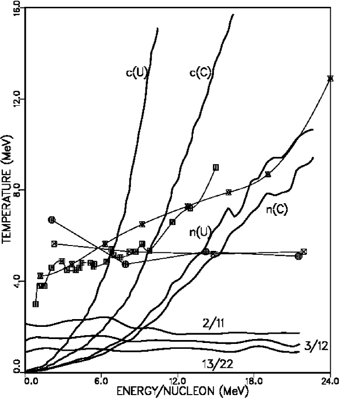
Figure 5: Formal CA caloric curves, $T$–$E_{imp}/A$, for different definitions of temperature: (a) $T_{n(C)}$, nucleon–gas in compound nucleus; ($a^{\prime}$) $T_{n(U)}$, nucleon–gas in CA universe; (b) $T_{c(C)}$, cluster–gas in compound nucleus; ($b^{\prime}$) $T_{c(U)}$;cluster–gas in CA universe; (c) $T_{13/22}$, reaction equilibrium $C(1)+C(3)=2C(2)$; ($c^{\prime}$) $T_{3/12}$, reaction equilibrium $C(3)=C(1)+C(2)$; ($c^{\prime\prime}$) $T_{2/11}$, reaction equilibrium $C(2)=2C(1)$. Individual points: experimental estimates from Au–Au fragments (d) NuPECC interpretation of data (full squares); Trautmann interpretation (e, full dots), (f, crossed squares), (g, double crosses).

Figure 5 shows a caloric curve $T_{n(C)}$ against the impact energy per nucleon $E_{imp}/A$, with $T_{n(C)}$ $\equiv$ $T_{n(C)}(t_{ref})$ computed from our CA runs at a reference timestep $t_{ref}$ (= 17 for reasons to be discussed below). In the low energy range, up to $E_{c}/A$ $\approx$ 7–8 MeV/nucleon, the temperature parameter rises slowly with impact energy, approximately as

$$T_{n(C)}\ =\ 0.15\ E_{imp}/A,\ \ E_{imp}\ <\ E_{c}.$$

In the high energy range the rise is steeper, and we approach

$$T_{n(C)}\ =\ \frac{2}{3}\ (E_{imp}-E_{c})/A,\ \ E_{imp}\ \gg\ E_{c}.$$

The slope 2/3 in the latter relation is indicative that the random kinetic energy of the nucleons is asymptotically equal to the impact energy minus $E_{c}$. Accordingly this critical energy appears as a binding energy of the nucleons in the compound nucleus. The numerical value of $E_{c}/A$, which is of the order of the average binding energy per nucleon in a stable nucleus, is indeed consistent with this interpretation.

As can be seen in Fig. 5, the slope of the asymptotic expression (11.b) is in line with the high energy branch of the experimental caloric curve of the ¹⁹⁷Au–¹⁹⁷Au fragmentation process NU97 . The NuPECC caloric curve exhibits a plateau, at a temperature level of 4.5–5.0 MeV, which is not reproduced by the CA nucleon–gas temperature; however, the change of slope in the theoretical curve coincides with the transition from a plateau to a rising behaviour. We should stress that the experimental points of Trautmann’s analysis, also plotted in Fig. 5, indicate no proper plateau; they rather follow a rising curve similar to the CA $T_{n(C)}$ curve. Quantitatively the experimental data (NuPECC or Trautmann) are shifted by $\Delta T$ $\approx$ 3.5 Mev above the CA curve.

The first parameter, $T_{n(U)}(t)$, must be regarded as an artificial temperature. It measures an average kinetic energy of nucleons composing a mixture of two gases, which in the context of our CA model, or the real laboratory experiments, never interact. Namely we have on the one hand a gas of nucleons essentially trapped inside the compound nucleus $C$, and on the other hand an expanding gas outside the compound nucleus, $U-C$. In the latter gas the collisions are negligible; no energy exchange can take place among the outer nucleons. All of these latter nucleons conserve the momentum and kinetic energy (maximum energy $K$) they have acquired at the moment they evaporate from $C$. To simulate realistic laboratory nuclear fragmentation, our CA experiments must consist in relatively short runs, of a total number of timesteps $t_{max}$ essentially chosen as follows (cf Section 4). Once a fragment has left the collision site it suffers no further interactions. In the finite CA universe of our model this requires that an ejected fragment be not allowed to be reflected on the boundaries of the cubic CA universe, and sent back to the reaction site. Very roughly we then choose $t_{max}$ $<$ $L/2$. (Interactions in $U-C$ would require that the number of timesteps obey $t_{max}\gg L$).

Even though $T_{n(U)}(t)$ has a formal meaning only in the nuclear fragmentation problem, it can be used to find the physically significant temperature parameter of the compound nucleus, $T_{n(C)}(t)$. In fact, in the numerical experiments we can easily compute $T_{n(U)}(t)$; we can also easily count the outer nucleons, $A_{U-C}(t)$. Taking then account of the relations

$$A\ =\ A_{C}(t)\ +\ A_{U-C}(t),\ \ {\rm and}\ \ A_{m(U)}(t)\ =\ A_{m(C)}(t)\ +\ A_{U-C}(t),$$

we obtain from Eqs. (10,11)

$$T_{n(C)}(t)\ =\ T_{n(U)}(t)\ -\left(\frac{2}{3}\ \frac{K}{k}\ -\ T_{n(U)}(t)\right)\ \frac{A_{U-C}(t)}{A-A_{U-C}(t)}.$$ (12)

This relation demonstrates that the temperature parameter in the compound nucleus at timestep $t$, $T_{n(C)}(t)$, is always less than the formal temperature parameter of the CA universe, $T_{n(U)}(t)$, taken at the same timestep $t$. Fig. 5 exhibits also the formal caloric curve $T_{n(U)}(t)$ vs $E_{imp}/A$, at timestep $t$ = $t_{ref}$ (= 17), which is seen to obey the inequality $T_{n(U)}(t)$ $>$ $T_{n(C)}(t)$. In the lower energy range the two curves $T_{n(U)}(t)$ and $T_{n(C)}(t)$ are nearly superposed, indicating that at the reference time few nucleons have escaped the compound nucleus. Even at the highest impact energies we have investigated, the difference in the two formal temperatures does not exceed 1.5 MeV.

VI.2 Cluster-gas temperatures $T_{c(U)}(t)$ and $T_{c(C)}(t)$

At timestep $t$ consider the specific $f^{\rm th}$ fragmentation cluster, $c_{f}$, $f$ = 1,2,$\ldots$,$F_{Z}(t)$, a representative of the cluster equivalence class $C(a_{f})$. $F_{Z}$ denotes the total number of clusters in the configuration ($U$, or $C$). Denote by $\langle{\bf v}_{f}(t)\rangle$ the velocity of this cluster (average of the velocities of the component nucleons) at step $t$. Then the cluster–gas temperature is the temperature parameter associated with the equilibrium brought about by the exchange of energy among the clusters in a given configuration $Z$. We have $T_{c(Z)}(t)$ $\equiv$ $T({e_{E}}^{c(Z)};t)$, $Z$=$(U,C)$. Hence

$$\frac{3}{2}\ \ k\ T_{c(Z)}(t)\ =\ \frac{1}{2\ F_{Z}(t)}\ m\ \sum_{f=1}^{F_{Z}(t)}\ a_{f}(\langle{\bf v}_{f}(t)\rangle)^{2}.$$ (13)

As in the case of the nucleon–gas, the cluster–gas temperature parameter $T_{c(U)}(t)$ is again a formal magnitude, since the cluster–gas outside the compound nucleus does not interact within our runs of $t_{max}$ timesteps. On the other hand the clusters in the compound nucleus $C$ may have time to thermalise, so that the temperature parameter $T_{c(C)}(t)$ does represent a physically meaningful temperature.

On Fig. 5 we have superposed the formal theoretical caloric curves $T_{c(U)}(t)$ and $T_{c(C)}(t)$ vs impact energy $E_{imp}/A$ (at timestep $t_{ref}$). We note that the inequality between the two temperature parameters of the nucleon gas in $U$ and $C$, read off from Eq. (12), is preserved in the case of the cluster gas in $U$ and $C$ : $T_{c(U)}(t)$ $>$ $T_{c(C)}(t)$ (outer fragments move with maximum speed). The cluster–gas curves have much steeper slopes than the nucleon–gas curves, implying the further inequality $T_{c(C)}(t)$ $>$ $T_{n(C)}(t)$.

The higher cluster–gas temperature reflects the following property. In a given configuration $Z$ the number of clusters is smaller than the number of nucleons while the total energy to be shared among clusters, or among nucleons is the same. Therefore the average energy per cluster is larger than the average energy per nucleon. At high impact energies, $E_{imp}/A$ $>$ average binding energy per nucleon in a stable nucleus, one might expect intuitively that the physically meaningful caloric curve for a fragmentation process should be the nucleon–gas curve $T_{n(C)}$. The high energy available, when shared among the nucleons, would indeed produce average energies per nucleon which exceed the binding energies of any fragment. However, our CA experiments demonstrate that in the case of high impact energy the merged $T$ and $I$ nuclei break immediately up into essentially 7 large fragments. Two compact fragments carrying a sizeable fraction of the mass of the $I$ and $T$ nuclei, continue to propagate along the collision axis. Four smaller fragments are ejected along the $y$– and $z$–axes respectively. The residual nucleons form a concentration of matter at the centre. Only the latter can play the part of a compound nucleus in which actual energy sharing may occur. Qualitatively this initial break–up survives at lower energies, except that the 6 ejected fragments become progressively smaller while the central residual becomes larger as the impact energy is decreased (cf the sequence shown in Fig. 2 for an impact energy 3.75 MeV per nucleon, where the 7 fragments are clearly distinguishable on all panels).

The observed scenario is indicative that at high impact energies it is the cluster–gas temperature that supplies the physically meaningful characterization of the laboratory caloric curve. This temperature takes properly care of the contribution of the large fragments in the energy balance. Any laboratory measurement technique, (and any theoretical procedure) of a temperature assignment ignoring the largest clusters must fail to provide a physically relevant temperature estimate.

This point is of importance in connection with the reaction temperatures. The latter, to the extent that they typically refer to fragments of low size (cf below), are not physically representative in the high energy range.

VI.3 Reaction temperatures, $T_{cc^{\prime}\ldots/c^{\prime\prime}\ \ldots}(t)$

The favoured laboratory method for assigning an experimental temperature to a fragmenting nuclear system consists in measuring ratios of yields of different fragments, assuming a statistical equilibrium of general type ${e_{E,P}}^{c(C)}$ among the fragments CA94 . Examples are the ratios (³He/⁴He) and (⁶Li/⁷Li) for the earlier analysis of the ALADIN experiments PO95 , AL85 and CA94 , and other ratios of populations of isotopes in the more recent analysis of the same experiment NU97 ; (cf also PO87 , KU91 ). In HA96 the ratios (³He/⁴He)/(d/t) and (³He/⁴He)/(⁶Li/⁷Li) are considered for the multifragmentation resulting from an Au target bombarded by C ions. Several other instances of measured ratios are listed in RI01 . In all cases populations of light nuclei alone have been investigated, from which a specific temperature parameter is derived via the standard relation for chemical equilibria (cf LA55 ; the specific nuclear context is dealt with in BO00 ).

In the framework of our CA formulation which ignores electric charge, the chemical equilibria among different fragments are not directly comparable with the real nuclear equilibria investigated, which involve isotopes. Under conditions of true thermal equilibria, the ratio among any group of isotopes, or of isobars, is governed by the same thermodynamic temperature. But if the system is not in a genuine state of equilibrium under nucleon exchange, then the temperature parameter is specific for the precise reaction process. Different reactions, and hence different measured ratios of fragments in the CA experiments, lead to different temperature parameters. The same conclusion holds for the laboratory ratio measurements.

In fact, as transpires from NU97 , different experimental ratios, and different analyses of these ratios, have led to different shapes of the caloric curve in the case of the ¹⁹⁷Au–¹⁹⁷Au fragmentation process. In Trautmann NU97 a rising pattern for the He–Li ratio is identified, while a nearly constant temperature is found for other ratios; moreover, the earlier NuPECC caloric curve NU97 , based on other ratios, exhibits a temperature–plateau (not present in Trautmann), approximately over the range 3 to 10 MeV per nucleon. In Fig. 5 we have superposed the various available experimental points defining caloric curves for the symmetric ¹⁹⁷Au–¹⁹⁷Au fragmentation. This laboratory process comes close to our CA simulation, even though the total number of nucleons involved in the laboratory is 4/3 times the number of nucleons of our simulation.

To formulate the relevant statistical expressions for reaction equilibria in the CA context, consider the equilibrium among the cluster classes $C(a_{f})$, $C(a_{f^{\prime}})$, $\ldots$, described by the stoichiometric scheme

$$\nu_{f}\ C(a_{f})\ +\ \nu_{f^{\prime}}\ C(a_{f^{\prime}})\ +\ \ldots\ \rightleftharpoons\ \nu_{f^{\prime\prime}}\ C(a_{f^{\prime\prime}})\ +\ \ldots,$$ (14)

($\nu_{f}$, $\nu_{f^{\prime}}$,$\ldots$ integers consistent with conservation of the number of nucleons in the reaction process : $\nu_{f}a_{f}$ + $\nu_{f^{\prime}}a_{f^{\prime}}$ + $\ldots$ = $\nu_{f^{\prime\prime}}a_{f^{\prime\prime}}$ + $\ldots$)

Denote by $N(a_{f},t)$ the total number of clusters of class $C(a_{f})$ present in our system at timestep $t$. If a statistical equilibrium holds, then the standard statistical procedure allows us to write

$$N(a_{f},t)\ =\ \frac{V(2\pi mkT(t))^{3/2}}{h^{3}}\times\frac{{a_{f}}^{3/2}}{a_{f}!}\times\ \left(\ \sum_{j=1}^{J}\ g_{j}\ {\exp}(-E_{int,j}/kT(t))\ \right)\times\exp(\lambda\nu_{f}\ a_{f}).$$ (15)

In this expression $V$ denotes the reaction volume; $T(t)$ is the equilibrium temperature at timestep $t$. The summation extends over the $J$ internal energy states $E_{int,j}$ of the $J$ distinct geometric configurations of the same cluster class $C(a_{f})$ (as defined in the Appendix). Physically these energies simulate different excitation states of a nuclear fragment of mass number $a_{j}$. The factor $g_{j}$ is the statistical weight of the energy state $E_{int,j}$.

To compute the parameters referring to the internal states we construct the different geometrically different cluster classes denoted $G(a_{f},c_{f};\gamma)$ in the Appendix. We then evaluate the corresponding energies, $E(a_{f},c_{f};\gamma)$, and the related multiplicities $g(a_{f},c_{f};\gamma)$. The full details are given in the Appendix. The factor $\lambda$ is the Lagrange multiplier that takes account of conservation of nucleons. The factor $h^{3}$ is the ‘volume’ of an elementary phase–space cell. In the strict classical context of statistical mechanics the elementary cell is not defined; a quasi–classical argument identifies $h$ with Planck’s constant CH01 . In the CA context we have a natural phase space cell, inherited from the discretized space and discretized velocity, or momentum space; the ‘volume’ of this cell is $(\Delta\lambda\times m\times v)^{3}$ which is to be substituted to $h^{3}$.

We re–write Eq. (15) in the form

$$N(a_{f},t)\ =\ \Theta(T(t),V)\times\sigma(a_{f})\times Z_{int}(a_{f},T(t))\times\exp(\lambda\ \nu_{f}\ a_{f}).$$

The first factor of the righthand–side, $\Theta(T(t),V)$ is essentially the translational partition function of the clusters of class $C(a_{f})$ (normalised to $a_{f}$=1; the actual mass contribution, ${a_{f}}^{3/2}$, is included in the second factor $\sigma(a_{f})$). The translation contribution is evaluated in the standard context of classical mechanics, for reasons of algebraic simplicity (the discrete kinetic energy states of the CA lead to a more complicated expression, which should be equivalent to the classical expression in the large $a_{f}$ limit). This factor is the same for all species of clusters. The second factor, $\sigma(a_{f})$ = ${a_{f}}^{1/2}/(a_{f}-1)!$, is a combination of the mass effect in the kinetic energy contribution, and the effect of the indiscernability of the nucleons (invariance under permutation of all nucleons of the cluster). The third factor is essentially the internal partition function of the cluster class $C(a_{f})$, which we evaluate in the specific CA framework.

For the purposes of estimating reaction–equilibrium temperatures from our numerical experiments we restrict ourselves to clusters of smallest sizes, $a_{f}$ = 1, 2 and 3. As transpires from the Appendix, the precise enumeration of the cluster geometries becomes already rather involved for $a_{f}$ = 3. To deal with higher sizes, we believe that asymptotic approximations to the cluster configurations should be constructed. This has not been done in the present work.

$a_{f}$ = 1

For a cluster made of a single nucleon we have $\sigma(1)$=1, and the internal partition function reduces to

$$Z_{int}(1,T(t))\ =\ 1.$$ (16)

$a_{f}$ = 2

For a cluster made of 2 nucleons $\sigma(2)$=$\sqrt{2}$; the internal partition function involves the contributions of the geometric configurations listed under Eqs. A3–A5, and A6.

$$\begin{split}Z_{int}(2,T(t))\ =\ &\frac{\varphi}{2}\ \exp[-V_{\phi}/kT(t)]\ +\ \frac{\epsilon}{2}\ \exp[-V_{e}/kT(t)]\\ &+\frac{\nu}{2}\ \exp[-V_{v}/kT(t)]+\ 1\ \exp[-V_{o}/kT(t)]\ .\end{split}$$ (17)

$a_{f}$ = 3

A cluster of 3 nucleons has $\sigma(3)$=${\sqrt{3}}/2$. The geometric configurations which contribute to the partition function are listed in the Appendix under Eqs. (A7)–(A9) (first line of Eq. (18)), (A10)–(A15) (second and third lines), (A16)–(A19) (fourth and fifth lines), (A20)–(A22) (sixth line), and (A23) (last line):

$$Z_{int}(3,T(t))\ =\frac{\varphi}{2}\ \exp[-2V_{\phi}/kT(t)]\ +\ \frac{\epsilon}{2}\ \exp[-2V_{e}/kT(t)]\ +\ \frac{\nu}{2}\ \exp[-2V_{v}/kT(t)]\ +\\ (\varphi^{2}/2-\varphi)\ \exp[-(2V_{\phi}+V_{e})/kT(t)]\ +\ (\epsilon^{2}/6-\epsilon)\ \exp[-2V_{e}/kT(t)]\ +\\ \ \epsilon^{2}/6\ \exp[-2V_{e}/kT(t)]\ +\epsilon^{2}/6\ \exp[-(2V_{e}+V_{v})/kT(t)]\ +\ \epsilon\ \exp[-2V_{v}/kT(t)]\ +\\ \ 2\varphi\ \exp[-2V_{v}/kT(t)]\ +\frac{\varphi\epsilon}{3}\exp[-(V_{\phi}+V_{e})/kT(t)]\ +\\ \frac{\varphi\epsilon}{3}\exp[-(V_{\phi}+V_{e}+V_{v})/kT(t)]\ +\frac{\varphi\nu}{2}\exp[-(V_{\phi}+V_{v})/kT(t)]\ +\\ \frac{3\varphi\epsilon}{4}\exp[-(V_{e}+V_{v})/kT(t)]\ +\varphi\ \exp[-(2V_{\phi}+V_{o})/kT(t)]\ +\\ \ \epsilon\ \exp[-(2V_{e}+V_{o})/kT(t)]\ +\nu\ \exp[-(2V_{v}+V_{o})/kT(t)]\ +1\ \exp[-3(V_{o}+\Delta V)/kT(t)]\ .$$ (18)

The following ratios of cluster numbers are independent of the Lagrange parameter $\lambda$:

$${{N(3,t)N(1,t)}\over{N(2,t)^{2}}}\ =\ {{\sqrt{3}}\over{4}}\times{{Z_{int}(3,T(t))}\over{Z_{int}(2,T(t))^{2}}},$$

$${{N(3,t)}\over{N(2,t)N(1,t)}}\ =\ {{\sqrt{3}}\over{2\sqrt{2}}}\times{{1}\over{\Theta(T(t),V)}}\times{{Z_{int}(3,T(t))}\over{Z_{int}(2,T(t))}},$$

$${{N(2,t)}\over{{N(1,t)}^{2}}}\ =\ {\sqrt{2}}\times{{1}\over{\Theta(T(t),V)}}\times Z_{int}(2,T(t)).$$

The first ratio is independent of the translational term $\Theta$ (and hence independent of the reaction volume $V$). The numbers of clusters $N(a_{f},t)$, $a_{f}$=1,2,3 are directly supplied by our CA runs, at every timestep $t$, so that the lefthand–sides of Eqs. (19, 20.a, 20.b) are known. These equations are then solved with respect to the parameter $T(t)$ (written $T_{13/22}(t)$, $T_{3/12}(t)$, $T_{2/11}(t)$ respectively, under the above alternatives). These temperature parameters are the reaction temperatures of the equilibrium processes

$$C(1)\ +\ C(3)\ \rightleftharpoons\ 2\ C(2)\ ,\ \ C(3)\ \rightleftharpoons\ C(1)\ +\ C(2)\ ,\ \ C(2)\ \rightleftharpoons\ 2\ C(1)\ ,$$

respectively.

In order to follow as closely as possible the actual laboratory experiment, consider the cumulated number of clusters of size $a_{f}$, $M(a_{f},t)$, which have passed the collection of detectors up to timestep $t$. The relevant timestep is identified with the length of our run, $t_{max}$ $\approx$ 70 steps. With our detectors situated at a finite distance $d_{D}$ ($\approx$ 50) from the reaction centre, the first clusters arriving at the detectors were emitted from the collision site $d_{D}-R_{C}$ timesteps prior to the arrival time ($R_{C}$, radius of the initial merged $T+I$ configuration, $\approx$ 10 in our set–up). Accordingly, in a run of 70 steps the first fragments have time to be reflected on the boundary of our CA universe. The actual choice of $t_{max}$ secures that the clusters cannot reach the detectors after reflection; thereby the clusters arriving close to the detectors cannot undergo any interactions with other clusters.

On the other hand, the last fragments registered by the detectors, at step $t_{max}$ have left the central nucleus roughly at step $t_{max}-(d_{D}-R_{C})$ ($\approx$ 30). Accordingly, the cumulated number readings of the detectors, terminating at timestep $t_{max}$ (=70), $M(a_{f},t_{max})$, cover the first 30 timesteps of the fragmentation mechanism. Alternatively, the cumulated number may be interpreted as the average number of clusters of size $a_{f}$ actually present in our system at the ‘average’ time 1/2 $[t_{max}-(d_{D}-R_{C})]$ $\equiv$ $t_{ref}$, of the order of 15:

$$N(a_{f},t_{ref})\ \equiv\ M(a_{f},t_{max}).$$

In our numerical simulations we have set this reference time $t_{ref}$ equal to 17.

The three formal caloric curves $T_{13/22}(t)$–$E_{imp}/A$, $T_{3/12}(t)$–$E_{imp}/A$, and $T_{2/11}(t)$ –$E_{imp}/A$, for $t$ = $t_{ref}$, are plotted in Fig. 5. All three curves are seen to be essentially independent of the energy over the range $E/A$ $<$25 MeV investigated:

$$T_{13/22}\ \approx\ T_{3/21}\ \approx\ T_{2/11}\ \approx\ 1\ -\ 2\ {\rm MeV}.$$

Qualitatively this behaviour is in line with the different formal temperatures derived from the laboratory Au–Au fragmentation as analysed in Trautmann NU97 (with the exception of the He–Li isotope temperature). Quantitatively the constant temperature level as found in the laboratory experiments lies at 5 Mev. The experimental temperature is thus shifted by $\Delta T$ $\approx$ 3.5–4 Mev with respect to the CA temperature:

$$T^{Lab}\ =\ T^{CA}\ +\ \Delta T.$$

In the case of the nucleon–gas temperature we have noticed a shift of a similar order between the theoretical CA temperature and the laboratory estimate.

The temperature defect $\Delta T$ between the CA and experimental temperature is thought to be due to a feature inherent to our CA treatment. The construction of a stable nucleus in the CA framework relies on a discretized version of classical mechanics, in which the component nucleons possess no kinetic energy at all (in the reference system attached with the centre of mass of the nucleus). Since classically temperatures are related to microscopic kinetic energies, an underestimated kinetic energy leads to underestimating the temperature as well. The reaction temperatures encoded in relations (19), (20.a), (20.b) refer to small–size fragments only. According to our remarks on the cluster–gas temperature, these temperatures are not thought to be representative for the real collection of fragments at high energies ($E_{imp}/A$ $>$ 8 MeV). However, in the low energy domain the available energy can concentrate on small–size fragments, which then form and dissolve easily; therefore the latter fragment distribution does reflect a physically meaningful temperature at lower energies. The full physically significant temperature run with energy (caloric curve), from 0 to about 25 MeV, is suggested therefore to be made of the cluster temperature $T_{c(C)}$ at the high energy end, and the reaction temperatures ($T_{2/11}$, etc) at the low energy end, with a continuous transition from one curve to the other around the critical energy $E_{c}/A$ $\approx$ 7–8 MeV/nucleon, of the order of the average binding energy.

VII Conclusion

The primary aim of the proposed CA simulation has been to devise a framework capable of replicating the actual laboratory procedure of monitoring a fragmentation process generated in cluster collisions. Previous theoretical work, investigating thermodynamic properties of the collection of fragments (e.g., a caloric curve), was implicitly based on an assumption of a thermodynamic equilibrium. In the present model no equilibrium hypothesis is needed. Statistical relations (Eqs 10, 11; 13; 19, 20.a,b) are used formally, for the purpose of making comparisons with the laboratory experiments.

Our numerical experiments demonstrate that the distribution of the CA clusters against cluster size, as registered by a collection of detectors surrounding the collision site, obeys a power law of exponent $\tau$ close to 2.6. This model result is in excellent agreement with the laboratory results of nuclear as well as other multifragmentation processes. It is well known that the very existence of a power law can be derived in the context of various statistical models (cf the review RI01 ). The statistical assumptions of these theoretical approaches, and the related counting procedure, do not respect, however, the real laboratory protocol. It should then not come as a surprise that the theoretically derived slope of the (equilibrium) distribution is found to be significantly different from the experimentally measured slope of the (far from equilibrium) distribution (2.3 against thexperimental value 2.6).

Secondly, the CA experiments are indicative that the notion of a compound cluster, which would support a meaningful thermodynamic treatment, is of limited value in the fragmentation problem. We observe that typically during the earliest phases of the collision process the combined $T+I$ is fractured into a few large fragments. The latter tend to acquire all the available mass when the impact energy becomes large enough; in the latter limit, $E_{imp}$ $\gg$ binding energy, two fragments survive. The target $T$ then becomes transparent to the incident cluster $I$. Significant energy sharing is found to occur in the range of low impact energies.

Thirdly, our CA model experiments demonstrate that the original spatial symmetry of the collision set–up is statistically preserved during the whole fragmentation mechanism (Fig. 2).

Finally, a major goal of our Paper was to construct formal caloric curves, $T^{CA}$ – $E_{imp}/A$, based on a variety of formal temperature parameters directly derived from the CA experiments, and defined and discussed in this Paper for clusters of particles of arbitrary nature. In the nuclear fragmentation set–up, comparison of our CA caloric curves (temperature parameter chosen at a selected timestep $t_{ref}$), with the laboratory caloric curves, $T^{Lab}$–$E_{imp}$, derived from the Au–Au collision experiments in the case of different methods of measurement of a temperature $T^{Lab}$, calls for several comments.

With none of the formal temperatures introduced we can reproduce the qualitative shape of the full NuPECC caloric curve NU97 . The theoretical treatment does not reveal a transition from a rising behaviour to a plateau, and again from a plateau to a rising branch. Full CA caloric curves either reduce to a plateau (case of the reaction temperatures, Eqs. (19), (20.a), (23.b)); or else the curves are rising everywhere (nucleon gas, Eqs. (10), (11); cluster gas, Eq. (13)). The formal CA temperatures are qualitatively more in line with the Trautmann analysis of the experimental Au–Au. Experimental reaction temperatures are found to be independent of the excitation energy per nucleon; this behaviour is duplicated for our 3 CA reaction temperatures. The laboratory He–Li temperature parameter exhibits a rising behaviour, reminiscent of the rising pattern of the temperatures of the nucleon gas and the cluster gas. The slope of the latter experimental curve, of approximately 0.27 (in the energy range 0 to 15 MeV), compares favourably with the average slope of the cluster–gas, of 0.3, in the energy range $<$ 7.5 MeV. Quantitatively the CA temperatures are typically too low as compared to the laboratory measurements of the temperature parameters, by an amount $\Delta T$ of nearly 4 MeV (Eq. 22). We have traced this effect to the treatment of the dynamics of the nucleons in a context of classical mechanics; in this framework the residual quantum mechanical zero–point kinetic energy is disregarded. We believe that this effect may account for a defect in the theoretical temperatures. An extension of the model taking account of quantum–mechanical effects will eventually be needed to handle the energy problem adequately (cf KO93 for an attempt at implementing quantum mechanics in the CA framework).

In the specific nuclear multifragmentation case we have analysed, besides the absence of quantum corrections, our model ignores any charge–related effects, so that the detailed theoretical results cannot be compared directly with the detailed experimental measurements. All laboratory cluster identifications rely on counts of isotopes (rather than isobars, as done in our approach). We hope to be able to include electrostatic effects at a later stage. We also plan to extend the model to handle asymmetric collisions ($A_{I}\neq A_{T}$) and collisions involving a non–zero impact parameter.

The CA model as developed in this Paper remains a manifestly highly schematic representation of an actual physical fragmentation problem of any nature, and as such it can only replicate, and hence also isolate, properties which are largely insensitive to the microscopic details of the physics. Our numerical experiments suggest that the power law of the fragments, and on a quantitative level, the exponent of the latter, belong into this category of invariant properties.

VIII Acknowledgments

A.L. would like to thank the SPM Department of the CNRS (Paris) for financial support for a stay at LPT in Strasbourg during which this work was initiated. He thanks the members of LPT for the hospitality extended to him. J.P. gratefully acknowledges several Royal Society–FNRS European Exchange Fellowships (1999-2001). He wishes to thank the Fellows of New Hall College, Cambridge, UK, for their kind hospitality.

IX Appendix : Enumeration of Cluster Configurations

IX.1 Clusters. Cluster equivalence classes. Cluster geometries

We introduce a definition of a ‘cluster’ of size $a$ that rests on the notion of ‘interaction neighbourhood’ $N_{\rm int}({\bf r})$ AL99 . If ${\bf r}$ labels an arbitrary cell, then any cell ${\bf r^{\prime}}$ distinct from $\bf r$ and contained in the interaction neighbourhood of cell $\bf r$, $N_{\rm int}({\bf r})$, is termed ‘adjacent’ to cell ${\bf r}$. The notion of adjacency is naturally extended to an arbitrary set of cells, $S$: A cell $\bf r^{\prime}$ is adjacent to the set of cells $S$ if (i) $\bf r^{\prime}$ $\notin$ $S$; and (ii) there is a cell ${\bf r}$ $\in$ $S$ such that $\bf r^{\prime}$ $\in$ $N_{\rm int}(\bf r)$. The collection of all cells adjacent to $S$ is the outer boundary of $S$, $\partial S$.

Define a ‘walk’ in the CA, of head ${\bf r}_{o}$ and tail ${\bf r}_{f}$, $w({\bf r}_{o},{\bf r}_{f})$, as an ordered collection of cells $({\bf r}_{o},{\bf r}_{1},\ldots,{\bf r}_{f-1},{\bf r}_{f})$, such that for any pair of successive cells $({\bf r}_{j},{\bf r}_{j+1})$ we have ${\bf r}_{j+1})$ $\in$ $N_{\rm int}({\bf r}_{j})$ (cf [24] for the graph–theoretical details). Define further a ‘connected set of cells’, $Q$, in the lattice space of the CA as a set of cells $\{{\bf r}_{a},{\bf r}_{b},\ldots\}$, such that for any pair of cells of the set, ${\bf r}_{n},{\bf r}_{m}$ $\in$ $Q$, there exists a walk $w({\bf r}_{n},{\bf r}_{m})$ $\in$ $Q$ (all cells of the walk lie in the connected set).

We understand by a ‘cluster rooted at particle ${\alpha}$’, $F[{\alpha}]$, the connected set of cells such that (i) particle ${\alpha}$ is located in one cell of the set; (ii) each cell of the set is non–empty (it contains at least one particle); and (iii) the outer boundary of the connected set, $\partial F[{\alpha}]$, is empty.

A cluster rooted at particle $\beta$, $F[{\beta}]$, is identical with the cluster rooted at particle $\alpha$, $F[{\alpha}]$, $F[{\beta}]$ $\equiv$ $F[{\alpha}]$, if particle $\beta$ occupies a cell of the connected set of cells $F[{\alpha}]$. Accordingly we can talk about ‘cluster $F$’, without reference to a root particle. A ‘cluster’, or ‘fragmentation cluster’, $F$, is a connected set of non–empty cells, which has an empty boundary.

We distinguish the fragmentation clusters occurring in a CA experiment by an argument $f$, writing $F(f)$ to refer to the $f^{\rm th}$ ‘fragmentation cluster’ in a given CA context (at a given timestep $t$). Any collection of clusters $F(i)$, $F(j)$, $\ldots$, containing the same number of particles, regarded as indiscernible, $a_{i}$ = $a_{j}$ = $\ldots$ $\equiv$ $a_{f}$, belongs into the same ‘cluster equivalence class’ $C(a_{f})$. It is the cluster equivalence class $C(a_{f})$ which we regard as the CA counterpart of the ‘nuclear fragment’ of mass number $A$ = $a_{f}$ in the nuclear fragmentation laboratory experiment.

A pair of clusters $F(i)$, $F(j)$, of same cluster equivalence class, in which the cells are joined according to a same geometric rule, and such that each cluster of the collection has same binding energy, will be said to have same ‘cluster geometry’ $G$. The collection of all clusters (of same cluster equivalence class) which have same cluster geometry define the ‘cluster–geometric equivalence class’ $G$.

Two clusters $F(i)$, $F(j)$ of same cluster geometry $G$ are said to be ‘geometrically equal’ if after translation along the lattice axes, and permutation of the particles among the cells, they can be superposed exactly. Otherwise the two configurations are geometrically unequal or distinct. The number $g$ of geometrically distinct configurations of a cluster–geometric equivalence class $G$ is the ‘multiplicity’ of the cluster geometry.

The reason for assigning a special status to clusters superposable under translations is that the statistical treatment of Section 5 deals separately with the translational motions of the fragments, the effect on the reaction equilibrium of the energy attached to these motions being described by the function $\Theta(T,V)$ (Eq. 15.a) (a translational partition function). The evaluation of the internal partition function $Z_{int}$, which concerns us here, involves those configurations which we have referred to as ‘geometrically distinct’.

IX.2 Construction of cluster geometries

Essentially, the notion of cluster geometry enables us to group together clusters which are geometrically distinct, but which become superposable after application of certain geometric transformation groups (the discrete lattice symmetries). It is manifest that clusters of same cluster–geometry have generically same binding energies. Conversely, if the interaction energies are generic, then different cluster geometries realize different binding energies (accidental degeneracies may occur as a result of a non–generic interaction potential). For the purposes of the statistical mechanics of Section 5 ‘energy equivalence classes’ rather than cluster–geometric equivalence classes have to be isolated. The above comment indicates that the two questions are essentially equivalent (or closely related in the case of degeneracies).

We have the following natural construction procedure for a cluster geometry, $G(a,c;\gamma)$, which we specify (i) by the number of particles $a$ in the cluster; (ii) the number of cells $c$ of the cluster; (iii) the precise mode of assembling the cells, and the precise distribution of the $a$ particles among the $c$ cells, which we symbolize by the descriptive parameter $\gamma$:

(1) Assemble the $c$ different cells according to the selected construction rule $\gamma$ to form a connected set.

(2) Distribute the $a$ ($\geq c$) particles among the $c$ cells; this procedure generates one representative of the cluster–geometry $G(a,c;\gamma)$.

(3) To find the multiplicity $g(a,c;\gamma)$ of the cluster geometry, generate all geometrically distinct configurations representative of the same cluster geometry; this is done by applying the symmetry operations of the lattice (barring translations along the axes, as well as those geometric symmetries which are equivalent to particle permutations). The binding energy of a representative of this cluster geometry, naturally denoted by $E(a,c;\gamma)$, is obtained by applying the rules of Section 2.

The totality of cluster–geometries corresponding to a cluster $C(a)$ is finally generated by repeating steps (1), (2) and (3) for all allowed choices of cells, $c$ = $a$, $a-1$, $\ldots$, 1, and all possible geometrical assemblages of the cells into clusters.

For $a_{f}$ = 1 there is only one cluster equivalence class; the binding energy is zero. For any $a_{f}$ $>$ 1 the cluster equivalence class of a specied cluster $C(a_{f})$ contains several cluster geometries $G(a_{f},c_{f};\gamma)$, which are energetically distinct.

In order to carry out the construction and characterization of the cluster geometries it is helpful to resort to an algebraic notation for the parameter $\gamma$:

(1) If $c_{f}$ = 1 no construction is involved; we then write $\gamma$ $\equiv$ $\emptyset$.

(2) If $c_{f}$ = 2 there are 3 distinct modes of contact of the two cubic cells, generated by face–wise, edge–wise, or vertex–wise joining of the cells; these modes specify the cluster geometry completely. We write $\gamma$ $\equiv$ $\phi$ (face–joining); or $\gamma$ $\equiv$ $e$ (edge–joining); or $\gamma$ $\equiv$ $v$ (vertex–joining) respectively.

Since for instance face–joining $\phi$ is not a geometrically unambiguously defined operation in the CA lattice space, we introduce more elementary construction symbols which specify unique and independent operations; the elementary (and in this specific case irreducible) independent operations are the joinings along the lattice axes: $x$–axis, $\phi_{x}$; $y$–axis, $\phi_{y}$; and $z$–axis, $\phi_{z}$. (We can join the second cell to the first cell in the positive or in the negative $x$–direction; however, the two resulting configurations are superposable under translations along the $x$–axis; they count as ‘geometrically equal’).

These construction symbols can be combined by a first operation, of addition (+)

$$\phi_{x}\ +\ \phi_{y}\ +\ \phi_{z}=\phi;$$

the sign (+) is read ‘or’: face–joining is face joining along the $x$–axis, or along the $y$–axis, or along the $z$–axis, and this exhausts the possible alternatives. Denote the number of cell–faces in the $x$–direction by $\varphi_{x}$, etc; we then have $\varphi_{x}$ (= $\varphi_{y}$ =$\varphi_{z}$) = $\varphi/3$ (=2). The multiplicity of the geometric configuration generated by $\phi_{x}$ is 1 (=$\varphi_{x}$/2, the division by 2 being due to the geometrical equivalence of the joining along the ‘positive’ or ‘negative’ face). The multiplicity of the geometric–cluster class $G(2,2;\phi)$ is then the sum of the multiplicities of the component elementary geometric–cluster classes $G(2,2;\phi_{x})$, etc. This property of additivity of multiplicities is an instance of the following obvious property:

If a general construction procedure $\gamma$ is the sum (+) of independent elementary construction procedures, $\gamma_{1}$, $\gamma_{2}$, $\ldots$, then the multiplicity of the cluster–geometry is the sum of the multiplicities of the corresponding elementary cluster–geometries:

$$\gamma\ =\ \gamma_{1}\ +\ \gamma_{2}\ +\ \ldots\ +\ \gamma_{n}:\ \ g(a,c;\gamma)\ =\ g(a,c;\gamma_{1})\ +\ g(a,c;\gamma_{2})\ +\ldots\ +\ g(a,c;\gamma_{n})\ .$$

A similar break–up of the operation of edge–joining $e$ holds, $e$ = $e_{x}$ +$e_{y}$ +$e_{z}$; where $e_{x}$ is the more elementary (though not irreducible) operation of joining two cells along an edge parallel to the $x$–axis. We have, with obvious notations, $\epsilon_{x}$ (= $\epsilon_{y}$ = $\epsilon_{z}$) = $\epsilon/3$ (=4) different edges parallel to the $x$–axis, and, as in the case of face–joining, half of these edges (=$e_{x}$/2) produce geometrically distinct configurations (the joining along opposite edges with respect to the centre of the cube generates geometrically equal configurations; the joining along edges belonging to a same face produces geometrically distinct configurations).

Similar considerations hold for vertex–joining.

(3) If $c_{f}$ = 3, first form a 2–cell cluster, joining two cells as under (2); the third cell is then attached to the 2–cell cluster. A sequence of two joining operations is indicated algebraically by a multiplication sign (.) between these operations. For instance, the combined operation $e_{y}.e_{x}$ symbolizes the construction of 3–cell clusters, a pair of cells being joined along an $x$–edge; the attachment of the third cell is along a $y$–edge. Through addition and multiplication of elementary construction operations more complex construction schemes can be generated.

For $c_{f}$ = 3 we have 6 main combinations of joinings, ($\phi\ .\ \phi$, $e\ .\ e$, $v\ .\ v$, $\phi\ .\ e$, $e\ .\ v$, $v\ .\ \phi$); each main combination gives rise to directional variants which are described in terms of the elementary operations ($\phi_{x}$, etc). As an instance, take the face–wise joining of all 3 cells, the common faces being parallel; this operation is symbolised by $\phi_{x}\ .\ \phi_{x}$ + $\phi_{y}\ .\ \phi_{y}$ + $\phi_{z}\ .\ \phi_{z}$.

In the construction of cluster geometries we have to take account very often of special clauses in the combination of the elementary operations. For instance, among the different edge–joinings of 3 cells, consider the joining along $x$–edges combined with the joining along $y$–edges, ($e_{y}\ .\ e_{x}$), under the extra constraint that both edges have no vertex in common. Such extra clauses are symbolised by appropriate subscripts to the construction symbol. In our illustration the absence of a common vertex is indicated by the subscript $-v$, so that the construction symbol becomes $(e_{y}.e_{x})_{-v}$. In a similar fashion the symbol $(e_{y}.e_{x})_{+v}$ points out that the two edges are required to have a common vertex (subsript $+v$). We have

$$e_{y}.e_{x}\ =\ (e_{y}.e_{x})_{-v}\ +\ (e_{y}.e_{x})_{+v}.$$

(This notation is consistent with the symbols for the elementary operations: in $\phi_{x}$ the subscript $x$ indicates a constraint to the general face–joining operation $\phi$).

The trivial cluster equivalence class $C(1)$ contains a single cluster geometry, $G(1,1;\emptyset)$ (single non-empty cell). The corresponding binding energy is zero,

$$G(1,1;\emptyset)\ :\ \ E(1,1;\emptyset)\ =\ 0\ ,\ g(1,1;\emptyset)\ =\ 1.$$

IX.3 Cluster equivalence class $C(2)$

The cluster equivalence class $C(2)$ is (a) either a collection of $c$ = 2 adjacent cells containing one particle each; (b) or it is a single cell, $c$ =1, containing both particles.

(a) Under the first alternative we have all three modes of joining the two cells, $G(2,2;j)$, $j$ = $\phi$, $e$, or $v$:

(i) Common face: geometry $G(2,2;\phi)$.

Multiplicity :

$$g(2,2;\phi)\ =\ g(2,2;\phi_{x})\ +\ g(2,2;\phi_{y})\ +\ g(2,2;\phi_{y}).$$

Since $g(2,2;\phi_{x})$ = $\varphi_{x}$/2 (cf above), we have

$$G(2,2;\phi)\ :\ \ E(2,2;\phi)\ =\ V_{\phi}\ ,\ g(2,2;\phi)\ =\ {{\varphi}\over{2}}\ =\ 3.$$

(ii) Common edge: geometry $G(2,2;e)$.

Proceeding as under (i) (with substitution $\phi$ $\to$ $e$, and $\varphi$ $\to$ $\epsilon$), we have $g(2,2;e_{x})$ = $\epsilon_{x}$/2, and hence

$$G(2,2;e)\ :\ \ E(2,2;e)\ =\ V_{e}\ ,\ g(2,2;e)\ =\ {{\epsilon}\over{2}}\ =\ 6.$$

(iii) Common vertex: geometry $G(2,2;v)$.

In (i) substitute $\phi$ $\to$ $v$, and $\varphi$ $\to$ $\nu$, and consider vertices lying on the main diagonals of the cubic cell; take acount that the joining in opposite directions along a diagonal generates geometrically equal configurations. Therefore

$$G(2,2;v)\ :\ \ E(2,2;v)\ =\ V_{v}\ ,\ g(2,2;v)\ =\ {{\nu}\over{2}}\ =\ 4.$$

(b) The second alternative is trivial

$$G(2,1;\emptyset)\ :\ \ E(2,1;\emptyset)\ =\ V_{o},\ g(2,1;\emptyset)\ =\ 1.$$

IX.4 Cluster equivalence class $C(3)$

This class $C(3)$ gives rise to 3 broad categories of geometrical clusters, (a) $G(3,3;\gamma)$, (b) $G(3,2;\gamma)$, and (c) $G(3,1;\emptyset)$.

(a) Category $G(3,3;\gamma)$ contains a first variety of 3 geometries of type $G(3,3;j\ .\ j)$, obtained by attaching one cell to each of the 3 geometries $G(2,2;j)$, ($j$ designates an operation $\phi$, or $e$, or $v$, as under $C(2)$; if the first joining is a face–joining, then so is the second; etc); this variety of geometrical clusters is constrained to form three aligned cells.

(i) Pair of common opposite faces: geometry $G(3,3;(\phi\ .\phi)_{-e})$ (three cells aligned along a lattice axis); subscript $-e$ indicates that the two faces of the cubic cell have no common edge; hence they are parallel.

The construction procedure is explicited as follows $(\phi\ .\phi)_{-e}$ = $\phi_{x}\ .\ \phi_{x}$ + $\phi_{y}\ .\ \phi_{y}$ + $\phi_{z}\ .\ \phi_{z}$; hence the multiplicity from Eq (A1):

$$G(3,3;(\phi\ .\ \phi)_{-e})\ :\ E(3,3;(\phi\ .\ \phi)_{-e})\ =\ 2V_{\phi}\ ,\ \ g(3,3;(\phi\ .\ \phi)_{-e})\ =\ {{\varphi}\over{2}}\ =\ 3.$$

(ii) Pair of diametrically opposite common edges: geometry $G(3,3;(e\ .\ e)_{-\phi})$ (three cells aligned along diagonals of one face); subscript $-\phi$ indicates that the two edges of the cubic cell do not belong to a common face; this implies that they are symmetric with respect to the cell centre.

$$G(3,3;(e\ .\ e)_{-\phi})\ :\ \ E(3,3;(e\ .\ e)_{-\phi})\ =\ 2V_{e}\ ,\ \ g(3,3;(e\ .\ e)_{-\phi})\ =\ {{\epsilon}\over{2}}\ =\ 6.$$

(iii) Pair of diametrically opposite common vertices: geometry $G(3,3;(v\ .\ v)_{-\phi})$ (three cells aligned along cell diagonal); as under (ii) subscript $-\phi$ stresses that the two vertices do not belong to a common face; hence they are symmetric with respect to the cell centre.

$$G(3,3;(v\ .\ v)_{-\phi})\ :\ \ E(3,3;(v\ .\ v)_{-\phi})\ =\ 2V_{v}\ ,\ \ g(3,3;(v\ .\ v)_{-\phi})\ =\ {{\nu}\over{2}}\ =\ 4.$$

Category $G(3,3;\gamma)$ includes a second variety of 3 geometries of type $G(3,3;j\ .\ j)$, this time under the extra constraint of non–alignment of the three cells. (The two constraints, alignment, and non–alignment of the three cells, joined by a same operation $j$, manifestly exhaust all alternatives of type $G(3,3;j\ .\ j)$).

(i^′) Pair of non–parallel common faces: geometry $G(3,3;(\phi\ .\ \phi)_{+e})$ (L–shaped configuration); subscript $+e$ points out that the two faces have a common edge.

Start with a central cube, and add a pair of cubes having faces in common with the central cube; there are $\varphi(\varphi-1)/2$ different pairs, among which $\varphi/2$ pairs belong to alternative (i) already listed. All of these configurations have same energy.

$$G(3,3;(\phi\ .\ \phi)_{+e})\ :\ \ E(3,3;(\phi\ .\ \phi)_{+e})\ =\ 2V_{\phi}\ +\ V_{e}\ ,\ \ g(3,3;(\phi\ .\ \phi)_{+e})\ =\ {{\varphi}^{2}\over{2}}\ -\varphi=\ 12.$$

(ii^′) The case of non–diametrically opposite common edges gives rise to 3 geometry classes.

($\alpha$) Parallel joining edges: The construction scheme is

$$(e\ .\ e)_{+\phi}\ =\ (e_{x}\ .\ e_{x})_{+\phi}\ +\ (e_{y}\ .\ e_{y})_{+\phi}\ +\ (e_{z}\ .\ e_{z})_{+\phi},$$

where the subscript $+\phi$ signifies that the two parallel edges belong to a same face of the cube. The multiplicity of $(e_{x}.e_{x})_{+\phi}$ is (cf i^′) ${\epsilon_{x}}^{2}/2-\epsilon_{x}$, with $\epsilon_{x}=\epsilon/3$. From Eq (A1) we obtain the total multiplicity.

$$G(3,3;(e\ .\ e)_{+\phi})\ :\ \ E(3,3;(e\ .\ e)_{+\phi})\ =\ 2V_{e}\ ,\ \ g(3,3;(e\ .\ e)_{+\phi})\ =\ {{\epsilon}^{2}\over{6}}\ -\epsilon\ =\ 12.$$

($\beta$) The two joining edges are distinct, $e$, $e^{\prime}$ (mutually orthogonal), and have no common vertex (subscript $-v$); (alternatively we may say that the two edges do not belong to the same face). Hence the construction scheme is

$$(e\ .\ e^{\prime})_{-v}\ =\ (e_{x}\ .\ e_{y})_{-v}\ +\ (e_{y}\ .\ e_{z})_{-v}\ +\ (e_{z}\ .\ e_{x})_{-v}.$$

The multiplicity of $(e_{x}\ .\ e_{y})_{-v}$ is (cf i^′) $\epsilon_{x}\epsilon_{y}/2$. Hence

$$G(3,3;(e\ .\ e^{\prime})_{-v})\ :\ \ E(3,3;(e\ .\ e^{\prime})_{-v})\ =\ 2V_{e}\ ,\ \ g(3,3;(e\ .\ e^{\prime})_{-v})\ =\ {{\epsilon}^{2}\over{6}}\ =\ 24.$$

($\gamma$) The two joining edges are distinct (mutually orthogonal), and do have a common vertex (subscript $+v$) (or they do belong to a same face). Under this alternative each cell shares an edge with each of its two neighbour cells. The construction scheme is

$$(e\ .\ e^{\prime})_{+v}\ =\ (e_{x}\ .\ e_{y})_{+v}\ +\ (e_{y}\ .\ e_{z})_{+v}\ +\ (e_{z}\ .\ e_{x})_{+v}.$$

The multiplicity of the geometry generated by $(e_{x}\ .\ e_{y})_{+v}$ is as under ($\beta$), namely $\epsilon_{x}\epsilon_{y}/2$.

$$G(3,3;(e\ .\ e^{\prime})_{+v})\ :\ \ E(3,3;(e\ .\ e^{\prime})_{+v})\ =\ 2V_{e}\ +\ V_{v}\ ,\ \ g(3,3;(e\ .\ e^{\prime})_{+v})\ =\ {{\epsilon}^{2}\over{6}}\ =\ 24.$$

(iii^′) Pair of non–diametrically opposite common vertices. These configurations fall into 2 geometry classes.

($\alpha$) Two vertices lying on same edge: geometry $G(3,3;(v\ .\ v)_{+e})$ (subscript $+e$ indicating that the vertices are joined by a common edge). We decompose this construction scheme as follows

$$(v\ .\ v)_{+e}\ =\ \ (v\ .\ v)_{+e_{x}}\ +(v\ .\ v)_{+e_{y}}\ +(v\ .\ v)_{+e_{z}},$$

with the notation $(v\ .\ v)_{+e_{x}}$ indicating that the two vertices are constrained to lie on an $e_{x}$ edge, etc. The multiplicity of $(v\ .\ v)_{+e_{x}}$ is $\epsilon_{x}$ = 3.

$$G(3,3;(v\ .\ v)_{+e})\ :\ \ E(3,3;(v\ .\ v)_{+e})\ =\ 2V_{v}\ ,\ \ g(3,3;(v\ .\ v)_{+e})\ =\ \epsilon=\ 12.$$

($\beta$) Two vertices belonging to different edges of same face (vertices belonging to different faces are diametrically opposite and have been dealt with under (iii) A9). It is convenient to describe this alternatively by saying that these vertices belong to the same diagonal $\delta$ of a face (constraint indicated by subscript $+\delta$): $G(3,3;(v\ .\ v)_{+\delta})$. If we denote by $\delta_{x}$ the collection of the diagonals of the faces normal to the $x$–lattice direction, etc, the relevant construction scheme becomes

$$(v\ .\ v)_{+\delta}\ =\ (v\ .\ v)_{+\delta_{x}}\ +(v\ .\ v)_{+\delta_{y}}\ +(v\ .\ v)_{+\delta_{z}}.$$

Since the multiplicity of $(v\ .\ v)_{+\delta_{x}}$ is readily seen to be $2\varphi_{x}$ = 4, we have

$$G(3,3;(v\ .\ v)_{+\delta})\ :\ \ E(3,3;(v\ .\ v)_{+\delta})\ =\ 2V_{v}\ ,\ \ g(3,3;(v\ .\ v)_{+\delta})\ =\ 2\varphi=\ 12.$$

Finally, category $G(3,3;\gamma)$ generates a third variety of 3 geometries of type $G(3,3;j\ .\ j^{\prime})$, where $j$ and $j^{\prime}$ are of different nature (if $j$ stands for face–joining, $j^{\prime}$ must be either edge–joining or vertex–joining, etc).

(iv) Face and edge–joining: geometries $G(3,3;e\ .\ \phi)$. These configurations fall into 2 geometry classes.

($\alpha$) Edge–joining on ‘small side’ of the face–joined box: $G(3,3;e_{\parallel\phi}\ .\ \phi)$ (where $e_{\parallel\phi}$ indicates that the edge is parallel to the face $\phi$). Construction scheme:

$$e_{\parallel\phi}\ .\ \phi\ =\ e_{y}\ .\ \phi_{x}\ +e_{z}\ .\ \phi_{x}\ +e_{z}\ .\ \phi_{y}\ +e_{x}\ .\ \phi_{y}\ +e_{x}\ .\ \phi_{z}\ +e_{y}\ .\ \phi_{z}\ .$$

The multiplicity of the geometries resulting from $e_{y}\ .\ \phi_{x}$ is $\varphi_{x}\epsilon_{x}/2$ (=4), hence

$$G(3,3;e_{\parallel\phi}\ .\ \phi)\ :\ \ E(3,3;e_{\parallel\phi}\ .\ \phi)\ =\ V_{\phi}\ +\ V_{e}\ ,\ \ g(3,3;e_{\parallel\phi}\ .\ \phi)\ =\ {{\varphi\epsilon}\over{3}}\ =\ 24.$$

($\beta$) Edge–joining on ‘long side’ of the face–joined box: $G(3,3;e_{\perp\phi}\ .\ \phi)$ (where $e_{\perp\phi}$ indicates that the edge is normal to the face $\phi$). Construction scheme:

$$e_{\perp\phi}\ .\ \phi\ =\ e_{x}\ .\ \phi_{x}\ +e_{y}\ .\ \phi_{y}\ +e_{z}\ .\ \phi_{z}\ .$$

Since the number of edges of the ‘long side’ is 2$\epsilon_{x}$, the multiplicity of $\phi_{x}e_{x}$ is $\varphi_{x}\epsilon_{x}$ (=4).

$$G(3,3;e_{\perp\phi}\ .\ \phi)\ :\ \ E(3,3;e_{\perp\phi}\ .\ \phi)\ =\ V_{\phi}\ +\ V_{e}\ +V_{v}\ ,\ \ g(3,3;e_{\perp\phi}\ .\ \phi)\ =\ {{\varphi\epsilon}\over{3}}\ =\ 24.$$

(v) Face and vertex–joining (third cell attached to an outer free vertex of box): geometries $G(3,3;v\ .\ \phi)$. Construction scheme

$$v\ .\ \phi\ =\ v\ .\ \phi_{x}\ +\ v\ .\ \phi_{y}\ +\ v\ .\ \phi_{z}.$$

The multiplicity of $v\ .\ \phi_{x}$ is $\nu\varphi_{x}/2$

$$G(3,3;v\ .\ \phi)\ :\ \ E(3,3;v\ .\ \phi)\ =\ V_{\phi}\ +\ V_{v}\ ,\ \ g(3,3;v\ .\ \phi)\ =\ {{\varphi\nu}\over{2}}\ =\ 24.$$

(vi) Edge and vertex–joining (two cells joined vertex–wise; third cell attached to an edge not incident to the joining vertex): geometries $G(3,3;v\ .\ e)$. Construction scheme: Attach second cell to a vertex of the first cell ($\nu/2$ distinct alternatives, according to $G(2,2;v)$); the third cell is to be added such as to have a common vertex (but not a common face) with the two cells; we have $3/4\epsilon$ (=9) alternatives on each of the two cells. Hence the multiplicity

$$G(3,3;v\ .\ e)\ :\ \ E(3,3;v\ .\ e)\ =\ V_{e}\ +\ V_{v}\ ,\ \ g(3,3;v\ .\ e)\ =\ {{3\ \varphi\epsilon}\over{4}}=\ 72.$$

(b) Category $G(3,2;\gamma)$ generates essentially the variety of geometries $G(2,2;\gamma)$, with one difference. In the $G(2,2;\gamma)$ case the two cells are equivalent and indistinguishable; in the $G(3,2;\gamma)$ case, one cell contains 2 particles, while the other contains only one particle, so that the translational symmetries do not hold. The multiplicities are therefore twice the multiplicities encountered under $G(2,2;\gamma)$.

(i) Common face: geometry $G(3,2;\phi)$.

$$G(3,2;\phi)\ :\ \ E(3,2;\phi)\ =\ 2V_{\phi}\ +\ V_{o}\ ,\ \ g(3,2;\phi)\ =\ \varphi=\ 6.$$

(ii) Common edge: geometry $G(3,2;e)$.

$$G(3,2;e)\ :\ \ E(3,2;e)\ =\ 2V_{e}\ +\ V_{o}\ ,\ \ g(3,2;e)\ =\ \epsilon\ =\ 12.$$

(iii) Common vertex: geometry $G(3,2;v)$.

In (i) substitute $\phi$ $\to$ $v$, and consider vertices lying on the main diagonals; take acount that the joining in opposite directions along a diagonal produces an equivalent configuration under combinations of translations. Therefore

$$G(3,2;v)\ :\ \ E(3,2;v)\ =\ 2V_{v}\ +\ V_{o}\ ,\ \ g(3,2;v)\ =\ \nu\ =\ 8.$$

(c) The final alternative of all 3 particles in the same cell generates the trivial geometry

$$G(3,1;\emptyset)\ :\ \ E(3,1;\emptyset)\ =\ 3V_{o}\ +\ 3\Delta V,\ \ g(3,1;\emptyset)\ =\ 1.$$

This completes our list of distinct geometrical configurations associated with the cluster classes $C(1)$, $C(2)$ and $C(3)$.

The systematic construction method of the configurations extends naturally to clusters of arbitrary size $a$. However, with increasing $a$ the number of alternatives increases exponentially, so that a detailed enumeration becomes rapidly prohibitive. This suggests that an asymptotic approach, with $a$ taken as the ‘large’ parameter, should be substituted to the detailed enumeration procedure of this Appendix. Common experience with asymptotic expansions suggests that results precise enough for the statistical purposes of Section 5 should become available even for fairly low $a$ values.

Figure 3: Time–dependence of size of central cluster: $[(A_{C}(t)-A_{o})/(A_{C}(0)-A_{o})]^{k}$, $k$ = 0.5, 0.4, 0.3, 0.2, 0.1 (thin curves), and $(\ln(A_{C}(t)-A_{o})/(\ln(A_{C}(0)-A_{o})$ against time (heavy curve). Impact energy: 3.75 MeV per nucleon).

References

- (1) J. Richert and P. Wagner, Phys. Rep. 350, 1 (2001).
- (2) A. Châtelain and J.M. Bonard, Proceeding of the ninth International Symposium on small particles and inorganic clusters (Eur. Phys. J. D9, 1997).
- (3) B. Farizon et al., Int. J. Mass Spec. Ion Proc. 164, 225 (1997).
- (4) F. Gobet et al., Phys. Rev. Lett. 87, 203401 (2001)
- (5) M. Schmidt et al., Phys. Rev. Lett. 87, 203402 (2001)
- (6) M. Schmidt et al., Phys. Rev. Lett. 79, 99 (1997)
- (7) R. Kusche et al., Eur. Phys. J. D 9, 1 (1999)
- (8) C. Bréchignac et al., J. Chem. Phys. 90, 3 (1989).
- (9) R.W. Minich et al., Phys. Lett. B 118, 458 (1982).
- (10) A.D. Panagiotou et al., Phys. Rev. Lett 52,496 (1984).
- (11) A.D. Panagiotou, M.W. Curtin and D.K. Scott, Phys. Rev. C31, 55 (1985).
- (12) H. Jaqaman, A.Z Mekjian and L. Zamick, Phys. Rev. C 27, 2782 (1983).
- (13) J. Pochodzalla et al., Phys. Rev. Lett. 75,1040 (1995).
- (14) NuPECC, report December 1997; W. Trautmann, Advances in Nuclear Dynamics, Vol. 4, p 348, 349 edited by Bauer and Ritter (Plenum Press, New York 1998).
- (15) N. Bohr and J. A. Wheeler, Phys. Rev.56, 426 (1939).
- (16) D. Lynden–Bell and R. Wood, Monthly Notices R. Ast. Soc. 138,495(1968); W. Thirring, Zeit. f. Physik 235, 339 (1970).
- (17) J. Aichelin et al, Phys. Rev. C 37, 2451 (1988).
- (18) P. Finocchiaro et al, Nucl. Phys. A 600, 236 (1996).
- (19) A. Lejeune, J. Perdang and J. Richert, Phys. Rev. E 60 , 2601 (1999).
- (20) A. Lejeune, J. Perdang and J. Richert, in preparation
- (21) A. Strachan and C.O. Dorso, Phys. Rev. C 56, 995 (1997).
- (22) S. Albergo, S. Costa, E. Constanzo and A. Rubbino, Il Nuovo Cimento 89, 1 (1985).
- (23) X. Campi, H. Krivine and E. Plagnol, Phys. Rev. C 50 , R2680 (1994).
- (24) J. Pochodzalla et al, Phys. Rev. C 35, 1695 (1987).
- (25) G.J. Kunde et al, Phys Lett. B 272, 202 (1991).
- (26) J.A. Hauger et al, Phys. Rev. Lett. 77, 235 (1996).
- (27) L. Landau and A.M. Lifshits, Statistical Physics (1964); R.H. Fowler, Statistical Mechanics (Cambridge University Press, Cambridge 1955).
- (28) A. Bonasera, M. Bruno, C.O. Dorso and P.F. Mastinu, Il Nuovo Cimento 23,1 (2000).
- (29) A. Chernomeretz, C.O. Dorso and J.A. López, Phys. Rev. C 64, 64 (2001).
- (30) M.D. Kostin, J. Phys. A Math. Gen. 26, L209 (1993).
- (31) F. Harary, Graph Theory (Addison–Wesley, Reading, Mass. 1971); F. Harary and E.M. Palmer, Graphical Enumeration(Academic Press, New York 1973).