Spinodal decomposition of expanding nuclear matter and multifragmentation

Abstract

Density fluctuations of expanding nuclear matter are studied within a mean–field model in which fluctuations are generated by an external stochastic field. The time evolution of the system is studied in a kinetic–theory approach. In this model fluctuations develop about a mean one–body phase–space density corresponding to a hydrodynamic motion that describes a slow expansion of the system. A fluctuation–dissipation relation suitable for a uniformly expanding medium is obtained and used to constrain the strength of the stochastic field. The coupling between the kinetics of fluctuations and the hydrodynamic expansion is analyzed, and the distribution of the liquid domains in the spinodal decomposition of this expanding nuclear matter is derived. It is found that the formation of the domains can be envisaged as a stationary process. Comparison of the related distribution of the fragment size with experimental data on the nuclear multifragmentation is quite satisfactory.

I Introduction

In a previous paper Mat00 we have studied a model in which the excited nuclear system that is formed after the collision of two heavy ions at intermediate energy is described as hot unstable nuclear matter. In this system the density fluctuations can lead to a liquid–gas phase transition ( spinodal decomposition ). The size of the liquid domains compares well with the experimentally observed yield of fragments. In the model of Ref. Mat00 the density is assumed to fluctuate about a stationary mean value $\varrho_{0}$. In order to take into account the expansion of the complex system formed in the reaction, here we generalize that approach and consider the more realistic situation in which the density $\varrho_{0}$ can be time–dependent: $\varrho_{0}=\varrho_{0}(t)$. We assume that the mean density $\varrho_{0}(t)$ changes slowly with time, compared to the times characterizing the behavior of fluctuations, and obtain a hydrodynamic description of the time dependence of $\varrho_{0}(t)$. In order to describe fluctuations about this time-dependent average behavior, we assume, like in Ref. Mat00 , that a stochastic self–consistent mean field induces fluctuations of the density about its average value. The evolution of these fluctuations is accordingly described by means of a kinetic equation of mean–field in which a stochastic ( Langevin ) term is included.

Semiclassical kinetic equations for the one–body phase–space density have often been used for studying the complex processes occurring in heavy ion collisions Ber88 ; Schu89 ; Bon94 . However, in their original formulation, these equations account for the time evolution of the average one–body phase–space density only, and cannot describe phenomena such as multifragmentation in which fluctuations of the phase–space density about its mean value are believed to play an essential role ( for a review on nuclear multifragmentation see, e.g., Refs. Tam98 ; Ric01 ; Gup01 ; Bor02  ). The Boltzmann–Langevin equation of Refs. Ay90 ; Ran90 ; Col94 instead, incorporates also a stochastic term into the kinetic equation and includes fluctuations in the evolution of the phase–space density. In Refs. Ay90 ; Ran90 ; Col94 the diffusion coefficient of the Langevin ( fluctuating ) term is ultimately related to the amplitude of the nucleon–nucleon scattering. That relation is a particular case of the fluctuation–dissipation theorem. More recently, a different method to take into account fluctuations has been proposed in Ref. ColA98 . In that paper the statistical fluctuations of the one–body phase–space density are directly introduced by assuming local thermodynamic equilibrium. A basic assumption, shared by all works on this subject, concerns the white–noise nature of the stochastic term. In Ref. Mat00 we have shown that this assumption is compatible with the the fluctuation–dissipation theorem only in particular situations since this theorem provides a kind of self–consistency relation for the stochastic field. That result is generalized here to the case of a slowly expanding system.

Thus, we extend the approach of Ref. Mat00 by considering fluctuations about the average time–dependent density $\varrho_{0}(t)$ of nuclear matter during a hydrodynamic expansion. The evolution of the fluctuations is described by a kinetic equation that in the absence of the stochastic field has a solution corresponding to the one–body phase–space density of the hydrodynamic motion. The stochastic field is treated as a linear perturbation about the zero–order hydrodynamic solution. The diffusion coefficient of the stochastic field is self–consistently determined by means of a fluctuation–dissipation relation, which is proved to be valid for a uniformly expanding system. We are mainly interested in unstable situations, where the fluctuations increase with time until they cause the decomposition of the system. The growing of fluctuations is essentially dominated by the unstable mean field. Thus we focus our attention on the behavior of the mean field and neglect the collision term in the kinetic equation. Collisions would mainly add a damping to the growth rate of the fluctuations and could not change the main results of our calculations, at least at a qualitative level.

In Sec. II we outline a procedure to determine the structure of liquid domains formed within the system during its spinodal decomposition. This formalism is a generalization of that introduced in Ref. Mat00 and it gives a new insight into the interplay between the hydrodynamic motion and the kinetics of fluctuations. The present approach allows us to determine the time behavior of the distribution of the liquid domains, that depends on the collective expansion energy. Moreover, our results for the expanding system reproduce the main results of Ref. Mat00 .

According to Ref. Ber83 the fragmentation phenomenon observed in heavy ion collisions could be ascribed to a spinodal decomposition of the bulk of nuclei. Following that suggestion, we identify the pattern of domains formed in the decomposition of our expandig nuclear matter with the fragments experimentally observed in multifragmentation reactions and relate the distribution of the liquid domains to that of the fragments. Thus, in Sec. III we compare the results of our calculations with suitable experimental data generated by processes for which there are indications that fragmentation could ensue from the expansion and cooling of the emitting source, following either an initial compression Ass99 ; Fran01 or an initial heating Beau99 ; Beau00 . Finally in Sec. IV a brief summary and conclusions are given, while in the Appendix the statistical properties of expanding nuclear matter are briefly discussed.

II Formalism

II.1 Kinetic equation

We want to study the spinodal instabilities of nuclear matter when it is brought into the spinodal zone of the phase diagram. For this purpose we model the system formed after the collision by a sphere of homogeneous nuclear matter that is slowly expanding and assume that the radius of this sphere is much larger than the characteristic bulk lengths. Then we can study bulk properties of nuclear matter and confine our attention to the core of the sphere by neglecting both surface and finite–size effects. We further suppose that the core of the excited system is made of homogeneous nuclear matter with density and temperature that are functions of time only. Hence the continuity equation

$$\frac{d\varrho_{0}(t)}{dt}+\varrho_{0}(t){\bf\nabla}\cdot{\bf u}({\bf r},t)=0\,,$$ (1)

requires that the divergence of the hydrodynamic velocity field ${\bf\nabla}\cdot{\bf u}({\bf r},t)$ also depends only on time. Choosing the form

$${\bf u}({\bf r},t)=-{\bf r}\frac{\dot{\gamma}(t)}{\gamma(t)}$$ (2)

for the hydrodinamic velocity, Eq. (1) gives

$$\frac{\varrho_{0}(t)}{\varrho_{0}(0)}=\frac{\gamma^{3}(t)}{\gamma^{3}(0)}$$ (3)

for the time evolution of the density.

The function $\gamma(t)$ is determined by the second Euler equation

$$\frac{\partial}{\partial t}{\bf u}({\bf r},t)+\big{(}{\bf u}({\bf r},t)\cdot{\bf\nabla}\big{)}\,{\bf u}({\bf r},t)=0\,,$$ (4)

which is fulfilled with

$$\frac{\gamma(t)}{\gamma(0)}=\frac{1}{(1+\alpha t)}\,,$$ (5)

where $\alpha=|\dot{\gamma}(0)/\gamma(0)|$ is the initial expansion rate.

Since the velocity field is simply proportional to ${\bf r}$, both shear and bulk viscosities do not give rise to any effect. Then, we can assume that the nuclear system moves along an isoentrope during the expansion. From a microscopic point of view, we shall treat nuclear matter within a mean–field approximation. The one–body phase–space density appropriate to the present hydrodynamic motion is

$$f_{0}({\bf p},{\bf r},t)=\frac{1}{2\pi^{3}}\frac{1}{e^{\beta(t)\big{(}({\bf p}-m{\bf u}({\bf r},t))^{2}/(2m)-\tilde{\mu}(t)\big{)}}+1}\,,$$ (6)

where $\beta(t)=1/T(t)$ is the inverse temperature ( we use units such that $\hbar=~{}c=~{}k_{B}=1$ ), and the effective chemical potential $\tilde{\mu}(t)$ is measured with respect to the uniform mean field $U(\varrho_{0}(t))$. Within this scheme the relations among temperature, effective chemical potential and density along the isoentrope are the same as for a Fermi gas Landau ; Brack85

$$\frac{T(t)}{T(0)}=\frac{\tilde{\mu}(t)}{\tilde{\mu}(0)}=\Big{(}\frac{\varrho_{0}(t)}{\varrho_{0}(0)}\Big{)}^{2/3}\,.$$ (7)

Thus, in our model, the average trajectory of the system in phase space is determined by the hydrodynamic expansion. Following Ref. Mat00 , we introduce now a stochastic scalar field that generates fluctuations about the average trajectory and calculate the density–density response function of the system in a self–consistent mean–field approximation. In order to derive compact analytic expressions, we use the linearized Vlasov equation for calculating the response function. Thus we write the one–body distribution function when the stochastic field is present as

$$f({\bf p},{\bf r},t)=f_{0}({\bf p},{\bf r},t)+\delta f({\bf p},{\bf r},t)$$

and assume that at all relevant times $\delta f<<f_{0}$. Then $\delta f$ obeys the equation

$$\frac{\partial}{\partial t}\delta f({\bf p},{\bf r},t)+\frac{{\bf p}}{m}\cdot{\bf\nabla}\delta f({\bf p},{\bf r},t)$$

$$+\frac{\partial}{\partial\tilde{\mu}}f_{0}({\bf p},{\bf r},t)(\frac{{\bf p}}{m}-{\bf u})\cdot{\bf\nabla}\int{\cal A}({\bf r}-{\bf r}^{\prime},t)\delta\varrho({\bf r}^{\prime},t)d{\bf r}^{\prime}$$

$$=-\frac{\partial}{\partial\tilde{\mu}}f_{0}({\bf p},{\bf r},t)(\frac{{\bf p}}{m}-{\bf u})\cdot{\bf\nabla}\varphi({\bf r},t),$$ (8)

where $\varphi({\bf r},t)$ is the external scalar field and $\delta\varrho({\bf r},t)$ is the density fluctuation

$$\delta\varrho({\bf r},t)\equiv\varrho({\bf r},t)-\varrho_{0}(t)=\int\delta f({\bf p},{\bf r},t)d{\bf p}\,.$$

The effective interaction ${\cal A}({\bf r}-{\bf r}^{\prime},t)$ is given by the functional derivative of the mean field

$${\cal A}({\bf r}-{\bf r}^{\prime},t)=\frac{\delta U({\bf r},t)}{\delta\varrho({\bf r}^{\prime},t)},$$ (9)

evaluated at the actual density of the expanding system. Here we use a schematic Skyrme–like, density–dependent, finite–range effective interaction that has been introduced in Ref. ColA94 . In momentum space it reads

$${\cal A}_{k}=\big{(}a\frac{1}{\varrho_{eq}}+(\sigma+1)\frac{b}{\varrho_{eq}^{\sigma+1}}\varrho_{0}^{\sigma}\big{)}e^{-c^{2}\,k^{2}/2}\,,$$ (10)

with

$$a=-356.8\,{\rm MeV},~{}~{}b=303.9\,{\rm MeV},~{}~{}\sigma=\,\frac{1}{6}\,.$$

These values reproduce the binding energy ( $15.75\,{\rm MeV}$ ) of nuclear matter at saturation ( $\varrho_{eq}=0.16\,{\rm fm}^{-3}$ ) and give an incompressibility modulus of $201\,{\rm MeV}$.

The width of the Gaussian in Eq. (10) has been chosen in order to reproduce the surface-energy term as prescribed in Ref. Mye66 . For small $k$ this interaction reduces to that employed in Ref. Mat00 and the parameter $c$ in Eq. (10) is obviously related to the parameter $d$ of Ref. Mat00 .

In the physical situations considered here the values of temperature are sufficiently small, with respect to the Fermi energy, so that the Pauli principle is still operating. For $T$ sufficiently low with respect to $\tilde{\mu}$, the derivative $\partial f_{0}({\bf p},{\bf r},t)/\partial\tilde{\mu}$ in Eq. (8) is appreciably different from zero only in a small domain of the nucleon velocity $|{\bf p}|/m$ about the Fermi velocity $v_{F}$. Moreover, the expansion velocity $|{\bf u}|$ must be smaller than $v_{F}$, otherwise our hydrodynamic approximation to the expansion would not be reasonable, so we can put $({\bf p}/m-{\bf u})\approx{\bf p}/m$ in Eq. (8). Neglecting the expansion velocity in Eq. (8) simplifies calculations and, when taking the space Fourier transfom, leads to a closed equation for each Fourier coefficient.

The integral equation satisfied by the response function in momentum space reads:

$$D_{k}(t,t^{\prime})=D_{k}^{(0)}(t-t^{\prime},t^{\prime})+{\int_{-t_{0}}^{t}D_{k}^{(0)}(t-t^{\prime\prime},t^{\prime\prime}){\cal A}_{k}(t^{\prime\prime})D_{k}(t^{\prime\prime},t^{\prime})\,dt^{\prime\prime}}\,.$$ (11)

The origin of time is set at $t=-t_{0}$, with $t_{0}$ much larger than the typical response times of the physical system. The non–interacting particle–hole propagator $D_{k}^{(0)}(t-t^{\prime},t^{\prime})$ has the same expression as for a system at equilibrium, however in that case $D_{k}^{(0)}$ depends only on the time difference $t-t^{\prime}$ while here it gets a further dependence on $t^{\prime}$ through the time–dependence of the thermodynamic quantities that determine the local–equilibrium state. For symmetry reasons both propagators in (11) depend only on the magnitude $k$ of the wawe vector. Equation (11) gives the response to a scalar field of a homogeneous system with thermodynamic properties that change in time according to an isoentropic expansion. For a vector field, instead, the hydrodynamic velocity field ${\bf u}({\bf r},t)$ could not always be neglected, and spatial uniformity could be lacking. However, even for the density–density response, in our approach the kinetic evolution of fluctuations is still coupled to the hydrodynamic motion.

Spinodal instabilities in expanding nuclear matter have been previously investigated in Ref. Col95 , where the authors focused their attention mainly on the growth of the most unstable modes. In that paper, time–averaged values were taken for the quantities that change on the hydrodynamic time scale, so that the coupling between hydrodynamic motion and kinetic evolution of fluctuations was not fully taken into account.

II.2 Distribution of fluctuations

According to the approach of Ref. Mat00 , we assume that the time scale of terms not included in the mean–field approximation is shorter than the characteristic times of the mean–field dynamics and treat all the more complicated processes like thermodynamic fluctuations, quantum effects and short–range correlations, as an extra stochastic field similar to the random force of the Langevin equation for Brownian motion. Moreover we assume that this additional field is a Gaussian white noise with vanishing mean so that the time–evolution of the density is a Markovian process. Like in Ref. Mat00 , we shall determine the conditions for which the white–noise assumption can be considered valid also in this time–dependent environment.

The additional stochastic mean field will induce density fluctuations with respect to the uniform density of the expanding system. To be more specific, we assume that at the time $t=0$ in the system is present a density fluctuation $\delta\varrho({\bf r},t=0)$. We can imagine that this initial fluctuation is the result of a fictitious external force that has been acting from the time $-t_{0}$ until time $t=0$ ( see for example Ref. Reic , Sec. 15 I ) and assume that density fluctuations are absent before time $-t_{0}$. In linear approximation for the stochastic mean–field, the Fourier coefficients of $\delta\varrho({\bf r},t)$ for $t>0$ are given by

$$\delta\varrho_{\bf k}(t)=\frac{\delta\varrho_{\bf k}(t=0)}{\int_{-t_{0}}^{0}D_{k}(0,t^{\prime})\,dt^{\prime}}\,\int_{-t_{0}}^{0}D_{k}(t,t^{\prime})\,dt^{\prime}+\int_{0}^{t}D_{k}(t,t^{\prime})B_{\bf k}(t^{\prime})dW_{\bf k}(t^{\prime})\,.$$ (12)

In the second integral, $B_{\bf k}(t^{\prime})dW_{\bf k}(t^{\prime})$ gives the contribution of the stochastic field in the interval $dt^{\prime}$. The real and imaginary parts of the Fourier coefficients $W_{\bf k}(t^{\prime})$ are indipendent components of a multivariate Wiener process Gard . Since the stochastic field is real $B^{*}_{\bf k}(t)=B_{-\bf k}(t)$ and $W^{*}_{\bf k}(t)=W_{-\bf k}(t)$.

In Ref. Mat00 we have shown that the white–noise hypothesis for the stochastic field can be retained for values of temperature and density sufficiently close to the borders of the spinodal region. Moreover, in the physical situations considered both in Ref. Mat00 and here, the strength of particle–hole excitations having energy larger than $kv_{F}$ can be neglected. The imaginary part of the Fourier–transformed response function $D_{k}(\omega,t^{\prime})$ displays a sharp peak dominating the particle–hole background at a value of $\omega\ll kv_{F}$. As a function of the complex $\omega$-variable, the response function has a pole on the imaginary axis, at a distance from the origin that is smaller than the values of $kv_{F}$. The position of this pole determines the time scale characteristic of the response function. This time is much longer than the times $1/(kv_{F})$ characteristic of the non interacting propagator $D_{k}^{(0)}(t-t^{\prime},t^{\prime})$. Thus, when taking the inverse Fourier transform, we can neglect the contributions from the cut along the real-$\omega$ axis and keep only that of the isolated pole. Moreover, here we are interested in density fluctuations that either relax towards their equilibrium values, or grow indefinitely in the unstable case. Thus we look for solutions of Eq. (11) with values of $(t-t^{\prime})$ of the same order of magnitude as the damping or growth time scales. In this case we can neglect the inhomogeneous term in Eq. (11).

When our combined hydrodynamic and kinetic approach is justified, the time typical of the hydrodynamic expansion $|\gamma(t)/\dot{\gamma}(t)|$ is also longer than $1/(kv_{F})$, as a consequence the integral equation (11) is reduced to a simpler differential equation. Since the propagator $D_{k}^{(0)}(t-t^{\prime\prime},t^{\prime\prime})$ in the integral in (11) depends on the second argument only through the slowly changing hydrodynamic quantities, we expand it as

$$D_{k}^{(0)}(t-t^{\prime\prime},t^{\prime\prime})\simeq\,D_{k}^{(0)}(t-t^{\prime\prime},t)+(t-t^{\prime\prime})\frac{\partial}{\partial t}D_{k}^{(0)}(t-t^{\prime\prime},t)\,,$$ (13)

and neglect higher order terms. Thus we only need the two quantities

$$D_{k}^{(0)}(\omega=0,t)=-\frac{\partial\varrho_{0}(t)}{\partial\tilde{\mu}}$$

and

$$i\frac{\partial}{\partial\omega}D_{k}^{(0)}(\omega,t)|_{\omega=0}=\,\frac{1}{\pi}\,\frac{m^{2}}{k}F(\beta\tilde{\mu})\,,$$

where the function

$$F(\beta\tilde{\mu})=\,\frac{1}{e^{-\beta\tilde{\mu}}+1}$$

is constant during the isoentropic expansion, because of the relation (7).

With these replacements, the integral equation (11) turns into the following differential equation

$$\frac{1}{\pi}\,\frac{m^{2}}{k}F(\beta\tilde{\mu}){\cal A}_{k}(t)\frac{\partial}{\partial t}D_{k}(t,t^{\prime})=\bigg{(}1+\frac{\partial\varrho_{0}(t)}{\partial\tilde{\mu}}\,{\cal A}_{k}(t)-\frac{1}{\pi}\,\frac{m^{2}}{k}F(\beta\tilde{\mu})\frac{\partial{\cal A}_{k}(t)}{\partial t}\bigg{)}D_{k}(t,t^{\prime})\,.$$ (14)

The solution of this equation can be put in the form

$$D_{k}(t,t^{\prime})=C_{k}(t^{\prime})\frac{{\cal A}_{k}(t^{\prime})}{{\cal A}_{k}(t)}e^{\int_{t^{\prime}}^{t}\Gamma_{k}(t^{\prime\prime})\,dt^{\prime\prime}}\,,$$ (15)

where the function

$$\Gamma_{k}(t)=\frac{\pi}{m^{2}}\frac{1}{F(\beta\tilde{\mu})}\frac{\partial\varrho_{0}(t)}{\partial\tilde{\mu}}\,\frac{\bigg{(}{\displaystyle\frac{\partial^{2}f(t)}{\partial\varrho_{0}^{2}}}|_{T}+{\cal A}_{k}(t)-{\cal A}_{0}(t)\bigg{)}}{{\cal A}_{k}(t)}k$$ (16)

is the damping or growing rate ( depending on its sign ) of the density fluctuations. This function extends the result given in Eq. (2.16) of Ref. Mat00 to a slowly changing system. The quantity $f(t)$ in this equation is the free-energy density. The sign of $\Gamma_{k}(t)$ is negative for ${\displaystyle\frac{\partial^{2}f(t)}{\partial\varrho_{0}^{2}}|_{T}>0}$, corresponding to a system at equilibrium, while it is positive for

$$\frac{\partial^{2}f(t)}{\partial\varrho_{0}^{2}}|_{T}<-({\cal A}_{k}(t)-{\cal A}_{0}(t))\leq 0\,,$$

when the system is inside the spinodal region.

In order to derive Eq. (16) we have used the following relation

$$\frac{\partial\tilde{\mu}}{\partial\varrho_{0}}|_{T}=\,\frac{\partial^{2}f}{\partial\varrho_{0}^{2}}|_{T}-{\cal A}_{0}\,.$$ (17)

The function $C_{k}(t^{\prime})$ in Eq. (15) is still to be determined, for the moment we assume that it varies according to the hydrodynamic time–scale and shall verify a posteriori the validity of this conjecture.

If the approximate solution (15) for $D_{k}(t,t^{\prime})$ is replaced into Eq. (12), the following expression for the density fluctuations $\delta\varrho_{\bf k}(t)$ is obtained:

$$\delta\varrho_{\bf k}(t)= \delta\varrho_{\bf k}(t=0)\frac{{\cal A}_{k}(0)}{{\cal A}_{k}(t)}e^{\int_{0}^{t}\Gamma_{k}(t^{\prime\prime})\,dt^{\prime\prime}}$$ (18)

$$+\frac{1}{{\cal A}_{k}(t)}\int^{t}_{0}e^{\int_{t^{\prime}}^{t}\Gamma_{k}(t^{\prime\prime})\,dt^{\prime\prime}}{\cal A}_{k}(t^{\prime})C_{k}(t^{\prime})B_{\bf k}(t^{\prime})\,dW_{\bf k}(t^{\prime})\,.$$

This expression can be viewed as a solution of the stochastic differential equation

$$dz_{\bf k}(t)=\Gamma_{k}(t)z_{\bf k}(t)dt+{\cal A}_{k}(t)C_{k}(t)B_{\bf k}(t)dW_{\bf k}(t)\,,$$ (19)

with $z_{\bf k}(t)=\delta\varrho_{\bf k}(t){\cal A}_{k}(t)$. The corresponding Fokker–Planck equation for the probability distribution $P[z_{\bf k}(t)]$ reads

$$\frac{\partial}{\partial t}P[z_{\bf k}(t)]=|\Gamma_{k}|\frac{\partial}{\partial z_{\bf k}(t)}z_{\bf k}(t)P[z_{\bf k}(t)]$$

$$+\frac{1}{2}\,{\cal A}_{k}(t)^{2}C_{k}(t)^{2}|B_{\bf k}(t)|^{2}\frac{\partial^{2}}{\partial z_{\bf k}^{2}(t)}P[z_{\bf k}(t)]\,.$$ (20)

The stochastic part of the mean field is completely determined once the coefficients $B_{\bf k}(t)$ are known. In order to obtain information about these coefficients we concentrate our attention on the correlations of density fluctuations at local equilibrium. Due to the independence of the components of the multivariate Wiener process $W_{\bf k}(t)$, only the correlation terms with ${\bf k}^{\prime}=-{\bf k}$ survive. The equation for the equilibrium fluctuations can be obtained from Eq. (12) by shifting the initial time $t=0$ to $-t_{0}$, when the stochastic field has been turned on, without including any particular condition at later times. Then, the correlations are given by

$$<\delta\varrho_{\bf k}(t)\delta\varrho_{-\bf k}(t^{\prime})> =\frac{1}{{\cal A}_{k}(t){\cal A}_{k}(t^{\prime})}$$ (21)

$$\times\int_{-t_{0}}^{min(t,t^{\prime})}e^{\int_{t_{1}}^{t^{\prime}}\Gamma_{k}(t^{\prime\prime})\,dt^{\prime\prime}}e^{\int_{t_{1}}^{t}\Gamma_{k}(t^{\prime\prime})\,dt^{\prime\prime}}{\cal A}_{k}(t_{1})^{2}C_{k}(t_{1})^{2}|B_{\bf k}(t_{1})|^{2}dt_{1}\,,$$

where the brackets denote ensemble averaging.

The aim of our approach is that of determining the Fourier coefficients $B_{\bf k}(t)$ in Eq. (12) as functions of $\varrho_{0}(t)$ and $T(t)$ for the system at local equilibrium, and of extending afterwards the expressions so found to non–equilibrium cases. Such a procedure is usually followed when treating instabilities by making use of the fluctuation–dissipation theorem, see e.g. Refs. Hoff95 ; Gunt83 . As a part of this program, we have to verify the self–consistency of the withe–noise hypothesis for the stochastic field, i.e. the coefficients $B_{\bf k}(t)$ must be local functions of time. This step can be accomplished by exploiting the fluctuation–dissipation relation obtained in the Appendix within the same approximations used in deriving Eq. (11). The fluctuation–dissipation relation involves the Fourier transforms of the density correlator and of the response function with respect to the difference of times, whereas both the average value of the density correlations and the response function refer to a state that changes with time according to the hydrodynamic time scale $|\gamma(t)/\dot{\gamma}(t)|$. The condition of local or instantaneous equilibrium for the hydrodynamic expansion requires that the kinetic time scales, $1/|\Gamma_{k}(t)|$ and $1/v_{F}k$, are smaller than $|\gamma(t)/\dot{\gamma}(t)|$. Thus, in Eq. (21) the quantities ${\cal A}_{k}(t)$, $C_{k}(t)$, $|B_{\bf k}(t)|$ and $\Gamma_{k}(t)$ are slow functions of time, compared to the exponentials, and can be approximated by the value that they take at the upper integration extreme. Within this approximation Eq. (21) gives ( choosing $t>t^{\prime}$ )

$$<\delta\varrho_{\bf k}(t)\delta\varrho_{-\bf k}(t^{\prime})>=\frac{{\cal A}_{k}(t)}{{\cal A}_{k}(t^{\prime})}C_{k}(t^{\prime})^{2}|B_{\bf k}(t^{\prime})|^{2}\frac{e^{\Gamma_{k}(t^{\prime})(t-t^{\prime})}}{2\,|\Gamma_{k}(t^{\prime})|}\,.$$ (22)

In Ref. Mat00 we have shown that, if the classical limit $\omega/T\ll 1$ ( or $|\Gamma_{k}(t)|/T\ll 1$ ) can be taken when evaluating terms on both sides of the fluctuation–dissipation relation, the assumption of a white–noise stochastic field can be retained. Since the relevant values of the wave vector $k$ turn out to be such that the quantity $kv_{F}$ is of the same order of magnitude as $T$, the limit $\omega/T\ll 1$ also implies $\omega/kv_{F}\ll 1$. In analogy with Ref. Mat00 , here we also assume that $T>|\Gamma_{k}(t)|$, so that the result obtained there, concerning the validity of this inequality when temperature and density are in the proximity of the spinodal region, still applies. Then the fluctuation–dissipation relation of Eq. (36) can be put in the form

$$\frac{\partial}{\partial t}<\delta\varrho_{\bf k}(t)\delta\varrho_{-\bf k}(t^{\prime})>=-T(t^{\prime})D_{k}(t,t^{\prime})\,.$$ (23)

The variance of the density fluctuations of nuclear matter at local equilibrium can be determined by using Eq. (35). Within the present approach ( see also Ref. Mat00 ) it is given by

$$\sigma_{k}^{2}(t)|_{eq}=<\delta\varrho_{\bf k}(t)\delta\varrho_{-\bf k}(t^{\prime})>=\frac{T(t)}{f^{\prime\prime}(t)+\big{(}{\cal A}_{k}(t)-{\cal A}_{0}(t)\big{)}}\,,$$ (24)

where we have introduced the abbreviation

$$f^{\prime\prime}=\,\frac{\partial^{2}f}{\partial\varrho_{0}^{2}}|_{T}\,.$$

By exploiting this equation and Eq. (23), we can obtain the following relation between the function $C_{k}(t)$ and the diffusion coefficient $|B_{\bf k}(t)|$

$$C_{k}(t)=2\frac{T(t)}{|B_{\bf k}(t)|^{2}}$$ (25)

and the additional relation

$$|B_{\bf k}(t)|^{2}=\frac{2}{\pi}m^{2}T(t)F(\beta\tilde{\mu}){\cal A}_{k}(t)\big{(}{\cal A}_{0}(t)-f^{\prime\prime}(t)\big{)}\frac{1}{k}\,.$$ (26)

These equations confirm that both $|B_{\bf k}(t)|$ and $C_{k}(t)$ change in time according to the hydrodynamic time–scale, as we have previoulsly assumed.

Both the diffusion coefficients of Eq. (26) and the function of Eq. (25) have been derived for a system at local equilibrium using the subsidiary conditions $\beta<1/|\Gamma_{k}|<|\gamma/\dot{\gamma}|$. The second constraint limits our approach to slow expansions of nuclear matter. Following Refs. Hoff95 ; Gunt83 ( see also the discussion in Ref. Mat00 on this point ), we assume that the relations (25) and (26) for $C_{k}(t)$ and $|B_{\bf k}(t)|$ are valid also in unstable situations, provided that the conditions $\beta<1/|\Gamma_{k}|$ and $|\Gamma_{k}|<v_{F}k$ are still fulfilled, at least for time–averaged values.

The solution of the Fokker–Planck equation (20) is given by a Gaussian distribution. For simplicity we assume that the state of the system at $t=0$ is homogeneous on the average ( $<\delta\varrho_{\bf k}(t=0)>=0$ for $k\not=0$ ), in case of necessity a nonvanishing mean value could easily be introduced, then Eq. (18) implies that this property holds also during the time evolution. By making the change of variables $\delta\varrho_{\bf k}(t)=z_{\bf k}(t)/{\cal A}_{k}(t)$, we obtain for the probability distribution of density fluctuations the explicit expression

$$P[\delta\varrho_{\bf k}(t)]=\,N_{1}(t)\exp\Big{(}-\frac{1}{2}\sum_{\bf k}\delta\varrho_{\bf k}^{*}(t)\frac{1}{\sigma^{2}_{k}(t)}\delta\varrho_{\bf k}(t)\Big{)}\,,$$ (27)

with the variance $\sigma^{2}_{k}(t)$ given by

$$\sigma^{2}_{k}(t)=\sigma^{2}_{k}(t=0)e^{2\int_{0}^{t}\Gamma_{k}(t^{\prime})\,dt^{\prime}}+\frac{2\pi}{m^{2}}\frac{k}{F(\beta\tilde{\mu})}\frac{1}{{\cal A}_{k}^{2}(t)}\int_{0}^{t}e^{2\int_{t^{\prime}}^{t}\Gamma_{k}(t^{\prime\prime})\,dt^{\prime\prime}}T(t^{\prime})\frac{{\cal A}_{k}(t^{\prime})}{(f^{\prime\prime}(t^{\prime})-{\cal A}_{0}(t^{\prime}))}\,dt^{\prime}\,,$$ (28)

while $N_{1}(t)$ in Eq. (27) is a time–dependent normalization factor.

Equations (27) and (28) describe density fluctuations both in situations of local equilibrium and for systems out of equilibrium. In the first case, for $t\gg 1/|\Gamma_{k}|$ the variance relaxes towards the typical value of equilibrium thermodynamic fluctuations, with values of density and temperature appropriate to that instant, ( see Eq. (24) ), while in the second case the variance grows exponentially for fluctuations with wave number smaller than a certain time–dependent value.

Starting from the probability distribution for density fluctuations given by Eq. (27), we can determine the corresponding distribution for the size of the correlation domains. We would like to recall again that the stable and unstable cases can be treated within the same scheme, however here we investigate only the case in which the system has been quenched inside the spinodal zone. Then, it develops density fluctuations that grow with time and will eventually lead to the decomposition.

The procedure followed in Ref. Mat00 for nuclear matter at constant density and temperature can directly be extended to the present expanding system, this is justified essentially by the Gaussian form of the probability distribution for density fluctuations. Then the distribution of the domain size is given by

$$P(A,t)=\,\frac{1}{3}\frac{1}{\sqrt{\pi}}\sqrt{\frac{r_{0}(t)}{L(t)}}\,A^{-5/6}e^{-[r_{0}(t)/L(t)]A^{1/3}}\,,$$ (29)

where $A$ is the number of nucleons contained in a correlation domain, $L(t)$ is the length scale of the domain pattern and $r_{0}(t)$ is the mean interparticle spacing. Like in Ref. Mat00 , in order to take into account that $A$ is a discrete variable we express the probability of finding a correlation domain containing $A$ nucleons, $Y(A,t)$, through the integral

$$Y(A,t)=\,\int_{A-1}^{A}dA\,P(A,t)\,.$$ (30)

For large $A$, $Y(A,t)$ tends to coincide with $P(A,t)$.

III Results

A reasonable assumption for the initial condition is that the system can be modeled as nuclear matter at local equilibrium. This implies that the density fluctuations are those of the hydrodynamic regime. In particular the variance of fluctuations corresponds to an equilibrium state of given density and temperature at that instant, with $\sigma^{2}_{k}(t=0)|_{eq}$ given by Eq. (24). Values of parameters $T(0)=6\,{\rm MeV}$ and $\varrho(0)=0.7\varrho_{eq}$ are compatible with the nuclear multifragmentation process. We also choose the initial expansion rate $\alpha=|\dot{\gamma}(0)/\gamma(0)|$ in the range $((1/6)10^{-2}\div 10^{-2})~{}c/{\rm fm}$, which corresponds to a gentle expansion and cooling of the compound system formed after the collision. For a sphere of nuclear matter of radius $R\simeq 10\,{\rm fm}$, the peripheral velocity lies in the interval $(0.017\div 0.1)c$. Then we can investigate the transition from a quasistationary regime to a situation where the coupling between kinetic and hydrodynamic motions can give non–trivial effects.

The time evolution of the fluctuations is ruled essentially by the growth rate $\Gamma_{k}(t)$. This function depends on time through the product $\alpha\,t$, as a consequence the time average, $\Gamma_{k}^{av}(t)$, scales with $\alpha$. The magnitude of $\Gamma_{k}^{av}(t)$ determines the range of validity of our approximations. The diffusion coefficients (26) of the stochastic equation have been obtained in the hypothesis that thermodynamic fluctuations are the main effect, this requires $\Gamma_{k}^{av}(t)<T(t)$ and $\Gamma_{k}^{av}(t)<kv_{F}$.

Figure 1: Time averaged growth–rate as a function of $k$ at different times, from bottom to top $t=10,30,50~{}{\rm fm}/c$. The value of $\alpha$ is $\alpha=0.01$

In Fig. 1 we report the mean growth rate as a function of $k$ at three different times for a given value of the parameter $\alpha$ ( $\alpha=0.01$ ). From that figure we can see that, for this value of $\alpha$, the condition $\Gamma_{k}^{av}(t)<T(t)$ is satisfied up to a time $t\lesssim 50~{}{\rm fm}/c$, moreover, the relevant values of the wave vector $k$ and the values taken by the nuclear density in the interval $0<t<50\;{\rm fm}/c$ are such that at each instant the quantity $kv_{F}$ is less than $T$. Thus the condition $\Gamma_{k}^{av}(t)<T(t)$ also implies $\Gamma_{k}^{av}(t)<kv_{F}$. According to the scaling law for the function $\Gamma_{k}^{av}(t)$, these limits are respected for longer times if $\alpha$ is smaller.

In Fig. 2 the variance $\sigma^{2}_{k}(t)$ is displayed for three different values of the parameter $\alpha$ and at two different times for each value of $\alpha$. The times have been chosen in such a way that the points representing the system on the phase diagram lie cose to each other inside the spinodal region in all three cases. The values of density and temperature at a given instant are lower for higher values of $\alpha$. From Fig. 2 we can see that for slower expansions the variance is a faster function of time. Thus, at the same point inside the spinodal region, the density fluctuations are much larger for lower values of $\alpha$. The slower the motion along an isoentrope, the easier is the decomposition of our nuclear system.

Figure 2: The variance as a function of $k$ for three different values of $\alpha$: solid lines, $\alpha=10^{-2}\,c/{\rm fm}$ and $t=30,50\,{\rm fm}/c$; dashed lines, $\alpha=(1/3)10^{-2}\,c/{\rm fm}$ and $t=60,100\,{\rm fm}/c$; dot–dashed line, $\alpha=(1/6)10^{-2}\,c/{\rm fm}$ and $t=80,150\,{\rm fm}/c$. The upper line corresponds to the later time.

The probability $Y(A,t)$ of Eq. (30) is completely determined once the ratio between the length scale $L(t)$ and the mean interparticle spacing $r_{0}(t)$ has been fixed. The parameter $L(t)$ is the length characterizing the decrease of the correlation function with distance, while the correlation function itself is the Fourier transform of the variance $\sigma^{2}_{k}(t)$ with respect to $\bf{k}$. A sufficiently accurate expression of the length $L(t)$ is given by the simple relation

$$L(t)=\,\frac{\pi}{k_{M}(t)+\Delta_{k}(t)}\,,$$ (31)

where $k_{M}(t)$ is the value of $k$ at the maximum of $\sigma^{2}_{k}(t)$ and $\Delta_{k}(t)$ is the width of the broad peak in Fig. 2. This simple estimate of $L(t)$ is in good agreement with the more precise evaluation made in Ref. Mat00 for the stationary case. By comparing Figs. 1 and 2 it can be seen that the positions of the maximum of $\Gamma_{k}^{av}(t)$ and of $\sigma^{2}_{k}(t)$ tend to coincide with increasing $t$.

In Fig. 3 the ratio $L(t)/r_{0}(t)$ is shown as a function of time for three different values of the expansion rate $\alpha$. The time interval for each of the three cases has been chosen so to allow for a comparison of the ratio $L(t)/r_{0}(t)$ for the same values of $\varrho(t)$ and $T(t)$. In all cases the ratio $L(t)/r_{0}(t)$ approaches an almost constant value, lower than the initial one, for sufficiently long times. This fact can be ascribed to two competitive effects: with increasing $t$ the broad peak of $\sigma^{2}_{k}(t)$ shown in Fig. 2 gets narrower, at the same time $k_{M}(t)$ increases because the system reaches deeper regions inside the spinodal zone. The steeper initial slope seen in Fig. 3 instead, can be attributed to the fact that both $k_{M}(t)$ and $\Delta_{k}(t)$ increase with time, while $\sigma^{2}_{k}(t)$ changes from its initial value. This process is faster for rapid expansions.

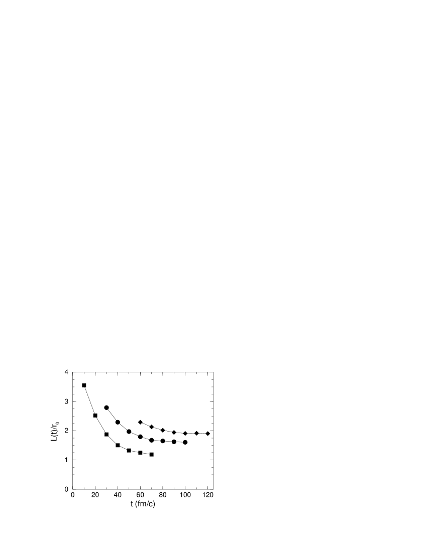
Figure 3: Behavior of the ratio between the length scale and the mean interparticle spacing $L(t)/r_{0}(t)$ for three different values of $\alpha$: squares, $\alpha=10^{-2}\,c/{\rm fm}$; circles, $\alpha=(1/3)10^{-2}\,c/{\rm fm}$; diamonds, $\alpha=(1/6)10^{-2}\,c/{\rm fm}$ .

The ratio $L(t)/r_{0}(t)$ is the only parameter contained in the probability distribution $Y(A,t)$. The formation of the pattern of correlation domains can be viewed as a stationary process starting from the beginning of the plateau of $L(t)/r_{0}(t)$, even if the nuclear system is still expanding. In Fig. 3 the last point ( $t=70\,{\rm fm}/c$ ) of the plot with $\alpha=0.01\,c/{\rm fm}$ should be taken with caution since it lies beyond the estimated range of validity of our calculations.

In the present scenario, once expansion and cooling have brought the bulk of the system within the spinodal zone of the phase diagram, dynamical fluctuations grow with time until they cause the decomposition of the nuclear system. To be more definite, we fix the onset of the phase separation at the instant when the maximum of the variance $\sigma^{2}_{k}(t)$ becomes twice its initial value for $k=0$. In addition, we identify the probability $Y(A,t)$ with the size distribution of the domains containing the liquid phase. Our choice of the instant for the onset of the phase separation is also supported by the observation that this time roughly coincides with the beginning of the plateau observed in the behavior of the ratio $L(t)/r_{0}(t)$. Thus, while fluctuations continue to grow with time, the size distribution $Y(A,t)$ does not change considerably. The times for the beginning of the plateau in the three cases shown in Fig. 3, corresponding to $\alpha=(1,1/3,1/6)10^{-2}~{}c/{\rm fm}$, are $t\sim 50,80,100\>{\rm fm}/c$ respectively.

In order to assess the validity of our approach, we compare the results of our calculations with the corresponding experimental data by identifying the probability $Y(A,t)$ with the distribution of the fragment yield observed in processes of nuclear multifragmentation. The probability $Y(A,t)$ is calculated with the value of $L(t)/r_{0}(t)$ at the plateau. Like in Ref. Mat00 , finite–size and surface effects are not included in our model, consequently a transition from surface to bulk multifragmentation, as suggested recently by the analysis of the ISiS results Beau00 , cannot be described within our approach. However, we expect that our treatment should reliably account for the gross features of the bulk instabilities of nuclear matter, at least at a qualitative level.

Since experimentally the fragments are detected according to their charge, we have to transform $Y(A,t)$ into the corresponding function of $Z$, $Y(Z,t)$. For this purpose, we assume a homogeneous distribution for the charge, $Z=[(1-I)/2]A$, with $I=(N-Z)/A$ and use $I=0.2$, that corresponds to the average asymmetry of the nuclear systems considered.

In Ref. Mat00 it has been shown that the probability $Y(Z)$ can be fitted with good accuracy by a power law $Y(Z)=\,Y_{0}Z^{-\tau_{eff}}$. The parameter $\tau_{eff}$ depends only on the expansion rate of nuclear matter, once the temperature and density at $t=0$ have been fixed. We have taken the initial values $T(0)=6\,{\rm MeV}$ and $\varrho_{0}(0)=0.7\varrho_{eq}$, however, even if the temperature is changed in a rather large interval, the value of the ratio $L(t)/r_{0}(t)$ at the plateau does not change appreciably. In Fig. 4 the effective exponent $\tau_{eff}$ is shown as a function of the radial collective energy per particle, $E_{hy}$, at the break–up of the nuclear system. This energy has a one–to–one correspondence with the parameter $\alpha$, for given initial conditions, and is a more suitable observable than $\alpha$ for a comparison with the experimental data.

Figure 4: Effective exponent of the power law, $Y(Z)=\,Y_{0}Z^{-\tau_{eff}}$, as a function of the collective radial energy per particle at the break–up (the corresponding range of the expansion parameter is $(1/6)10^{-2}\leq\alpha\leq 10^{-2}$).

Figure 4 shows a moderate rise of $\tau_{eff}$ when the energy of the hydrodynamic motion increases. The cause of the expansion can be either dynamical, following an initial compression, or thermal, due to a release of energy in the bulk of the nuclear system from very energetic particles, for instance protons, antiprotons or pions. In both the cases the rapidity of the expansion and, as a consequence, the exponent $\tau_{eff}$ increase with the excitation energy of the nuclear system.

Figure 5: Comparison of fragment distribution $Y(Z)$ calculated for $L(t)/r_{0}(t)=1.3$ ( dot–dashed line ) $1.6$, ( dashed line ) and $2$ ( solid line ) ( $\tau_{eff}=1.65,1.51,1.41$ respectively ), with experimental distributions for the reactions ${}^{129}Xe+Sn$ at $E=32~{}A\,{\rm MeV}$ (triangles) and ${}^{155}Gd+U$ at $E=36~{}A\,{\rm MeV}$ (circles) Fran01 . Both data and curves have been normalized to 1.

Figure 6: Same of Fig. 5, but for the reaction $Xe+Sn$ at $E=50~{}A\,{\rm MeV}$ (diamonds) Ass99 .

In Fig. 5 a comparison is made between the charge distributions predicted by our approach and recent experimental data obtained by the the INDRA Collaboration for ${}^{129}Xe+Sn$ and ${}^{155}Gd+U$ collisions at $E=32~{}A\,{\rm MeV}$ and at $E=36~{}A\,{\rm MeV}$ respectively Fran01 . In Fig. 6, the same comparison is made for $Xe+Sn$ collisions at $E=50~{}A\,{\rm MeV}$ Ass99 . Our calculations have been performed for three different values of the parameter $L(t)/r_{0}(t)$, the corresponding values of the effective exponent $\tau_{eff}$ are given in the legend of Fig. 5. We have normalized both the experimental and the calculated distributions to one in order to perform the comparison on an absolute scale. The agreement between experimental data and our calculated charge distributions is quite satisfactory for $Z<30\div 35$ at the lower incident energies of Fig. 5, and for $Z<20\div 24$ at the higher energy of Fig. 6. For the higher values of $Z$ the observed distributions display a steeper slope than that predicted by our calculations. This faster decrease of the experimental yields should be ascribed to finite–size effects Dag96 that have not been included in our nuclear matter treatment. The comparison also show that experimental data at higher energy are better reproduced with smaller values of the parameter $L(t)/r_{0}(t)$ and correspondingly larger values of $\tau_{eff}$, compared with the values needed to reproduce the data at lower energy. This trend is explained by our scheme, since a growth of the radial collective energy corresponds to an increase of $\tau_{eff}$ ( see Fig. 4 ) and it is reasonable to expect that for central collisions the radial collective motion becomes faster when the incident energy increases.

A further remark about the effective exponent $\tau_{eff}$. It has been experimentally observed that the onset of an expansion in nuclear matter is a signal for a transition from surface–dominated to bulk emission, as expected for a spinodal decomposition, and that the power–law parameter $\tau_{eff}$ grows with excitation energy for expanding nuclear matter Beau99 ; Beau00 . Our results are in qualitative agreement with this observed behavior and so is our estimate of the radial collective energy. However, the experimental values of $\tau_{eff}$ reported in Ref. Beau99 are systematically larger than our values.

IV Summary and Conclusions

We have studied the density fluctuations of expanding nuclear matter within a one–body treatment of nuclear dynamics. In our approach the fluctuations are generated by adding a stochastic term to the mean field and they develop about a local–equlibrium state described by a hydrodynamic expansion. This additional random force is constrained by an extension of the usual fluctuation–dissipation theorem to the case of uniformly expanding systems. In this more general context, we have confirmed the main results obtained in Ref. Mat00 about the particular physical conditions in which a white–noise assumption for the stochastic field can be retained: the density and temperature of the system should be sufficiently close to the borders of the spinodal region in the ($\varrho,T$) plane, so that the limit $\omega/T\ll 1$ gives a reasonable approximation to the density–density response. In this case the equilibrium fluctuations can be adequately described by means of thermodynamic functions.

We have extended the results obtained for the probability distribution of fluctuations in a system at local-equilibrium to unstable situations. This has been done by extrapolating the relevant quantities across the boundary of the spinodal region. Because of the linear approximation used for evaluating the response of the system to the stochastic force, the probability distribution of the fluctuations is Gaussian. The variance of the distribution at a given point in the ($\varrho,T$) plane, strongly depends on the expansion velocity and instabilities are favoured in the case of slower expansions.

In Sec. II.2 we have discussed a procedure to determine the size distribution of the domains containing correlated density fluctuations. This procedure is quite general and can be applied to any Gaussian distribution. For the size distribution we have found an expression similar to that obtained in Ref. Mat00 . It again contains only one parameter, the ratio between the dynamical correlation length and the mean interparticle spacing, $L(t)/r_{0}(t)$. However, in the present case the time behavior of $L(t)$ is mainly determined by the expansion velocity, in other words by the collective energy stored in the excited nuclear system. In particular, the parameter $L(t)/r_{0}(t)$ displays a flat behavior in time after a certain instant that depends on the expansion velocity. Roughly at this time, the amplitude of fluctuations acquires at least twice its initial value and keeps growing. Therefore, the decomposition of the system can be viewed as a quasi stationary process.

In Sec. III we have compared the obtained mass distribution to the yield of intermediate–mass fragments observed in the multifragmentation of heavy nuclei. The comparison with experiment has shown that our approach fairly reproduces the measured charge distributions with $Z<30\div 35$ for collisions at lower energy and with $Z\lesssim 20$ at higher energies. Since we have modeled the system as infinite nuclear matter, we expect to overestimate the number of large fragments. However, it could be worthwhile studying whether and how the finite size effects could become more important with increasing incident energy.

Our approach does account for both the power–law distribution found experimentally and the observed behavior of the effective exponent with the excitation energy, but the calculated exponent is systematically smaller than that determined from experiments. This discrepancy deserves further investigation. *

Appendix A

In this Appendix we briefly discuss the statistical properties of nuclear matter that undergoes the expansion described in Sec. II.1. For this hydrodynamic motion we can assume that in the local reference frame moving with the hydrodynamic velocity ${\bf u}({\bf r},t)$, the physical system is described by the equilibrium density matrix:

$${\widehat{\varrho}}(t)=\frac{1}{Z(t)}e^{\displaystyle-\beta(t)\tilde{H}}\,,$$ (32)

where $Z(t)=Tr{\widehat{\varrho}}(t)$ is the partition function and $\tilde{H}$ is the Hamiltonian in the local reference frame

$$\tilde{H}=\,\sum_{j}\frac{({\hat{\bf p}}_{j}-m{\bf u}({\bf r}_{j},t))^{2}}{2m}+\frac{1}{2}\sum_{i\not=j}V({\bf r}_{i},{\bf r}_{j}).$$ (33)

It can be shown that, for a generic couple of states $|m>$ and $|n>$

$$<m|\tilde{H}|n>=<m|\,e^{i\Sigma_{j}\chi({\bf r}_{j},t)}\,H\,e^{-i\Sigma_{j}\chi({\bf r}_{j},t)}|n>\,,$$

where $\chi({\bf r},t)$ is a gauge function such that $\nabla\chi({\bf r},t)=m{\bf u}({\bf r},t)$. Thus, the statistical density matrix of Eq. (32) is equivalent to

$${\widehat{\varrho}}(t)=\frac{1}{Z(t)}\,e^{i\Sigma_{j}\chi({\bf r}_{j},t)}e^{\displaystyle-\beta(t)H}e^{-i\Sigma_{j}\chi({\bf r}_{j},t)}\,.$$ (34)

Because of the properties of the trace the partition function

$$Z(t)=Tr\,e^{\displaystyle-\beta(t)H}$$

is independent of the velocity field. The density matrix of Eq. (34) reproduces the correct expression both for the collective current and for the density of the hydrodynamic kinetic energy

$$\frac{1}{2}<\sum_{j}\bigg{(}\frac{{\bf p}_{j}}{m}\,\delta({\bf r-r}_{j})+\delta({\bf r-r}_{j})\,\frac{{\bf p}_{j}}{m}\bigg{)}>=\,\varrho_{0}(t){\bf u}({\bf r},t)$$

and

$$<\sum_{j}\bigg{(}\frac{{\bf p}{{}_{j}}^{2}}{2m}\,\delta({\bf r-r}_{j})\bigg{)}>=\,\frac{1}{2}\varrho_{0}(t){\bf u}^{2}({\bf r},t)+{\cal E}_{kin}\,,$$

where ${\cal E}_{kin}$ is the density of the intrinsic kinetic energy.

The observables that commutate with ${\bf r}$ take the same mean value as for a homogeneous medium at equilibrium, having the specific values of density and temperature at a given instant. The same result holds for the equal–time correlation functions of such observables. In particular, for the density fluctuations we obtain

$$<\delta\varrho({\bf r},t)\delta\varrho({\bf r}^{\prime},t)>\,=\frac{1}{Z(t)}Tr\,\delta\varrho({\bf r})\delta\varrho({\bf r}^{\prime})e^{\displaystyle-\beta(t)H}\,.$$ (35)

As far as the correlation functions at different times are concerned, the result of Eq. (11) of Sec. II.1 suggests that, when the collective expansion is slow with respect to the Fermi velocity, these functions depend only on the values of density and temperature of the system at a given instant. In this case, we can reasonably neglect the velocity field $\sum_{j}\chi({\bf r}_{j},t)$ in the expression of the density matrix when evaluating the density correlations. Then we expect that a instantaneous fluctuation–dissipation relation still holds for a medium undergoing a hydrodynamic uniform expansion. In fact, it can be shown that

$$<(\delta\varrho_{\bf k}\delta\varrho_{-\bf k})(\omega)>_{t^{\prime}}=\,-\frac{2}{1-e^{-\beta(t^{\prime})\omega}}{\rm Im}\,D_{k}(\omega,t^{\prime})\,,$$ (36)

where the time Fourier transforms have been evaluated respect to $t-t^{\prime}$. The statistical average is calculated with the density matrix

$${\hat{\varrho}}(t^{\prime})=\frac{1}{Z(t^{\prime})}e^{-\beta(t^{\prime})H}\,.$$

References

- (1) F. Matera and A. Dellafiore, Phys. Rev. C 62, 044611 (2000).
- (2) G.F. Bertsch and S. Das Gupta, Phys. Rep. 160, 189 (1988).
- (3) P. Schuck, R.W. Hasse, J. Jaenicke, C. Grégoire, B. Rémaud, F. Sébille, and E. Suraud, Prog. Part. Nucl. Phys. 22, 181 (1989).
- (4) A. Bonasera, F. Gulminelli, and J. Molitoris, Phys. Rep. 243, 1 (1994).
- (5) B. Tamain and D. Durand, in Proceedings of the International School Trends in Nuclear Physics, 100 years later, Les Houches, Session LXVI, edited by H. Nifenecker, J.–P. Blaizot, G.F. Bertsch, W. Weise, and F. David (North–Holland, Amsterdam,1998), p. 295.
- (6) J. Richert and P. Wagner, Phys. Rep. 350, 3 (2001).
- (7) S. Das Gupta, A. Z. Mekjian, and M. B. Tsang, in Advances in Nuclear Physics, edited by J. W. Negele and E. Vogt (Plenum, New York, 2001), Vol. 26, p. 91.
- (8) B. Borderie, J. Phys. G: Nucl. Part. Phys. 28, R217 (2002).
- (9) S. Ayik and C. Grégoire, Nucl. Phys. A513, 187 (1990).
- (10) J. Randrup and B. Rémaud, Nucl. Phys A514, 339 (1990).
- (11) M. Colonna, Ph. Chomaz, and J. Randrup, Nucl. Phys. A567, 637 (1994).
- (12) M. Colonna, M. Di Toro, A. Guarnera, S. Maccarone, M. Zielinska–Pfabé, and H.H. Wolter, Nucl. Phys. A642 449 (1998).
- (13) G. F. Bertsch and P.J. Siemens, Phys. Lett. B 126, 9 (1983).
- (14) M. Assenard et al., Nucl. Phys. A658, 67 (1999).
- (15) J. D. Frankland et al., Nucl. Phys. A689, 940 (2001).
- (16) L. Beaulieu et al., Phys. Lett. B 463, 159 (1999).
- (17) L. Beaulieu et al., Phys. Rev. Lett. 84, 5971 (2000).
- (18) L.D. Landau and E.M. Lifshitz, Statistical Physics 3rd ed. (Pergamon Press, Oxford, 1982), Pt. 1, Sec. 56.
- (19) M. Brack, C. Guet, and H.–B. Hakansson, Phys. Rep. 123, 275 (1985).
- (20) M. Colonna and Ph. Chomaz, Phys. Rev. C 49, 1908 (1994).
- (21) W.D. Myers and W.J. Swiatecki, Nucl. Phys. 81, 1 (1966).
- (22) M. Colonna, Ph. Chomaz, A. Guarnera, and B. Jacquot, Phys. Rev. C 51, 2671 (1995).
- (23) L. E. Reichl, A Modern Course in Statistical Physics (Edward Arnold Publishers, London, 1980).
- (24) C.W. Gardiner, Handbook of Stochastic Methods (Springer–Verlag, Berlin, 1997), Ch. 4.
- (25) D. Kiderlen and H. Hofmann, Phys. Lett. B 353, 417 (1995); H. Hofmann and D. Kiderlen, Int. J. Mod. Phys. E7, 243 (1998).
- (26) J.D. Gunton, M. San Miguel, and Paramdeep S. Shani, in Phase Transitions and Critical Phenomena, edited by C. Domb and J.L. Lebowitz (Academic Press, London, 1983), Vol. 8, p. 267.
- (27) M. D’Agostino et al., Phys. Lett. B 371, 175 (1996).