Hydrodynamics Near a Chiral Critical Point

Abstract

We introduce a model for the real-time evolution of a relativistic fluid of quarks coupled to non-equilibrium dynamics of the long wavelength (classical) modes of the chiral condensate. We solve the equations of motion numerically in 3+1 space-time dimensions. Starting the evolution at high temperature in the symmetric phase, we study dynamical trajectories that either cross the line of first-order phase transitions or evolve through its critical endpoint. For those cases, we predict the behavior of the azimuthal momentum asymmetry for high-energy heavy-ion collisions at nonzero impact parameter.

I Introduction

The hydrodynamical model is frequently employed to describe multiparticle production processes in hadronic collisions [1]. In particular, it predicts characteristic flow-signatures as “fingerprints” for non-trivial equations of state of hot and dense matter [2]. Such equations of state can occur when the effective potential, obtained by integrating out some degrees of freedom, exhibits features characteristic of a phase transition in thermodynamics [3].

More specifically, if there exist two (or more) collective states with the same free energy but separated by a barrier, then behavior characteristic of a first-order phase transition may emerge. On the other hand, if no free-energy barrier exists, one might expect resemblence to a second-order phase transition. This analogy of interacting quantum field theories with thermodynamics is believed to have played an important role in the evolution of the early universe [4] and is currently being investigated in accelerator experiments by colliding beams of protons and heavy ions [5]. Classical energy flow and hydrodynamic scaling behavior emerges in high-energy inclusive processes [1, 6] and from the real-time evolution of some quantum field theories [7].

In this paper, we extend the hydrodynamical transport model such that phase transitions related to the restoration (or breaking) of some global symmetry can be studied dynamically. In particular, we focus on chiral symmetry breaking at finite temperature [8], for which we shall adopt a relatively simple and tractable phenomenological model, i.e. the Gell-Mann and Levy model [9].

It has been argued [10, 11, 12, 13] that the chiral phase transition for two massless quark flavors is second-order at baryon-chemical potential $\mu_{B}=0$, which then becomes a smooth crossover for small quark masses. On the other hand, a first-order phase transition is predicted for small temperature $T$ and large $\mu_{B}$. If, indeed, there is a smooth crossover for $\mu_{B}=0$ and high $T$, and a first-order transition for small $T$ and high $\mu_{B}$, then the first-order phase transition line in the $(\mu_{B},T)$ plane must end in a second-order critical point. This point was estimated [10] to be at $T\sim 100$ MeV and $\mu_{B}\sim 600$ MeV (see also [12, 13]). More recently, it has been attempted to determine the endpoint of the line of first-order phase transitions from the lattice, using $2+1$ quark flavors on $N_{t}=4$ lattices [14] (see also [15]). Those authors locate the critical point at $T=160\pm 3.5$ MeV and $\mu_{B}=725\pm 35$ MeV. Note, however, that a reliable extrapolation to the continuum limit and to physical pion mass has not been attempted so far.

There is an ongoing experimental effort to detect that chiral critical point in heavy-ion collisions at high energies. Note that both, high temperature and high baryon density are required to have dynamical trajectories in heavy-ion collisions pass reasonably close by the critical point. Some dynamical computations [16] of the energy deposition and baryon stopping process during the initial stage of head-on collisions of large nuclei within semi-realistic multi-fluid dynamical models suggest that the required conditions may be reached in the central region of collisions at $E_{lab}\simeq 20-80$ AGeV on a fixed target, or in the fragmentation regions of collisions at higher energies. However, to our knowledge there has been so far no attempt to describe hydrodynamical expansion of the hot and dense droplet produced initially for dynamical trajectories close to the critical point. This paper represents an attempt in that direction.

II The Model

In this section we shall present our model for the dynamics of a droplet of quarks and antiquarks, starting at high temperature in a state with (approximately) restored chiral symmetry, and evolving towards a state where the symmetry is spontaneously broken. The quarks will be described as a heat bath in local thermal equilibrium that evolves in 3+1 dimensions according to the conservation laws for energy and momentum, i.e. relativistic hydrodynamics. However, the “fluid” of quarks interacts locally with the chiral fields, that is, they can exchange energy and momentum. In turn, the (long wavelength modes of the) fields obey the classical equations of motion which follow from the underlying Lagrangian in the presence of the quarks and anti-quarks. Similar models for the dynamics of quarks coupled to chiral fields were considered in the past. In [17], a background of freely streaming quarks was assumed, and the classical evolution of the chiral fields was discussed. More realistic dynamical descriptions for the quark medium followed shortly, treating them as either a relativistic fluid [18], as also envisaged here, or within classical Vlasov transport theory [19, 20]. Those studies focused on a second-order chiral phase transition, or, in the presence of explicit symmetry breaking, on a smooth crossover. However, it turns out that one can also address first-order chiral phase transitions within the very same model, at least in a phenomenological fashion, by chosing larger quark-field coupling $g$ [21, 22] (see below). Integrating out the quarks then leads to an effective potential exhibiting two degenerate states around $T_{c}$.

Here, we extend the previous work mentioned above, and at the same time shift our focus somewhat. Namely, the early studies were mainly concerned with the dynamical evolution of the long-wavelength chiral fields, and of classical pion production; that is, they mainly adressed issues related to the possiblity of forming “Domains of Disoriented Chiral Condensates” (DCC), as suggested by Rajagopal and Wilczek, and others [23], see also [13, 18, 19, 21]. Our present work puts more emphasis on the dynamics of the heat-bath of quarks, rather than on that of the soft modes of the chiral field. We shall point out qualitative changes in the classical energy-momentum flow of the “fluid” of quarks in the proximity of a chiral critical point, rather than look for “rare phenomena” like DCC formation.

Moreover, refs. [17, 18, 19, 20, 21] all employed the mean field approximation for the chiral fields. Field fluctuations at the phase transition were not considered. As an example, for the first-order phase transition discussed in [21] dynamical bubble nucleation (“boiling”) could not be described, as it requires large coherent thermal field fluctuations from the symmetry restored phase, over the barrier and into the symmetry broken phase (see e.g. [24] for results of such dynamical simulations, and [22] for a computation of bubble nucleation rates from the linear sigma model). Thus, the main improvement here is that we do include a dynamical treatment of field fluctuations in the vicinity of a critical point, and their influence on the dynamical evolution of the quark fluid.

On the technical side, going beyond the mean field approximation requires us to introduce appropriate subtractions in all thermodynamical functions, as explained in appendix A. Moreover, the coupled system of non-linear partial differential equations has to be solved numerically in 3+1 dimensions, without imposing any space-time symmetry assumptions (while [17, 18, 19, 21] all simplified the solution greatly by assuming special symmetries which essentially reduced the problem to 0+1 or 1+1 space-time dimensions). That is because fluctuations break any space-time symmetry that may be obeyed by the mean field, as for example spherical symmetry or symmetry under Lorentz boosts in a particular direction.

As mentioned in the introduction, physically the chiral critical point is expected to occur for some specific values of temperature $T$ and baryon-chemical potential $\mu_{B}$. To simplify the problem and its numerical solution, however, here we rather choose to consider only locally baryon symmetric matter, i.e. equal numbers of quarks and anti-quarks. Instead, we can “shift” the critical point by varying the quark-field coupling constant $g$, that is, by increasing or decreasing the vacuum mass of the constituent quarks. As explained in more detail below, large values for $g$ result in a first-order phase transition, while small $g$ leads to a crossover. For the observables discussed in section III, the qualitative difference between the two realizations of a chiral critical point mentioned above should not matter much. On the other hand, our simplified treatment disables us from studying fluctuations of net baryon charge [26].

In section II A we discuss the effective potential “seen” by the long wavelength modes of the chiral fields in the presence of a heat bath of quarks and anti-quarks. Then, in II B we present our model for the non-equilibrium dynamical treatment of field and fluid evolutions. Some numerical algorithms and details are mentioned briefly in section II C. In section III we present our results and end with a summary and an outlook in section IV.

A Effective Potential

As an effective theory of the chiral symmetry breaking dynamics, we assume the linear $\sigma$-model coupled to two flavors of quarks [9]:

$${\cal L} = \overline{q}\,\left[i\gamma^{\mu}\partial_{\mu}-g(\sigma+\gamma_{5}\vec{\tau}\cdot\vec{\pi})\right]\,q$$ (1)

$$+ \frac{1}{2}\left(\partial_{\mu}\sigma\partial^{\mu}\sigma+\partial_{\mu}\vec{\pi}\partial^{\mu}\vec{\pi}\right)-U(\sigma,\vec{\pi})\quad.$$ (2)

The potential, which exhibits both spontaneously and explicitly broken chiral symmetry, is

$$U(\sigma,\vec{\pi})=\frac{\lambda^{2}}{4}(\sigma^{2}+\vec{\pi}^{2}-{\it v}^{2})^{2}-h_{q}\sigma-U_{0}\quad.$$ (3)

Here $q$ is the constituent-quark field $q=(u,d)$. The scalar field $\sigma$ and the pseudoscalar field $\vec{\pi}=(\pi_{1},\pi_{2},\pi_{3})$ together form a chiral field $\phi_{a}=(\sigma,\vec{\pi})$. The parameters of the Lagrangian are chosen such that chiral $SU_{L}(2)\otimes SU_{R}(2)$ symmetry is spontaneously broken in the vacuum. The vacuum expectation values of the condensates are $\langle\sigma\rangle={\it f}_{\pi}$ and $\langle\vec{\pi}\rangle=0$, where ${\it f}_{\pi}=93$ MeV is the pion decay constant. The explicit symmetry breaking term is due to the non-zero pion mass and is determined by the PCAC relation, which gives $h_{q}=f_{\pi}m_{\pi}^{2}$, where $m_{\pi}=138$ MeV. This leads to $v^{2}=f^{2}_{\pi}-{m^{2}_{\pi}}/{\lambda^{2}}$. The value of $\lambda^{2}=20$ leads to a $\sigma$-mass, $m^{2}_{\sigma}=2\lambda^{2}f^{2}_{\pi}+m^{2}_{\pi}$, approximately equal to 600 MeV. In mean field theory, the purely bosonic part of this Lagrangian exhibits a second-order phase transition [8] if the explicit symmetry breaking term, $h_{q}$, is dropped. For $h_{q}\neq 0$, the transition becomes a smooth crossover from the phase with restored symmetry to that of broken symmetry. The normalization constant $U_{0}$ is chosen such that the potential energy vanishes in the ground state, that is

$$U_{0}=\frac{m_{\pi}^{4}}{4\lambda^{2}}-f_{\pi}^{2}m_{\pi}^{2}~{}.$$ (4)

For $g>0$, the finite-temperature one-loop effective potential also includes a contribution from the quarks. In our phenomenological approach, we shall consider the quarks as a heat bath in (local) thermal equilibrium. Thus, it is possible to integrate them out to obtain the effective potential for the chiral fields in the presence of that bath of quarks. Consider a system of quarks and antiquarks in thermodynamical equilibrium at temperature $T$ and in a volume ${\cal V}$. The grand canonical partition function reads

$${\cal Z}=\int{\cal D}\bar{q}\,{\cal D}q\,{\cal D}\sigma\,{\cal D}\vec{\pi}\;\exp\left[\int_{0}^{1/T}d(it)\int_{\cal V}d^{3}{\vec{x}}\,{\cal L}\right]\,\,.$$ (5)

(Anti-) Periodic boundary conditions for the (fermion) boson fields are implied. In mean-field approximation the chiral fields in the Lagrangian are replaced by their expectation values, which we denote by $\sigma$ and $\vec{\pi}$. Then, up to an overall normalization factor,

$${\cal Z} = {\cal N}_{U}\int{\cal D}\bar{q}\,{\cal D}q\;\exp\Biggl{\{}i\int_{0}^{1/T}dt\int_{\cal V}d^{3}{\vec{x}}$$ (7)

$$\bar{q}\left[i\gamma^{\mu}\partial_{\mu}-g(\sigma+i\gamma_{5}\vec{\tau}\cdot\vec{\pi})\right]q\Biggr{\}}$$

$$= {\cal N}_{U}\,{\rm det}_{p}\Bigl{\{}\bigl{[}p_{\mu}\gamma^{\mu}-g(\sigma+i\gamma_{5}\vec{\tau}\cdot\vec{\pi})\bigr{]}/T\Bigr{\}}\,\,,$$ (8)

where

$${\cal N}_{U}=\exp\left(-\frac{{\cal V}U(\sigma,\vec{\pi})}{T}\right)~{}.$$ (9)

Taking the logarithm of ${\cal Z}$, the determinant of the Dirac operator can be evaluated in the standard fashion [27], and we finally obtain the grand canonical potential

$$-\frac{T}{{\cal V}}\log{\cal Z}=U+\widetilde{V}_{q}(T)~{},$$ (10)

where

$$\widetilde{V}_{q}(T)=-d_{q}\int\frac{d^{3}{\vec{p}}}{(2\pi)^{3}}\left\{E+T\,\log\left[1+e^{{-E}/{T}}\right]\right\}\,\,.$$ (11)

Here, $d_{q}=24$ denotes the color-spin-isospin-baryon charge degeneracy of the quarks. For our purposes, the zero-temperature contribution to $\widetilde{V}_{q}$, i.e. the first term in the integral in (11), can be absorbed into $U$ via a standard renormalization of the bare parameters $\lambda^{2}$ and $v^{2}$. The logarithmic dependence on the renormalization scale is ignored in the following.

Adding the $T=0$ and the finite-$T$ contributions defines our effective potential $V_{\rm eff}$:

$$V_{\rm eff}(\phi_{a},T)\equiv U(\phi_{a})-d_{q}T\int\frac{d^{3}p}{(2\pi)^{3}}\log\left(1+e^{-E/T}\right)\quad.$$ (12)

$V_{\rm eff}$ depends on the order parameter field through the effective mass of the quarks, $m_{q}=g\sqrt{\phi^{2}}\equiv g\sqrt{\sum_{a}\phi_{a}\phi_{a}}$, which enters into the expression for the energy, $E=\sqrt{p^{2}+g^{2}\phi^{2}}$.

In principle, one should also integrate out short wavelength fluctuations of $\phi$, which would lead to an additional contribution to the effective potential (12), see for example [13, 28]. For the present phenomenological analysis, however, the expression (12) is already sufficient in that it exhibits a critical endpoint for some particular value of the coupling constant $g$. Since we do not expect the simple model (2) to be quantitatively reliable anyway, it is not unreasonable to employ the effective potential (12) for a study of qualitative effects near a chiral critical point.

FIG. 1.: The one-loop finite-$T$ effective potential as a function of the scalar field $\sigma$ at $\vec{\pi}=0$. The quark-field coupling constant $g$ is being varied. The curves are labeled by the value for $g$ and by the temperature in MeV in parantheses. The field self-coupling is chosen to be $\lambda^{2}=20$.

We now turn to a discussion of the shape of the effective potential, cf. Fig. 1. For sufficiently small $g$ one still finds the above-mentioned smooth transition between the two phases. At larger coupling to the quarks, however, the effective potential exhibits a first-order phase transition [21]. Along the line of first-order transitions, for temperatures near the critical temperature, $V_{\rm eff}$ displays a local minimum $\sigma=\sigma_{1}(T)\simeq 0$ which is separated by a barrier from another local minimum at $\sigma=\sigma_{2}(T)>0$. (There is another local minimum for negative $\sigma$ which is of higher energy and does not concern us.) These two minima are degenerate at $T=T_{c}$. For example, $g=5.5$ leads to a critical temperature of $T_{c}\simeq 123.3$ MeV. Lowering the value of $g$ leads to a smaller barrier between the two degenerate states. Also, $\sigma_{1}$ approaches $\sigma_{2}$, i.e., the phase transition weakens, and moreover the spinodal temperature approaches $T_{c}$ [22]. At $g_{c}\simeq 3.7$, finally, the barrier disappears, and so the latent heat vanishes. This is the second-order critical point, where the potential about the minimum is flat.

A different possibility of making the $\sigma$-meson much lighter at $T_{c}$ than at $T=0$ is to reduce the self-coupling of the chiral fields [29], $\lambda^{2}$, rather than that to the quarks. For example, one may choose $\lambda^{2}\simeq 2.2$ with the pion decay constant $f_{\pi}$ and vacuum mass $m_{\pi}$ fixed, such that $v^{2}=0$. However, within the present model this also reduces $T_{c}$ significantly, to less than $100$ MeV [22]. Such low $T_{c}$ appear to be excluded by present lattice QCD results [30], and moreover would generate too small thermal fluctuations in the heat bath. Therefore, we keep $\lambda^{2}=20$ fixed throughout the manuscript.

B Coupled Dynamics of Fields and Fluid

The classical equations of motion for the chiral fields are

$$\partial_{\mu}\partial^{\mu}\sigma+\frac{\delta U}{\delta\sigma} = -g\left<\bar{q}q\right>=-g\rho_{s},$$ (13)

$$\partial_{\mu}\partial^{\mu}\vec{\pi}+\frac{\delta U}{\delta\vec{\pi}} = -g\left<\bar{q}\gamma_{5}\vec{\tau}\,q\right>=-g\vec{\rho}_{ps},$$ (14)

where

$$\rho_{s} = \langle\overline{q}q\rangle=g\sigma\,d_{q}\int\frac{{\rm d}^{3}p}{(2\pi)^{3}}\frac{1}{E}f(p)~{},$$ (15)

$$\vec{\rho}_{ps} = \langle\overline{q}\gamma_{5}{\vec{\tau}}q\rangle=g\vec{\pi}\,d_{q}\int\frac{{\rm d}^{3}p}{(2\pi)^{3}}\frac{1}{E}f(p)$$ (16)

are the scalar and pseudoscalar densities generated by the heat bath of quarks and anti-quarks, respectively. The distribution of the quarks and anti-quarks in momentum space is given by the Fermi-Dirac distribution.

The form (14) for the coupling to the heat bath of quarks can be derived from the Lagrange density (2) in mean-field approximation. The energy density of the quarks is given by

$$\left<{\cal H}_{q}\right>=\left<\bar{q}i\partial\!\!\!/q\right>+g\left<\overline{q}\sigma q\right>+g\left<\overline{q}\gamma_{5}\vec{\tau}\cdot\vec{\pi}q\right>~{}.$$ (17)

The finite-$T$ contribution to the equation of motion for the $\sigma$, $\vec{\pi}$ fields is obtained from the variation of the effective potential with respect to $\sigma$ or $\vec{\pi}$, respectively:

$$g\left<\overline{q}q\right> = \frac{\delta\left<{\cal H}_{q}\right>}{\delta\sigma}=\frac{\delta\left<V_{\rm eff}-U\right>}{\delta\sigma}~{},$$ (18)

$$g\left<\overline{q}\gamma_{5}\vec{\tau}\,q\right> = \frac{\delta\left<{\cal H}_{q}\right>}{\delta\vec{\pi}}=\frac{\delta\left<V_{\rm eff}-U\right>}{\delta\vec{\pi}}~{}.$$ (19)

Applying this to the right hand side of equation (12) yields the expressions for the scalar density and the pseudoscalar density as given in (15).

As already mentioned above, we shall assume that the quarks constitute a heat bath in local thermal equilibrium. Thus, their dynamical evolution is determined by the local conservation laws for energy and momentum in relativistic hydrodynamics. For simplicity, we shall further assume that the stress-energy tensor of the quark fluid is of the “perfect fluid” form (corrections could in principle be taken into account in the future along the lines discussed in [31]),

$$T^{\mu\nu}=(e+p)u^{\mu}u^{\nu}-pg^{\mu\nu}~{}.$$ (20)

Here,

$$u^{\mu}\equiv\frac{T^{\mu\nu}u_{\nu}}{\sqrt{u_{\sigma}T^{\sigma\rho}T_{\rho\alpha}u_{\alpha}}}$$ (21)

is the local four-velocity of the fluid. $g^{\mu\nu}={\rm diag}(1,-1,-1,-1)$ is our metric tensor, and so the line element is $ds^{2}=dt^{2}-d\vec{x}^{\,2}$. The time $t$ is measured in the global restframe. Furthermore,

$$e(\phi,T) = \left<{\cal H}_{q}\right>~{},$$ (22)

$$p(\phi,T) = -V_{\rm eff}(\phi,T)+U(\phi_{a})~{},$$ (23)

denote the energy density and the pressure of the quarks at temperature $T$. Note that we do not assume that the chiral fields are in equilibrium with the heat bath of quarks. Hence, both $e$ and $p$ depend explicitly on $\phi=\sqrt{\sigma^{2}+\vec{\pi}^{2}}$. Given an initial condition on some space-like surface, $T^{\mu\nu}$ at any other causally connected space-time point is determined by

$$\partial_{\mu}T^{\mu\nu}=S^{\nu}~{}.$$ (24)

In the absence of interactions between the chiral fields and the quarks, the source term $S^{\nu}$ vanishes, and the energy and the momentum of the quarks,

$$(E,\vec{P})=\int d\sigma_{\mu}T^{\mu\nu}$$ (25)

are conserved:

$$u_{\mu}\partial^{\mu}E=u_{\mu}\partial^{\mu}P^{i}=0~{}.$$ (26)

With interactions turned on, this is obviously not true any longer. Rather, the total energy and momentum of fluid plus fields is the conserved quantity:

$$S^{\nu}=-\partial_{\mu}T^{\mu\nu}_{\phi}~{}.$$ (27)

The stress-energy tensor for the fields can be computed from the Lagrange density in the standard fashion. The effective mass of the quarks, $m_{q}=g\sqrt{\sum_{a}\phi_{a}^{2}}$, is already accounted for in the EoS for the quark fluid, see eqs. (23). Thus, $T^{\mu\nu}_{\phi}$ is the stress-energy tensor of the chiral fields alone:

$$T^{\mu\nu}_{\phi} = \sum\limits_{a}\frac{\partial\left<{\cal L}_{\phi}\right>}{\partial\left(\partial_{\mu}\phi_{a}\right)}\partial^{\nu}\phi_{a}-g^{\mu\nu}\left<{\cal L}_{\phi}\right>$$ (28)

$${\cal L}_{\phi} = \sum\limits_{a}\frac{1}{2}(\partial_{\mu}\phi_{a})(\partial^{\mu}\phi_{a})-U~{}.$$ (29)

Its divergence is given by

$$-\partial_{\mu}T^{\mu\nu}_{\phi} = -\sum\limits_{a}\left\{\partial_{\mu}\partial^{\mu}\phi_{a}+\frac{\delta U}{\delta\phi_{a}}\right\}\partial^{\nu}\phi_{a}$$ (30)

$$= g\rho_{s}\partial^{\nu}\sigma+g\vec{\rho}_{ps}\cdot\partial^{\nu}\vec{\pi}~{}.$$ (31)

In the second step we made use of the equations of motion (14). This is the source term in the continuity equation (24) for the stress energy tensor of the quark fluid. A different derivation based on moments of the classical Vlasov equation for the quarks was given in [17, 18], see also [19].

We emphasize again that we employ eqs. (14) not only to propagate the mean field through the transition but fluctuations as well. The initial condition includes some generic “primordial” spectrum of fluctuations, see section III A, which then evolve in the effective potential generated by the matter fields, i.e. the quarks. Near the critical point, those fluctuations have small effective mass and “spread out” to probe the flat effective potential. Since all field modes are coupled, effectively the fluctuations act as a noise term in the equation of motion for the mean field, similar to the familiar Langevin dynamics [32]; near the phase transition, however, the noise is neither Gaussian (the effective potential is not parabolic) nor Markovian (zero correlation length in time) nor white (zero correlation length in space). Rather, correlation lengths and $n$-point functions of the “noise” are governed by the dynamics of the fluctuations in the effective potential generated by the fluid of quarks, including also effects from the finite size and the relativistic expansion of the system.

C Numerics and Technical Details

We briefly describe how we solved the coupled system (14,24) of partial differential equations in 3+1 space-time dimensions.

We follow the evolution on $t=const$ hypersurfaces, and in a fixed spatial cube of volume $L^{3}$. We discretize three-space in that cube by introducing a $160^{3}$ grid with a spacing of $\Delta x=0.2$ fm (thus, $L=160\times 0.2$ fm=32 fm). On that grid, we solve the hyperbolic continuity equations of fluid dynamics (24) using the so-called phoenical SHASTA flux-corrected transport algorithm with simplified source treatment. It is described and tested in detail in Ref. [33], and we refrain from a discussion here. The time step was chosen as $\Delta t=0.4\Delta x$, as appropriate for the SHASTA [33, 34]. We performed each time step in the standard fashion with $S^{\nu}=0$, then subtracted the sources $S^{\nu}$ from the energy and momentum density in the calculational frame (i.e. the global rest frame of the fluid). Finally, from $T^{00}$, $T^{0i}$ and the EoS $p=p(e,\phi_{a})$ we solved for the velocity of the local restframe (LRF) of each cell, and for the energy density $e$ of the fluid in the LRF. Such a treatment of sources in the continuity equations for energy and momentum proved to work well in relativistic multi-fluid dynamics [16, 34], where one encounters a similar equation due to interactions between various fluids. The boundary conditions at the edge of the computational grid are such that the fluid simply streams out when reaching the boundary. This can be monitored by checking the conservation of the total energy as a function of time.

Regarding the fields, we solve the classical equations of motion using a staggered leap-frog algorithm with second-order accuracy in time, see for example Ref. [35]. The non-linear wave-equations (14) are split into two coupled first-order equations (in time) by considering separately the field $\phi_{a}$ and its canonically conjugate field $d\phi_{a}/dt$. For this algorithm, the time step for propagation of the fields has to be chosen smaller than that for propagation of the fluid. In practice, we found that $\Delta t=0.1\Delta x$ gave reasonable accuracy. As the time step for propagation of the fluid was chosen to be four times larger, the fields where propagated for four consecutive steps, with the fluid kept “frozen”, followed by one single step for the fluid. Spatial gradients of the fields where set to zero at the edges of the computational grid, rather than employing periodic boundary conditions. The spatial derivatives in the equations of motion for the fields (14) where discretized to second order accuracy in the grid spacing to match the second order accuracy in time. We employed the same small grid spacing $\Delta x=0.3$ fm as for the fluid. Although the mean fields vary on a larger scale, it is important to allow for non-linear amplification of harder fluctuations which can couple to the soft modes and affect the dynamical relaxation to the vacuum state with broken symmetry, see for example [36] and [37].

For the fluid, one needs to introduce nine 3d spatial grids, for $e$, $p$, $T^{0\mu}$, and $\vec{u}\,$. In addition, one needs two more 3d grids for each field component, namely for $\phi_{a}$ and $d\phi_{a}/dt$. To save computational resources, we have therefore decided to neglect the pion field altogether, i.e., to set it to zero everywhere in the forward light cone. Thus, only the $\sigma$-field is considered in the actual computations described below. However, this represents a minor restriction only, since we focus here on the bulk evolution of the quark fluid rather than on fluctuation observables or coherent pion production from the decay of a classical pion field. (Coherent pion production is known to contribute a small fraction of the total pion yield only [18, 19, 21, 23, 38]. Incoherent particle production from the decay of the fluid by far dominates, if no kinematic cuts are applied.)

III Results

Having formulated our model, we now proceed to show some specific examples of numerical solutions. In particular, we would like to examine whether the dynamical evolution changes as one crosses the chiral critical point.

A Initial Condition

As an example, we employ the following initial conditions for the results described below. Of course, one could employ more refined initial conditions and “tune” them such as to reproduce various aspects of the final state, which in principle could be compared to experimental data. At present, our more modest goal is to illustrate qualitative effects originating from the phase transition. The initial conditions are meant to provide a semi-realistic parameterization of the hot fireball created in a high-energy heavy-ion collision.

At time $t=0$, the distribution of energy density for the quarks is taken to be uniform in the $z$-direction (with length $2l_{z}=12$ fm) and ellipsoidal in the $x-y$-plane:

$$e(t=0,\vec{x})=\left\{\begin{array}[]{r@{\quad: \quad}l}e_{\rm eq}&x^{2}b^{2}+y^{2}a^{2}<(ab)^{2}\wedge z<l_{z}\\ 0&x^{2}b^{2}+y^{2}a^{2}>(ab)^{2}\vee z>l_{z}\end{array}\right.\quad,$$ (32)

where $e_{\rm eq}$ denotes the equilibrium value of the energy density taken at a temperature of $T_{i}\approx 160$ MeV. In our calculation we choose $a=r_{A}-\tilde{b}/2$ and $b=\sqrt{r_{A}^{2}-\tilde{b}^{2}/4}$, where $\tilde{b}$ denotes the impact parameter of two nuclei with radius $r_{A}$ (below, we choose $r_{A}=6.5$ fm and $\tilde{b}=6$ fm). Thus, the ellipsoidal shape resembles the almond shaped overlap of two colliding nuclei. The $\Theta$-function distribution of the initial energy density is evidently somewhat unrealistic; a smoother distribution with non-zero surface thickness would be more realistic and perhaps affect the results somewhat. However, as already mentioned above, here we do not aim at quantitative fits to experimental data but at illustrating qualitative effects related to the shape of the effective potential in the transition region.

The collective longitudinal velocity of the fluid of quarks is assumed to rise linearly with $z$: $v_{z}(t=0,\vec{x})\propto z/l_{z}\cdot v_{max}$, where $v_{max}=0.2$ . The transverse components of $\vec{v}$ are set to zero at $t=0$.

Our initial conditions for the chiral fields are

$$\sigma(t=0,\vec{x}) = \delta\sigma(\vec{x})+f_{\pi}+$$ (35)

$${}(-f_{\pi}+\sigma_{\rm eq})\cdot\left[1+\exp\left(\frac{\tilde{r}-\tilde{R}}{\tilde{a}}\right)\right]^{-1}$$

$${}\cdot\left[1+\exp\left(\frac{|z|-l_{z}}{\tilde{a}}\right)\right]^{-1}~{},$$

$$\vec{\pi}(t=0,\vec{x}) = \delta\vec{\pi}(\vec{x})\,,$$ (36)

where $\tilde{r}=\sqrt{x^{2}+y^{2}}$,

$$\tilde{R}=\left\{\begin{array}[]{r@{\quad: \quad}l}\displaystyle\frac{ab\tilde{r}}{\sqrt{b^{2}x^{2}+a^{2}y^{2}}}&\tilde{r}\neq 0\\ a&\tilde{r}=0\end{array}\right.\quad,$$ (37)

and $\tilde{a}=0.3$ fm is the surface thickness of this Woods-Saxon like distribution. Here $\sigma_{\rm eq}\approx 0$ is the value of the $\sigma$ field corresponding to $e_{\rm eq}$. Thus, the chiral condensate nearly vanishes at the center, where the energy density of the quarks is large, and then quickly interpolates to $f_{\pi}$ where the matter density is low.

$\delta\sigma(\vec{x})$ and $\delta\vec{\pi}(\vec{x})$ represent the initial random fluctuations of the fields. Our focus at this stage is on how those “primordial” fluctuations evolve through the phase transition (or crossover) and how they affect the hydrodynamic expansion of the thermalized matter fields (the fluid). Thus, for a first qualitative analysis we do not rely on additional physics input for the primordial fluctuations but rather chose a generic Gaussian distribution,

$$P[\delta\phi_{a}]\propto\exp\left(-\delta\phi_{a}^{2}/2\left<\delta\phi_{a}^{2}\right>\right)~{},$$ (38)

with the variance $\left<\delta\phi_{a}^{2}\right>$ left as a free parameter. (Here, no summation over the index $a$ (internal space) is carried out.) We performed simulations with $\surd\left<\delta\phi_{0}^{2}\right>\equiv\surd\left<\delta\sigma^{2}\right>=v/3$. Such fluctuations are large enough to probe the barrier of the effective potential in case of a first order transition, or the flat region close to the critical endpoint (Fig. 1). On the other hand, they are sufficiently small to allow for a one-loop subtraction of their contribution to the effective potential, as described in appendix A.

The time derivatives of the fields where set to zero at $t=0$, with no fluctuations. As already mentioned in section II C, the actual numerical computations described below were performed with $\delta\vec{\pi}\equiv 0$, i.e. $\left<\delta\phi_{1,2,3}^{2}\right>=0$.

One must further take into account that the field fluctuations are correlated over some space-like distance $\xi\simeq 1$ fm. This is a physical scale which is present in the initial conditions; if one simply picks random fluctuations at each point of the grid, the correlation length will instead be given by the artificial numerical discretization scale $\Delta x$.

In practice, a useful and simple procedure to implement physical correlations in the initial condition is as follows. First, at each point of the grid one samples the distribution (38) at random. Then, one smoothly sweeps a ”sliding window” of linear size $\xi=n\Delta x$ over the grid and averages the fields:

$$\phi_{a}^{\prime}(\vec{x}) = \frac{1}{n^{3}}$$ (40)

$$\times\sum\limits_{i,j,k=0..n-1}\phi_{a}(\vec{x}+i\Delta x\vec{e}_{1}+j\Delta x\vec{e}_{2}+k\Delta x\vec{e}_{3})~{}.$$

Here, $\vec{e}_{1}$, $\vec{e}_{2}$, $\vec{e}_{3}$ define a global cartesian orthonormal basis, and $\vec{x}=1\vec{e}_{1}+1\vec{e}_{2}+1\vec{e}_{3}$, $1\vec{e}_{1}+1\vec{e}_{2}+2\vec{e}_{3}$, $\cdots$, is the sequence of grid points. Clearly, the above averaging procedure “cools” the fluctuations, in that $\langle\delta\phi_{a}^{\prime 2}\rangle\neq\langle\delta\phi_{a}^{2}\rangle$. In particular, in the continuum limit $\Delta x\to 0$ with $\xi=n\Delta x$ held constant, one of course finds that $\langle\delta\phi_{a}^{\prime 2}\rangle\to 0$ for the distribution (38). Therefore, in a final sweep over the grid one has to rescale the fields at each grid point by

$$\phi_{a}^{\prime\prime}(\vec{x})=\phi_{a}^{\prime}(\vec{x})\sqrt{\frac{\left<\delta\phi_{a}^{2}\right>}{\left<\delta\phi_{a}^{\prime 2}\right>}}~{}.$$ (41)

This procedure leads to an initial field configuration that exhibits both the proper physical correlation length and the desired fluctuations. Moreover, it prevents the initial energy density from field gradients to grow like $1/\Delta x^{\,2}$.

B Numerical Solution

In the following we consider both a first order phase transition corresponding to $g=5.5$, as well as the critical point at $g=3.7$.

Figs. 2 and 3 depict the time evolution of the $\sigma$ field along the $x$-axis and the $y$-axis, respectively. At $t=0$ the field within the hot region has small amplitude, corresponding to the chiral symmetry restored phase. That region is surrounded by the physical vacuum with $\langle\sigma\rangle=f_{\pi}=93$ MeV.

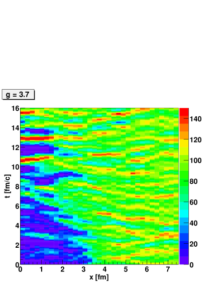
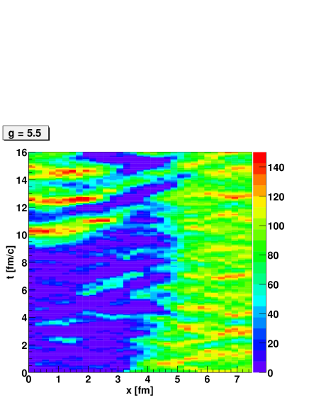
FIG. 2.: Space-time evolution of the chiral field along the $x$-axis at $y=z=0$. Dark regions correspond to small field amplitudes (symmetric phase), light regions to large amplitudes (broken phase). The scale on the right specifies the field amplitude in MeV.

For the first order phase transition ($g=5.5$) a barrier separates the two degenerate minima of the effective potential (Fig. 1) at $T_{c}$. Figs. 2 and 3 show that this barrier leads to a rather well-defined surface in coordinate space, separating the vacuum from the symmetric phase. For the above-mentioned initial conditions, the fluctuations are not strong enough for the field to easily overcome the barrier. Nevertheless, one can observe dynamical fluctuations into the broken symmetry state, e.g. at $x\simeq 1$ fm and $t\simeq 2-4$ fm/c, which however collapse again. Our dynamical results agree with previous arguments that nucleation is a slow process on the time scale of heavy-ion collisions, and so the Gibbs phase equilibrium is not established dynamically [21, 22, 24, 39]. At time $t\simeq 9$ fm the phase transition occurs spontaneously “in an instant”, that is, on a space-like surface which can clearly be seen in Figs. 2 and 3. A “bubble” of the symmetric phase survives at $x\simeq 3$ fm for a long time.

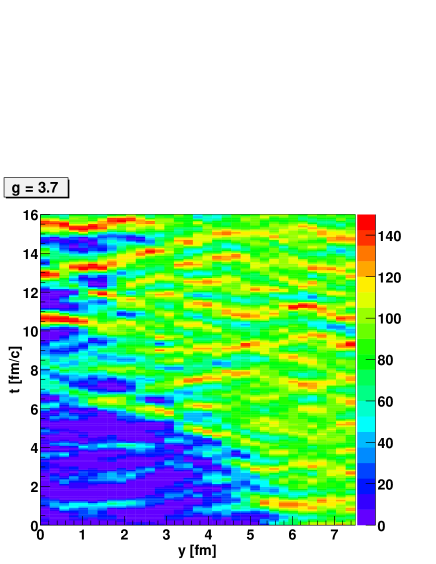
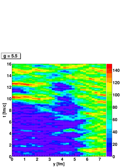
FIG. 3.: Space-time evolution of the chiral field along the $y$-axis at $x=z=0$.

The picture is rather different for the transition at the critical point, i.e. $g=3.7$. Here, the barrier between the degenerate minima vanishes and the potential is flat. As is evident, there are no clear surfaces separating either the vacuum from the center or high-density bubbles (or “droplets”) from their surrounding. Due to the flatness of the potential, near the center the field performs large-amplitude oscillations (from $\sigma\sim 0$ to $\sigma>f_{\pi}$) for a long time; they extend in space over distances $\approx 1-3$ fm (e.g. at $t\approx 9$, 12, and 14 fm/c in Fig. 2), which is not much less than the initial size of the hot region. Figure 4 shows a histogram of the field distribution at the center ($\sqrt{x^{2}+y^{2}+z^{2}}<2~{}fm$). One observes that the distribution broadens from $t=4$ fm to $t=10$ fm, and then narrows again at later times after the transition to the broken phase occured. Also, notice that the distributions at $t=4$ fm and $t=14$ fm are well described by Gaussians, i.e. the effective potential is essentially parabolic, while for $t=10$ fm there are visible deviations from a simple Gaussian.

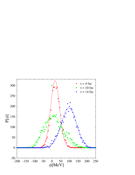
FIG. 4.: Histogram of the field distribution at the center for three different times. Lines represent Gaussian fits with standard deviations 25 MeV (t=4 fm), 53 MeV (t=10 fm), and 43 MeV (t=14 fm).

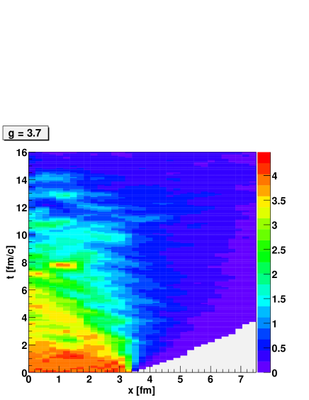
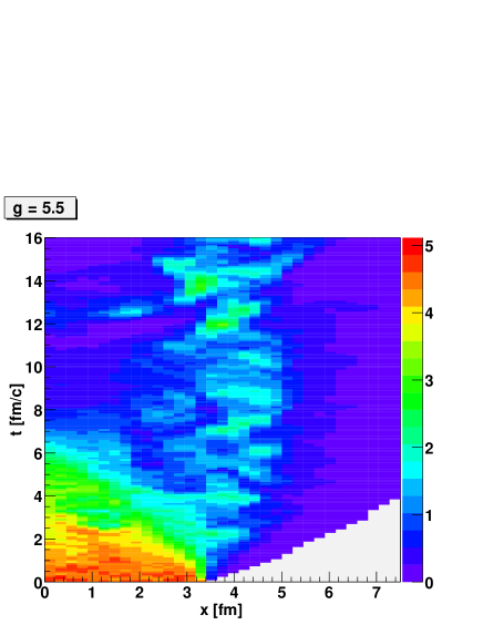
FIG. 5.: Space-time evolution of the fluid energy density along the $x$-axis at $y=z=0$. The scale on the right specifies the energy density in units of nuclear matter density $e_{0}\approx 150$ MeV/fm³.

The time evolution of the local rest-frame energy density $e$ of the quarks is shown in Figs. 5, 6. Again we see large-scale structures for the first order phase transition ($g=5.5$), while the energy density is rather homogeneous on large time and distance scales if the expansion trajectory goes through the critical endpoint. For the first-order transition, quarks can be “trapped” in droplets with $\sigma\sim 0$ (the minimum of the effective potential where the symmetry is restored) because the mass barrier can keep them from escaping. The droplet of high-density matter at $x\simeq 3$ fm and $t\simeq 12-16$ fm/c can easily be associated to the region of nearly vanishing chiral scalar field from Fig. 2. Eventually, that region must perform the transition to the symmetry broken state, either by a strong thermal fluctuation or when reaching the spinodal point. At the spinodal, the system is as far from local thermal equilibrium as it can get, and the “roll-down” of the order parameter field to the global minimum of the potential can influence the collective expansion of the quark fluid.

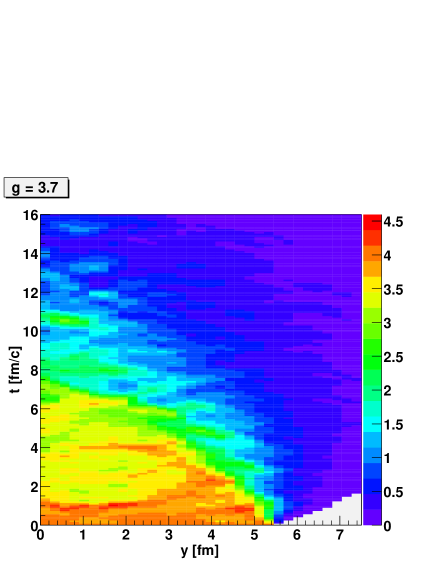
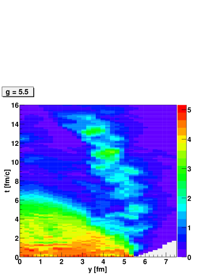
FIG. 6.: Space-time evolution of the energy density along the $y$-axis at $x=z=0$.

Note that the energy density at the center drops more rapidly for the first-order transition than near the critical endpoint. This has consequences for the build-up of azimuthally asymmetric flow, as we shall discuss below.

Fig. 7 depicts the time evolution of the azimuthal momentum anisotropy [40]

$$\epsilon_{p}=\frac{\langle T_{xx}-T_{yy}\rangle}{\langle T_{xx}+T_{yy}\rangle}~{},$$ (42)

where the averages of the stress-energy tensor of the fluid are taken at fixed time:

$$\langle T_{ij}\rangle(t)\equiv\int d^{3}x\,T_{ij}(t,\vec{x})~{}.$$ (43)

Also, we average over a few initial field configurations, which gave similar results for $\epsilon_{p}(t)$, though.

For the above-mentioned initial conditions the energy-momentum tensor is symmetric, and so $\epsilon_{p}=0$ at $t=0$ (this might be different in more realistic treatments [41]). Pressure gradients in $x-$ and $y-$ directions are different, though. Therefore, the acceleration of the fluid is stronger in the reaction ($x-z$) plane than out of plane, leading to a nonzero azimuthal asymmetry $\epsilon_{p}>0$ at times $t>0$. The asymmetry first grows nearly linearly with time but saturates when the asymmetry of the energy density and of the pressure gradients becomes small. As explained above (Figs. 5, 6), this happens earlier for a first-order transition than for trajectories near the chiral critical endpoint. This is then reflected in the final value of $\epsilon_{p}$. We stress that the more rapid saturation of the azimuthal asymmetry in case of a first-order transition is not in contradiction to the fact that hot (high-energy density) “droplets” survive for rather long times, as seen in the figures. Rather, such “droplets” typically turn out to be more or less rotationally symmetric, or at least exhibit deformations which are uncorrelated to the reaction plane (the $x-z$ plane in our case). Thus, they tend to reduce the average azimuthal asymmetry of the energy-momentum tensor.

For comparison, in Fig. 7 we also show the result for an equilibrium first-order phase transition. Here, the equations of motion for the chiral fields, eqs. (14) are not solved but rather the $\sigma$-field is required to populate the (global) minimum of the effective potential,

$$\frac{\delta V_{\rm eff}}{\delta\sigma} = 0~{},$$ (44)

$$\frac{\delta^{2}V_{\rm eff}}{\delta\sigma^{2}} > 0~{}.$$ (45)

That is, the chiral field is in equilibrium with the quark-antiquark fluid and does not exhibit any explicit space-time dependence. At $T_{c}$, where two degenerate minima exist, one performs the usual Maxwell-Gibbs construction to determine the fractions of the total volume occupied by matter in the symmetric and the broken symmetry phases, respectively. Evidently, for the above-mentioned initial conditions the equilibrium phase transition leads to nearly the same azimuthal asymmetry of $T^{ij}$ as for the cross over. Therefore, it is indeed the non-equilibrium real-time dynamics (field fluctuations over the free-energy barrier) that is responsible for the observed reduction of $\epsilon_{p}$ in the regime of first-order chiral phase transitions.

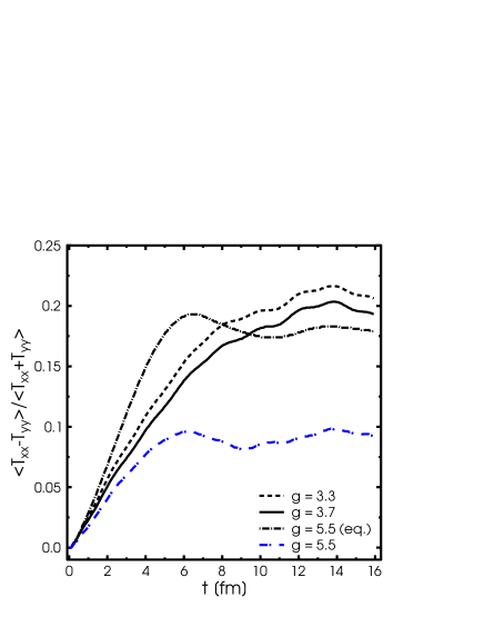
FIG. 7.: Time evolution of the momentum anisotropy for a cross over ($g=3.3$), a second-order phase transition at the critical point ($g=3.7$), and a first order phase transition ($g=5.5$) in or out of equilibrium.

IV Summary and Outlook

In summary, we have introduced a simple phenomenological description of the non-equilibrium real-time dynamics of the chiral phase transition in an expanding (relativistic) fluid of quarks. More precisely, we coupled the linear sigma model, which describes the dynamics of the long-wavelength modes of the chiral order parameter field, to the hydrodynamical evolution of a system of quarks. The chiral field(s) evolve according to the finite-temperature effective potential that is generated by integrating out the quarks from the Lagrangian; in turn, the field(s) determine the effective quark mass (i.e. the equation of state of the quark fluid) dynamically.

The above model exhibits a first order phase transition for large $g$, which is the quark-field coupling constant. The line of first order transitions ends in a critical point when $g$ is lowered, i.e. the transition turns into a cross over for smaller couplings. Thus, by varying $g$ one can qualitatively compare the hydrodynamic expansion pattern of the quark fluid for dynamical trajectories that cross the line of first order transitions to that obtained in the cross over regime.

We have obtained numerical solutions in 3+1 space-time dimensions, using simple initial conditions that might be appropriate for relativistic heavy-ion collisions. The hydrodynamical expansion pattern clearly depends on the structure of the effective potential. For trajectories in the cross over regime or near the critical endpoint the overall bulk dynamics is found to be rather “smooth”, in that the space-time distribution of the energy density of the fluid is not affected very much by the fluctuations of the order parameter field. In the absence of a latent heat, the energy density can not jump much between regions where the field amplitude is different.

In contrast, if the effective potential exhibits a barrier between the symmetry restored and broken phases, respectively, we do see that large-scale structures are formed dynamically, e.g. “droplets” of the symmetric phase may survive for rather long times before becoming mechanically unstable (at the spinodal). In that sense, the overall time scale is longer for trajectories crossing the line of first order transitions. Nevertheless, typically such structures are not correlated to the reaction plane; thus, the direct correspondence of spatial anisotropies in the initial condition to momentum-space anisotropies in the final state predicted by equilibrium hydrodynamics (that is, when the phase transition is not treated dynamically but modelled by a Maxwell-Gibbs construction) is weakened. For example, we find much smaller momentum-space anisotropy for a dynamical first-order transition than for a trajectory through the chiral critical endpoint (for the same initial condition). This could be a very useful prediction with regard to the experimental search for the chiral critical endpoint of QCD in heavy-ion collisions at the BNL-AGS, the CERN-SPS and the envisaged new GSI heavy-ion accelerator. Until now, experiments focused on fluctuation observables, but inclusive observables usually are much easier to analyze accurately.

In the future, we intend to scrutinize other inclusive observables as to their sensitivity to non-equilibrium effects from phase transitions. Of course, there is also plenty of room to improve on the model in order to obtain more quantitative predictions. The present paper represents a first step towards an actual real-time description of the chiral phase transition on either side of the critical endpoint in expanding relativistic fluids with realistic 3+1d geometries.
Note added: After this manuscript was submitted for publication the NA49 collaboration published the elliptic flow at $E_{\rm lab}=40A$ GeV [42]. From Fig. 24 of that publication, the dependence of $v_{2}$ on $\log\sqrt{s}$ is approximately linear. However, the ”natural” scale for $v_{2}$ is set by $\langle p_{\rm t}\rangle$, not $\log\sqrt{s}$, as pointed out by Snellings [43]. Indeed, at high energies the differential $v_{2}(p_{\rm t})$ of charged hadrons is approximately proportional to $p_{\rm t}$, such that the averaged $v_{2}\propto\langle p_{\rm t}\rangle$. In fact, for mid-central collisions $v_{2}$ increases from $\approx 3\%$ at top SPS energy ($\sqrt{s}=18A$ GeV) to $\approx 4.5\%$ at RHIC energy ($\sqrt{s}=130A$ GeV). When scaled by the average transverse momentum, though, the elliptic flow in that energy regime is nearly constant [43]. To scrutinze deviations from the ”natural” scaling $v_{2}\propto\langle p_{\rm t}\rangle$, we plot the excitation function of $v_{2}/\langle p_{\rm t}\rangle$ in Fig. 8.

FIG. 8.: Excitation function of $v_{2}/\langle p_{\rm t}\rangle$ of negatively charged particles in mid-central collisions from top AGS to RHIC energy. Data for $v_{2}$ are taken from Fig. 24 in [42] and $\langle p_{\rm t}\rangle$ from [44, 45, 46, 47].

One observes that, as already mentioned above, the data is compatible with no energy (or $\langle p_{\rm t}\rangle$) dependence above top SPS energy. Clearly, there is a systematic drop of $v_{2}$ relative to $\langle p_{\rm t}\rangle$ towards lower energies. For instance, at $E_{\rm lab}=40A$ GeV corresponding to $\langle p_{\rm t}\rangle\approx 350$ MeV, $v_{2}/\langle p_{\rm t}\rangle$ is lower by about two standard deviations than at higher energies. Qualitatively, this interesting behavior is similar to the reduction of the azimuthal momentum asymmetry, predicted above, caused by crossing the second order critical point into the regime of first order phase transitions. Additional studies of “conventional” non-equilibrium effects unrelated to a phase transition are certainly required, however, before firm conclusions can be drawn.

A Subtracting Initial Fluctuations

In section II A we discussed our phenomenological ansatz for the effective potential for the long wavelength modes of the chiral fields, as generated by the heat bath of quarks. Formally, it is obtained from the Lagrangian by integrating out the quarks to one loop.

Our main objective here is to study dynamically fluctuations of the chiral order parameter (or effects generated by those fluctuations) in the vicinity of the chiral critical point as the system makes the transition to broken chiral symmetry at low temperature. Thus, we have to allow for primordial fluctuations of the chiral fields, also. However, those fluctuations of the fields at time $t=0$ will of course also contribute to the effective potential and “distort” its shape. In order to restore our original choice for $V_{\rm eff}$ from eq. (12), and thus ensure the correct dynamics for the long-wavelength modes, we have to introduce appropriate subtractions.

The procedure is as follows. The scalar and pseudoscalar densities are given by eqs. (16). They depend explicitly on the value of the fields $\phi_{a}$, which we formally separate into short and long wavelengths:

$$\phi_{a}(x)=\left<\phi_{a}\right>+\delta\phi_{a}(x)~{}.$$ (A1)

Here, $\langle\cdot\rangle$ denotes a spatial average over a volume large enough for the fluctuations to average out:

$$\left<\delta\phi_{a}\right>=0~{}.$$ (A2)

The linear dimension of that volume will be given by the wavelength of the soft modes of interest.

We now substitute (A1) into eqs. (16) and perform an expansion up to second order in $\delta\phi_{a}(x)$. We then perform the averaging over the fluctuations with the distribution (38) and obtain

$$\left<\rho_{s}\right> = \rho_{s}(\left<\phi\right>)$$ (A3)

$$+ \frac{1}{2}g\sigma\,d_{q}\int\frac{{\rm d}^{3}k}{(2\pi)^{3}}\biggl{\{}\biggr{.}$$ (A8)

$$\sum\limits_{a}\left<\delta\phi_{a}^{2}\right>\left[-\frac{g^{2}f(k)}{E^{2}T}\left(\frac{T}{E}+f(k)e^{E/T}\right)\right.$$

$$\;\;\;+\;\frac{g^{4}\phi_{a}^{2}}{E^{3}T^{2}}f(k)\left(2f^{2}(k)e^{2E/T}-f(k)e^{E/T}\right.$$

$$\;\;\;+\left.\left.3\frac{T}{E}f(k)e^{E/T}+3\frac{T^{2}}{E^{2}}\right)\right]$$

$$-\left.2\left<\delta\sigma^{2}\right>\frac{g^{2}f(k)}{E^{2}T}\left(\frac{T}{E}+f(k)e^{E/T}\right)\right\}$$

Here, $\left<\delta\phi^{2}\right>\equiv\sum_{a}\left<\delta\phi_{a}\delta\phi_{a}\right>$ is the variance of the fluctuations in the initial condition, i.e. at the initial time $t=0$, summed over internal quantum numbers. We made use of the fact that the fluctuations (38) are diagonal in internal space, i.e. $\left<\delta\phi_{a}\delta\phi_{b}\right>=0$ if $a\neq b$. The second term is the additional contribution seen by the long wavelength modes $\left<\phi_{a}\right>$, which is due to the fluctuations. To restore the original effective potential, we have to subtract that term, i.e. redefine the scalar density as

$$\rho_{s}(\phi,T) = g\sigma\,d_{q}\int\frac{{\rm d}^{3}k}{(2\pi)^{3}}\frac{1}{E}f(k)$$ (A9)

$$- \frac{1}{2}g\sigma\,d_{q}\int\frac{{\rm d}^{3}k}{(2\pi)^{3}}\biggl{\{}\biggr{.}$$ (A14)

$$\sum\limits_{a}\left<\delta\phi_{a}^{2}\right>\left[-\frac{g^{2}f(k)}{E^{2}T}\left(\frac{T}{E}+f(k)e^{E/T}\right)\right.$$

$$\;\;\;+\;\frac{g^{4}\phi_{a}^{2}}{E^{3}T^{2}}f(k)\left(2f^{2}(k)e^{2E/T}-f(k)e^{E/T}\right.$$

$$\;\;\;+\left.\left.3\frac{T}{E}f(k)e^{E/T}+3\frac{T^{2}}{E^{2}}\right)\right]$$

$$-\left.2\left<\delta\sigma^{2}\right>\frac{g^{2}f(k)}{E^{2}T}\left(\frac{T}{E}+f(k)e^{E/T}\right)\right\}$$

This expression has to be substituted for $\rho_{s}$ on the right-hand-side of the equation of motion (14). The subtracted term cancels the “distortion” of the scalar density caused by using the local values $\sigma(x)$, $\vec{\pi}(x)$ for the fields, rather than their long-wavelength components $\langle\sigma(x)\rangle$, $\langle\vec{\pi}(x)\rangle$.

Along the same lines one derives the following expressions for the fluctuation-subtracted pseudo-scalar density, and for the pressure of the quarks:

$$\vec{\rho}_{\rm ps}(\phi,T) = g\vec{\pi}\,d_{q}\int\frac{{\rm d}^{3}k}{(2\pi)^{3}}\frac{1}{E}f(k)$$ (A15)

$$- \frac{1}{2}g\vec{\pi}\,d_{q}\int\frac{{\rm d}^{3}k}{(2\pi)^{3}}\biggl{\{}\biggr{.}$$ (A20)

$$\sum\limits_{a}\left<\delta\phi_{a}^{2}\right>\left[-\frac{g^{2}f(k)}{E^{2}T}\left(\frac{T}{E}+f(k)e^{E/T}\right)\right.$$

$$\;\;\;+\;\frac{g^{4}\phi_{a}^{2}}{E^{3}T^{2}}f(k)\left(2f^{2}(k)e^{2E/T}-f(k)e^{E/T}\right.$$

$$\;\;\;+\left.\left.3\frac{T}{E}f(k)e^{E/T}+3\frac{T^{2}}{E^{2}}\right)\right]$$

$$-\left.2\left<\delta\vec{\pi}^{2}\right>\frac{g^{2}f(k)}{E^{2}T}\left(\frac{T}{E}+f(k)e^{E/T}\right)\right\}$$

$$p(\phi,T) = d_{q}\int\frac{{\rm d}^{3}k}{(2\pi)^{3}}\,T\log\left(1+e^{-E/T}\right)$$ (A21)

$$- \frac{1}{2}\sum\limits_{a}\left<\delta\phi_{a}^{2}\right>\left\{-\frac{g^{2}f(k)}{E}\right.$$ (A22)

$$+ \left.\frac{g^{4}\phi_{a}^{2}}{E^{3}T}f(k)\left[T+E-Ef(k)\right]\right\}~{}.$$ (A23)

One can verify that the identities $g\rho_{s}=-\delta p/\delta\sigma$ and $g\rho_{ps}=-\delta p/\delta\vec{\pi}$ are satisfied, as it should be.

At fixed values for the fields, the energy density of the quarks at a temperature $T$ is given by

$$e(\phi,T)=T\frac{\partial p(\phi,T)}{\partial T}-p(\phi,T)~{}.$$ (A24)

Using the expression for the fluctuation-subtracted pressure given above one obtains

$$e(\phi,T) = d_{q}\int\frac{d^{3}k}{(2\pi)^{3}}Ef(k)$$ (A25)

$$- \frac{1}{2}\sum\limits_{a}\left<\delta\phi_{a}^{2}\right>\left\{\frac{g^{2}f(k)}{ET}\left[T-Ef(k)e^{E/T}\right]\right.$$ (A26)

$$- \frac{g^{4}\phi_{a}^{2}}{E^{3}T}f(k)\left[T+E-Ef(k)\right]$$ (A27)

$$+ \left.\frac{g^{4}\phi^{2}_{a}}{ET^{2}}f^{2}(k)e^{E/T}\tanh\left(\frac{E}{2T}\right)\right\}$$ (A28)

The source term (27) changes due to the fluctuations and one has to use the modified scalar (A9) and pseudoscalar (A15) densities, respectively.

To second order in the fluctuations, the self-interaction of the chiral fields is renormalized as

$$U(\phi_{a}) = \frac{\lambda^{2}}{4}\left(\sigma^{2}+\vec{\pi}^{2}-{\it v}^{2}\right)^{2}-h_{q}\sigma-U_{0}$$ (A29)

$$- \frac{1}{2}\sum\limits_{a}\left<\delta\phi_{a}^{2}\right>\lambda^{2}\left(2\phi_{a}^{2}+\sigma^{2}+\vec{\pi}^{2}-{\it v}^{2}\right)$$ (A30)

The above expressions for $U(\phi_{a})$, $\rho_{s}$, $\vec{\rho}_{ps}$, $e$, and $p$ are to be used in the equations of motion for the chiral fields (14), in the stress-energy tensor of the quark fluid (20), and in the source term for its divergence $S^{\nu}$ (27,31). We point out that we subtract those quantities for the contribution from initial fluctuations of $\phi$ only up to second order in $\delta\phi$. We can therefore not employ initial conditions with very large local fluctuations about the mean field.

REFERENCES

- [1] L. D. Landau, Izv. Akad. Nauk Ser. Fiz. 17, 51 (1953); S. Z. Belenkij and L. D. Landau, Nuovo Cim. Suppl. 3S10, 15 (1956) [Usp. Fiz. Nauk 56, 309 (1956)]; O. V. Zhirov and E. V. Shuryak, Yad. Fiz. 21, 861 (1975); P. Carruthers and M. Duong-Van, Phys. Rev. D 28, 130 (1983); G. Buchwald, G. Graebner, J. Theis, J. Maruhn, W. Greiner and H. Stöcker, Phys. Rev. Lett. 52, 1594 (1984); R. B. Clare and D. Strottman, Phys. Rept. 141, 177 (1986).
- [2] G. F. Chapline, M. H. Johnson, E. Teller and M. S. Weiss, Phys. Rev. D 8, 4302 (1973); E. V. Shuryak, Phys. Rept. 61, 71 (1980); H. Stöcker and W. Greiner, Phys. Rept. 137, 277 (1986); H. Von Gersdorff, L. D. McLerran, M. Kataja and P. V. Ruuskanen, Phys. Rev. D 34, 794 (1986); D.H. Rischke, Nucl. Phys. A610 (1996) 88c.
- [3] T. D. Lee and G. C. Wick, Phys. Rev. D9, 2291 (1974).
- [4] E.W. Kolb and M.S. Turner, “The Early Universe”, Frontiers in Physics 69 (Addison-Wesley, Redwood City, USA, 1990); D. Boyanovsky, arXiv:hep-ph/0102120.
- [5] J. W. Harris and B. Müller, Ann. Rev. Nucl. Part. Sci. 46, 71 (1996) [arXiv:hep-ph/9602235].
- [6] F. Cooper, G. Frye and E. Schonberg, Phys. Rev. D 11, 192 (1975); F. E. Low and K. Gottfried, Phys. Rev. D 17, 2487 (1978); K. Kajantie and L. D. McLerran, Phys. Lett. B 119, 203 (1982); J. D. Bjorken, Phys. Rev. D 27, 140 (1983); M. Gyulassy and T. Matsui, Phys. Rev. D 29, 419 (1984).
- [7] A. Chodos, F. Cooper, W. Mao and A. Singh, Phys. Rev. D 63, 096010 (2001) [arXiv:hep-ph/0011211]; F. L. Braghin and F. S. Navarra, Phys. Lett. B 508, 243 (2001) [arXiv:hep-ph/0103303]; F. L. Braghin, Phys. Rev. D 64, 125001 (2001) [arXiv:hep-ph/0106338]. L. M. Bettencourt, F. Cooper and K. Pao, arXiv:hep-ph/0109108; and references therein.
- [8] R. D. Pisarski, Phys. Lett. B 110, 155 (1982); R. D. Pisarski and F. Wilczek, Phys. Rev. D29, 338 (1984).
- [9] M. Gell-Mann and M. Levy, Nuovo Cim. 16, 705 (1960); R. D. Pisarski, Phys. Rev. Lett. 76, 3084 (1996) [arXiv:hep-ph/9601316].
- [10] M. Stephanov, K. Rajagopal and E. V. Shuryak, Phys. Rev. Lett. 81, 4816 (1998) [arXiv:hep-ph/9806219]; Phys. Rev. D 60, 114028 (1999) [arXiv:hep-ph/9903292].
- [11] M. A. Halasz, A. D. Jackson, R. E. Shrock, M. A. Stephanov and J. J. Verbaarschot, Phys. Rev. D 58, 096007 (1998) [arXiv:hep-ph/9804290]; J. Berges and K. Rajagopal, Nucl. Phys. B 538, 215 (1999) [arXiv:hep-ph/9804233]; T. M. Schwarz, S. P. Klevansky and G. Papp, Phys. Rev. C 60, 055205 (1999) [arXiv:nucl-th/9903048].
- [12] O. Scavenius, A. Mocsy, I. N. Mishustin and D. H. Rischke, Phys. Rev. C 64, 045202 (2001) [arXiv:nucl-th/0007030].
- [13] A. Mocsy, arXiv:hep-ph/0110179, PhD Thesis, University of Minnesota, 2001.
- [14] Z. Fodor and S. D. Katz, JHEP 0203, 014 (2002) [arXiv:hep-lat/0106002].
- [15] C. R. Allton et al., Phys. Rev. D 66, 074507 (2002) [arXiv:hep-lat/0204010].
- [16] J. Brachmann, PhD thesis, University of Frankfurt, 2000; J. Brachmann et al., Nucl. Phys. A 643, 99 (1998) [arXiv:nucl-th/9806010]; Eur. Phys. J. A 8, 549 (2000) [arXiv:nucl-th/9912014].
- [17] L. P. Csernai and I. N. Mishustin, Phys. Rev. Lett. 74, 5005 (1995); Z. H. Feng, D. Molnar and L. P. Csernai, Heavy Ion Phys. 5, 127 (1997) [arXiv:hep-ph/9702246].
- [18] I. N. Mishustin, J. A. Pedersen and O. Scavenius, Heavy Ion Phys. 5, 377 (1997) [arXiv:hep-ph/9801314]; I. N. Mishustin and O. Scavenius, Phys. Rev. Lett. 83, 3134 (1999) [arXiv:hep-ph/9804338].
- [19] A. Abada and M. C. Birse, Phys. Rev. D 55, 6887 (1997) [arXiv:hep-ph/9612231].
- [20] A. Abada and J. Aichelin, Phys. Rev. Lett. 74, 3130 (1995); F. Gastineau and J. Aichelin, in preparation.
- [21] O. Scavenius and A. Dumitru, Phys. Rev. Lett. 83, 4697 (1999) [arXiv:hep-ph/9905572].
- [22] O. Scavenius, A. Dumitru, E. S. Fraga, J. T. Lenaghan and A. D. Jackson, Phys. Rev. D 63, 116003 (2001) [arXiv:hep-ph/0009171].
- [23] J. D. Bjorken, Int. J. Mod. Phys. A7, 4189 (1992); J.P. Blaizot and A. Krzywicki, Phys. Rev. D46, 246 (1992); K. Rajagopal and F. Wilczek, Nucl. Phys. B404, 577 (1993); S. Gavin and B. Müller, Phys. Lett. B 329, 486 (1994) [arXiv:hep-ph/9312349]; D. Boyanovsky, H. J. de Vega and R. Holman, Phys. Rev. D 51, 734 (1995) [arXiv:hep-ph/9401308]; for a recent review see J. Serreau, Phys. Rev. D 63, 054003 (2001) [arXiv:hep-ph/0009147], and references therein.
- [24] O. Scavenius, A. Dumitru and A. D. Jackson, Phys. Rev. Lett. 87, 182302 (2001) [arXiv:hep-ph/0103219 shows actual snapshots of bubbles on a lattice, not included in the published version].
- [25] K. Paech, M. Reiter, A. Dumitru, H. Stöcker and W. Greiner, Nucl. Phys. A 681, 41 (2001) [arXiv:nucl-th/0007043]; A. Dumitru et al., arXiv:nucl-th/0010107.
- [26] S. Gavin, arXiv:nucl-th/9908070; D. Bower and S. Gavin, Phys. Rev. C 64, 051902 (2001) [arXiv:nucl-th/0106010]; N. G. Antoniou, F. K. Diakonos and A. S. Kapoyannis, arXiv:hep-ph/0012163; arXiv:hep-ph/0102263.
- [27] J. Kapusta, “Finite Temperature Field Theory”, Cambridge University Press, 1989
- [28] C. Greiner and B. Müller, Phys. Rev. D 55, 1026 (1997) [arXiv:hep-th/9605048]; J. Randrup, Nucl. Phys. A 616, 531 (1997) [arXiv:hep-ph/9612453]; D. H. Rischke, Phys. Rev. C 58, 2331 (1998) [arXiv:nucl-th/9806045]; A. Jakovac, A. Patkos, P. Petreczky and Z. Szep, Phys. Rev. D 61, 025006 (2000) [arXiv:hep-ph/9905439]; A. Mocsy, arXiv:hep-ph/0206075.
- [29] S. Gavin, A. Gocksch and R. D. Pisarski, Phys. Rev. D 49, 3079 (1994).
- [30] see e.g. E. Laermann, Nucl. Phys. A610, 1C (1996).
- [31] A. Muronga, Phys. Rev. Lett. 88, 062302 (2002) [Erratum-ibid. 89, 159901 (2002)] [arXiv:nucl-th/0104064]; C. Pujol and D. Davesne, arXiv:hep-ph/0204355; D. Teaney, arXiv:nucl-th/0301099.
- [32] see, for example, T. S. Biro and C. Greiner, Phys. Rev. Lett. 79, 3138 (1997) [arXiv:hep-ph/9704250]; Z. Xu and C. Greiner, Phys. Rev. D 62, 036012 (2000) [arXiv:hep-ph/9910562]; L. M. Bettencourt, K. Rajagopal and J. V. Steele, Nucl. Phys. A 693, 825 (2001) [arXiv:hep-ph/0106257]; A. K. Chaudhuri, Phys. Rev. C 65, 014905 (2002) [arXiv:hep-ph/0106209].
- [33] D. H. Rischke, S. Bernard and J. A. Maruhn, Nucl. Phys. A 595, 346 (1995) [arXiv:nucl-th/9504018].
- [34] J. Brachmann et al., Nucl. Phys. A 619, 391 (1997) [arXiv:nucl-th/9703032]; Heavy Ion Phys. 5, 357 (1997) [arXiv:nucl-th/9705056].
- [35] W.H. Press, S.A. Teukolsky, W.T. Vetterling and B.P. Flannery, “Numerical Recipes in Fortran”, 2nd edition, Cambridge University Press 1992.
- [36] A. Dumitru and O. Scavenius, Phys. Rev. D 62, 076004 (2000) [arXiv:hep-ph/0003134].
- [37] G. Aarts, G. F. Bonini and C. Wetterich, Phys. Rev. D 63, 025012 (2001) [arXiv:hep-ph/0007357].
- [38] S. Gavin, Nucl. Phys. A 590, 163C (1995).
- [39] T. Csörgő and L. P. Csernai, Phys. Lett. B 333, 494 (1994).
- [40] J. Y. Ollitrault, Phys. Rev. D 46, 229 (1992); C. Hartnack, J. Aichelin, H. Stöcker and W. Greiner, Mod. Phys. Lett. A 9, 1151 (1994); H. Sorge, Phys. Rev. Lett. 78, 2309 (1997) [arXiv:nucl-th/9610026]; Phys. Rev. Lett. 82, 2048 (1999) [arXiv:nucl-th/9812057]; P.F. Kolb, J. Sollfrank, U. Heinz, Phys. Rev. C 62, 054909 (2000) [arXiv:hep-ph/0006129]; M. Bleicher and H. Stöcker, Phys. Lett. B 526, 309 (2002) [arXiv:hep-ph/0006147]; C. Nonaka, E. Honda and S. Muroya, Eur. Phys. J. C 17, 663 (2000) [arXiv:hep-ph/0007187]; P. Huovinen, P. F. Kolb, U. W. Heinz, P. V. Ruuskanen and S. A. Voloshin, Phys. Lett. B 503, 58 (2001) [arXiv:hep-ph/0101136]; D. Molnar and M. Gyulassy, Nucl. Phys. A 697, 495 (2002) [Erratum-ibid. A 703, 893 (2002)] [arXiv:nucl-th/0104073]; T. Hirano, Phys. Rev. C 65, 011901 (2002) [arXiv:nucl-th/0108004]; D. Teaney, J. Lauret and E. V. Shuryak, arXiv:nucl-th/0110037.
- [41] L. P. Csernai and D. Röhrich, Phys. Lett. B 458, 454 (1999) [arXiv:nucl-th/9908034]; J. Brachmann et al., Phys. Rev. C 61, 024909 (2000) [arXiv:nucl-th/9908010]; R. J. Snellings, H. Sorge, S. A. Voloshin, F. Q. Wang and N. Xu, Phys. Rev. Lett. 84, 2803 (2000) [arXiv:nucl-ex/9908001]; V. K. Magas, L. P. Csernai and D. Strottman, Nucl. Phys. A 712, 167 (2002) [arXiv:hep-ph/0202085]; S. A. Voloshin, arXiv:nucl-ex/0210014.
- [42] C. Alt et al. [NA49 Collaboration], arXiv:nucl-ex/0303001 (Submitted to Phys. Rev. C).
- [43] R. Snellings, Talk given at the workshop ”Transverse Dynamics at RHIC”, March 6 - 8, 2003, Brookhaven National Laboratory, Upton, New York; http://www.phenix.bnl.gov/phenix/WWW/publish/rak/workshop/int/program_TD.htm; and arXiv:nucl-ex/0305001.
- [44] Y. Akiba et al. [E802 Collaboration], Nucl. Phys. A 610, 139C (1996).
- [45] R. Bramm, Diploma Thesis, University Frankfurt (2002); http://www.ikf.physik.uni-frankfurt.de/IKF-HTML/highenergy/thesis/pdf/diploma_roland_bramm_pdf_pdf.pdf
- [46] H. Appelshäuser et al. [NA49 Collaboration], Phys. Rev. Lett. 82, 2471 (1999) [arXiv:nucl-ex/9810014].
- [47] C. Adler et al. [STAR Collaboration], Phys. Rev. Lett. 87, 112303 (2001) [arXiv:nucl-ex/0106004].