A schematic model for QCD, II: finite temperature regime.

Abstract: A schematic model for QCD, developed in a previous paper, is applied to calculate meson properties in the high temperature (up to 0.5 GeV) regime. It is a Lipkin model for quark-antiquark pairs coupled to gluon pairs of spin zero. The partition function is constructed with the obtained meson spectrum and several thermodynamical observables are calculated, like: the energy density, heat capacity, as well as relative production rates of mesons and absolute production rates for pions and kaons. The model predictions show a qualitative agreement with data. Based on these results we advocate the use of the model as a toy model for QCD.

PACS: 12.90+b, 21.90.+f

1 Introduction

In Ref. [1] (hereon referred to as (I)) a simple model, representative of QCD, was introduced and applied to the calculation of the spectrum of mesons. It is a Lipkin type model [2] for the quark sector, coupled to a boson level which is occupied by gluon pairs with spin zero. The four parameters of the model were adjusted in order to reproduce 13 known meson states with spin zero or one. The calculated spectra, for mesons with spin different from the ones used in the fit, were found to be in qualitative agreement with data. As reported in (I), the calculated meson states contain many quarks, antiquarks and gluons. The gluon contributions were found to be of the order of 30$\%$. The model predictions (I) are free of the so-called multiplicity problem, i.e. that a given state can be described in many ways, which is removed due to the action of particle mixing interaction. The model itself resembles the one of Ref. [3] which treats nucleons coupled to pions. Also, it is related to the work of Ref. [4], which describes quarks and uses particle conserving interactions. Generally speaking, the model of (I) belongs to the class of models described in Refs. [5, 6]. The gluon part in (I) is fixed [7] and does not contain any new parameters. The validity of the basic theoretical assumptions, and the applications to low and high temperature regimes, has been studied for mesons with flavor (0,0) and spin 0 [8]. The aim of these studies was to formulate a manageable, schematic, albeit realistic, model to describe qualitatively QCD at low and high energies. Since the model is algebraic, i.e. all matrix elements are analytic, and exactly solvable, it can provide a non-perturbative description based on QCD relevant degrees of freedom, like quarks, antiquarks, and gluons. This, in turn, allows to test other microscopic many body techniques previously applied to the non-perturbative treatment of real QCD [9, 10]. Although the proposed model (I) is probably too simple to describe real QCD, it contains all basic ingredients of real QCD. These are the correct number of degrees of freedom associated to color, flavor and spin, and the orbital degree of freedom , which is contained in the degeneracy $2\Omega$ of each of the quark levels.

In this work we investigate the behavior of the model, in the finite temperature regime. By starting from the model predictions of the meson spectrum, we calculate the partition function and different thermodynamical quantities, like the energy density and the heat capacity as a function of temperature. Next, we focus on the calculation of meson production rates. As we shall show, these production rates are in qualitative agreement with the experiments. Also, we calculate absolute production rates for pions and kaons. Finally, we concentrate on the transition from the Quark-Gluon-Plasma (QGP) [11, 12] to the hadron gas. The results support the notion that the present model may be taken as a toy model for QCD.

The paper is organized as follows: In section 2 the model is shortly outlined, since the details have been presented in (I). In section 3 we calculate the partition function and give the expressions for the relevant observables. In section 4 the model is applied to the description of the QGP. There, we present and discuss the results corresponding to some branching ratios and absolute production rates. Finally, conclusions are drawn in section 5.

2 The model

As described in (I), the fermion (quarks and antiquarks) sector of the model consists of two levels at energies $+\omega_{f}$ and $-\omega_{f}$, each level with degeneracy $2\Omega$ $=$ $n_{c}n_{f}n_{s}$, where $n_{c}=3$, $n_{f}=3$ and $n_{s}=2$ are the color, flavor and spin degrees of freedom, respectively (see Fig. 1 of (I)). Each level can be occupied by quarks. Antiquarks are described by holes in the lower level. Equivalently, one can use only the positive energy level and fill it with quarks and antiquarks with positive energy. The Dirac picture is useful because it gives the connection to the Lipkin model as used in nuclear physics. The quarks and antiquarks are coupled to gluon pairs with spin zero. The energy of the gluon level is 1.6 GeV [7], and the energy $\omega_{f}$ is fixed at the value $\omega_{f}=0.33$ GeV , which is the effective mass of the constituent quarks.

The basic dynamical constituent blocks of the model are quark-antiquark pairs $\mbox{\boldmath$B$}^{\dagger}_{\lambda f,SM}$ which are obtained by the coupling of a quark and an antiquark to flavor $\lambda$ ($\lambda=0,1$) and spin $S$ ($S=0,1$). The index $f$ is a short hand notation for hypercharge $Y$, isospin $I$ and its third component $I_{z}$. Under complex conjugation the operator obeys the phase rule defined in [13].

The states of the Hilbert space can be classified according to the group chain

$$[1^{N}] [h]=[h_{1}h_{2}h_{3}] [h^{\rm{t}}]$$

$$U(4\Omega) \supset U(\frac{\Omega}{3})~{}~{}~{}~{}~{}~{}~{}~{}~{}~{}\otimes U(12)$$ (1)

$$~{}~{}~{}\cup~{}~{}~{} \cup$$

$$(\lambda_{C},\mu_{C})~{}SU_{C}(3)~{}~{}~{}~{}(\lambda_{f},\mu_{f}) SU_{f}(3)\otimes SU_{S}(2)~{}S,M~{}~{}~{},$$

where the irreducible representation (irrep) of the different unitary groups are attached to the symbols of the groups. The irrep of $U(4\Omega)$ is completely antisymmetric (fermions) and the one of $U(\frac{\Omega}{3})$, the color group $U(3)$ for $\Omega=9$, and $U(12)$ are complementary [14]. The color irrep $(\lambda_{C},\mu_{C})$ of the color group $SU_{C}(3)$ is related to the $h_{k}$ via $\lambda_{C}=h_{1}-h_{2}$ and $\mu_{C}=h_{2}-h_{3}$. The reduction of the $U(12)$ group to the flavor ($SU_{f}(3)$) and spin group ($SU_{S}(2)$) is obtained by using the procedure described in [15, 16]. In (1) no multiplicity labels are indicated (see (I)).

The classification appearing in (1) is useful to determine the dimension and content of the Hilbert space. Instead of working in the fermion space we have introduced a boson mapping [17, 18]. The quark-antiquark boson operators are mapped to

$$\mbox{\boldmath$B$}_{\lambda f,SM}^{\dagger} \rightarrow \mbox{\boldmath$b$}_{\lambda f,SM}^{\dagger}$$

$$\mbox{\boldmath$B$}_{\lambda f,SM} \rightarrow \mbox{\boldmath$b$}_{\lambda f,SM}~{}~{}~{}.$$ (2)

where the operators on the right hand side satisfy exact boson commutation relations.

The model Hamiltonian is defined completely in the boson space and it is given by

$$H = 2\omega_{f}\mbox{\boldmath$n_{f}$}+\omega_{b}\bf{n_{b}}+$$ (3)

$$\sum_{\lambda S}V_{\lambda S}\left\{\left[(\mbox{\boldmath$b$}_{\lambda S}^{\dagger})^{2}+2\mbox{\boldmath$b$}_{\lambda S}^{\dagger}\mbox{\boldmath$b$}_{\lambda S}+(\mbox{\boldmath$b$}_{\lambda S})^{2}\right](1-\frac{\mbox{\boldmath$n_{f}$}}{2\Omega})\mbox{\boldmath$b$}+\right.$$

$$\left.\mbox{\boldmath$b$}^{\dagger}(1-\frac{\mbox{\boldmath$n_{f}$}}{2\Omega})\left[(\mbox{\boldmath$b$}_{\lambda S}^{\dagger})^{2}+2\mbox{\boldmath$b$}_{\lambda S}^{\dagger}\mbox{\boldmath$b$}_{\lambda S}+(\mbox{\boldmath$b$}_{\lambda S})^{2}\right]\right\}~{}~{}~{},$$

where $(\mbox{\boldmath$b$}_{\lambda S}^{\dagger})^{2}$ $=$ $(\mbox{\boldmath$b$}_{\lambda S}^{\dagger}\cdot\mbox{\boldmath$b$}_{\lambda S}^{\dagger})$ is a short hand notation for the scalar product. Similarly for $(\mbox{\boldmath$b$}_{\lambda S})^{2}$ and $(\mbox{\boldmath$b$}_{\lambda S}^{\dagger}\mbox{\boldmath$b$}_{\lambda S})$. The factors $(1-\frac{\mbox{\boldmath$n_{f}$}}{2\Omega})$ simulate the terms which would appear in the exact boson mapping of the quark-antiquark pairs. The $\mbox{\boldmath$b$}^{\dagger}$ and $b$ are boson creation and annihilation operators of the gluon pairs with spin $S=0$ and color $\lambda=0$. The interaction describes scattering and vacuum fluctuation terms of fermion and gluon pairs. The strength $V_{\lambda S}$ is the same for each allowed value of $\lambda$ and $S$, due to symmetry reasons, as shown in (I). The matrix elements of the Hamilton operator are calculated in a seniority basis. The interaction does not contain terms which distinguish between states of different hypercharge and isospin. It does not contain flavor mixing terms, either. The procedure used to adjust the four parameters (values of $V_{\lambda S}$), was discussed in detail in (I).

The disadvantage posed by working in the boson space is the appearance of un-physical states. In (I) we have presented a method which is very efficient to eliminate spurious states, as we shall show in this paper. The suitability of the Hamiltonian (3) to describe the gluon pair and quark-antiquark pair contents of mesons has been discussed in details in (I).

As a next step, in this paper, we have introduced temperature and discussed the transition to and from the QGP. As it can be expected, because of the schematic nature of the model, we may attempt to describe only the general trends of the observables. To achieve this goal, further assumptions have to be made respect to the volume of the system because the model, as it has been proposed in (I), has no a priory information about the volume of the particle.

3 The partition function, some state variables and observables

The group classification of the basis (1), allows for a complete book-keeping of all possible states belonging to the Hilbert space of (3). The corresponding partition function, which contains the contribution of the quark-antiquark and gluon pairs configurations introduced in the previous section, is given by

$$Z_{qg^{2}_{0}} = \sum_{[h]}dim(\lambda_{C},\mu_{C})\sum_{(\lambda_{f},\mu_{f})}\sum_{J}(2J+1)\sum_{P=\pm}\sum_{i}$$ (4)

$$mult(E_{i})e^{-\beta(E_{i}-\mu_{B}B-\mu_{s}s-\mu_{I}I_{z})}~{}~{}~{},$$

where $\mu_{B}$, $\mu_{s}$ and $\mu_{I}$ are the baryon, strange and isospin chemical potentials, respectively. The sum over $[h]=[h_{1}h_{2}h_{3}]$ denotes all color irreps of $U(3)$ with $\sum_{k}h_{k}=N$, where $N$ is the total number of quarks in the two levels (Dirac’s picture). The transposed Young diagram $[h]^{\rm{t}}$, obtained by interchanging rows and columns, denotes the $U(12)$ irrep. The index ”i” refers to all states with the same color, flavor, spin and parity ($P$). These states are obtained after the diagonalization of the Hamiltonian (3). For mesons belonging to the $\pi$-$\eta$ and $\omega$-$\rho$ octet, the mass values entering in (4) do not take into account flavor mixing. The eigenvalues $E_{i}$ are denoted by the eigenvalue index $i$, and they are functions of all the numbers needed to specify the allowed configurations, namely: $s$, $(\lambda_{f},\mu_{f})$, $P$, $S$, $[h]$ and of the cutoff for the different boson species $[\lambda,S]$ (see (I)). The quantities $B$ and $I_{z}$ are the baryon number and the third component of the isospin. According to the experimental evidences the value $\mu_{I}=0$ is a reasonable approximation, and we have consistently adopted it in our calculations. The dimension corresponding to color configurations is given by $mult(\lambda_{f},\mu_{f})$ $=$ $\frac{1}{2}(\lambda_{f}+1)(\mu_{f}+1)(\lambda_{f}+\mu_{f}+2)$ and of the spin by $(2J+1)$.

Since the eigenstates of the Hamiltonian (3) have been calculated after performing a boson mapping, as described in (I), we have consistently fixed the corresponding cutoff-values at the values $2\Omega$, $\Omega$, $\frac{2\Omega}{3}$, and $\frac{\Omega}{3}$ for the boson pair species [0,0], [0,1], [1,0] and [1,1] respectively (see (I)). These values are adequate when the fermion (quark-antiquark) configurations entering in the boson states correspond to a full occupation of the fermion lower state ($-\omega_{f}$). These numbers may be modified when the fermion configurations correspond to states where the upper level is partially occupied and the lower level is partially unoccupied. The distribution of the occupation in the upper and lower fermion levels is fixed for a lowest weight state $|lw>$ of a given $U(12)$ irrep, defined by $B_{\lambda f,SM}|lw>=0$. The irrep of $U(12)$ is given by a Young diagram [14] with $m_{k}$ boxes in the $k$’th row. The lowest weight state is given by $\sum_{k=1}^{6}m_{k}$ quarks in the lower level and $\sum_{k=7}^{12}m_{k}$ quarks in the upper level. The highest weight state is obtained by interchanging the occupation. The difference of the number of quarks in the upper level, appearing in the highest and lowest weight states, gives the maximal number of quarks we can excite for a given U(12) irrep. This number is given by

$$2J=\sum_{k=1}^{6}m_{k}-\sum_{k=7}^{12}m_{k}~{}~{}~{}.$$ (5)

For the case $[3^{6}0^{6}]$, used in (I), we found $J=\Omega$. Therefore, $2J$ is the maximal number of quarks we can shift to the higher level, i.e. it is equal to the maximal number of quark-antiquark pairs which can be put on top of the lowest weight state of a given $U(12)$ irrep, which is also the state with the lowest energy in absence of interactions.

The total partition function is given by

$$Z=Z_{qg^{2}_{0}}Z_{g}~{}~{}~{},$$ (6)

where $Z_{g}$ is the contribution of all gluon states [7] which do not include contributions of gluon pairs with spin zero. It is written $Z_{g}=\sum_{\alpha}exp(-\beta E_{\alpha})$. The values $E_{\alpha}$ can be deduced by using Eq. (40) of Ref. [7]. Except for the gluon pairs with spin zero, all other gluon states are treated as spectators because the Hamiltonian in (3) does not contain interactions with these other states. Note, that the interaction between the gluons is taken into account explicitly in the model of Ref. [7]. As a short hand notation we will abbreviate the partition function by $Z=\sum_{i}e^{-\beta{\cal E}_{i}}$, taking into account that ${\cal E}_{i}$ contains the information about the chemical potential, the contributions of the quarks and gluons.

The observables $<\mbox{\boldmath$O$}>$ are calculated via [19]

$$<\mbox{\boldmath$O$}>=\frac{\sum_{i}\mbox{\boldmath$O$}e^{-\beta{\cal E}_{i}}}{Z_{a}}~{}~{}~{},$$ (7)

where the index $a$ denotes the color configurations, i.e; $a$=(0,0) when only color zero states are considered and $a=c$ when also states with definite color are allowed. This distinction is needed to investigate the phase where color confinement is effective and the phase where color is allowed over a wide area of space. The quantities to calculate are the internal energy ($<E>$), heat capacity ($<C>$), average baryon number ($<B>$), strangeness ($<s>$) and the expectation value of different particle species ($<n_{k}>$), where $k$ refers to the quantum numbers of a particular particle and $\sum_{k}<n_{k}>=1$, with the sum over all possible quantum numbers.

The particle expectation values have a simple expression because they select one of the eigenvalues at the time, thus if the state of a given particle is denoted by ”$i$” and $E_{i}$ is its energy, the particle expectation value is given by

$$<n_{i}> = \frac{e^{-\beta(E_{i}-\mu_{B}B-\mu_{s}s)}}{Z_{a}}~{}~{}~{},$$ (8)

(where we have used the value $\mu_{I}=0$, for the isospin chemical potential ).

At this point we have to make an assumption upon the volume considered. The whole reaction volume can be divided in elementary volumes, and we assume that the elementary volume ($V_{el}$) is of the size of a hadron, corresponding to a sphere with a radius of the order of 1 fm. Later on we shall show that this choice is reasonable, as seen from the calculated thermodynamic properties of the whole system. Another assumption is related to the interaction, which does not take into account confinement. We shall discuss two scenarios, namely: a) no additional interaction related to color is taken into account for temperatures above a critical (de-confinement) value, and b) confinement is operative for temperatures below the critical de-confinement temperature. In the regime (a) the lowest state with color (1,0) lies at the energy $2\omega_{f}$, and it corresponds to put one quark in the upper fermion level. Although it is a possible configuration, the Hamiltonian (3) cannot act upon it. This is consistent with the fact that above a certain temperature, $T_{c}$ (de-confinement temperature), only color non-singlet states are allowed. The actual value of $T_{c}$ will then give us an idea about the regime where hadronization is operative. In the real world hadronization, i.e. confinement, should set in below a critical temperature, as a true phase transition. In our model this will be signaled by a sharp transition from a state where color non-singlet states are still allowed ($T>T_{c}$) and a state where confinement is effective ($T\leq T_{c}$).

4 Description of the high temperature regime: the QGP

.

We shall first discuss the case where no additional color interaction is taken into account. The states with energy $E_{i}$ for a given flavor, spin and parity are obtained from the diagonalization of the model Hamiltonian, now including flavor mixing and the corrections due to the Gel’man-Okubo mass formula for the two lowest meson nonets (one with spin zero and the other with spin 1). In Figure 1 we show the internal energy as a function of the temperature $T$, with and without interactions. The results shown by a dashed line have been obtained by calculating the internal energy in the fermion space without interactions. In this case the Hamiltonian has a simple image in the fermion space and the calculation of the partition function can be performed exactly. The dotted line shows the results obtained by working with the boson mapping, and by enforcing the corresponding cut-offs in the maximal number of bosons as explained above and in (I). The internal energy is a good indicator of the number of active states in the Hilbert space. Note that the results shown by both curves, the doted and dashed lines, practically coincide. This suggests that the number of active states is nearly the same in the boson and fermion spaces for a wide range of temperatures. This does not imply that all un-physical states have disappeared but rather that the approximate method of cutting un-physical states works reasonable well. The curve shown by a solid line, in the same Figure 1, gives the internal energy obtained from the calculation performed in the boson space and in presence of interactions. Although the curve does not show a clear phase transition of first order (e.g: a sharp increase of the energy in a narrow interval around $T_{c}$ ) the behavior around $T_{c}=0.170$ GeV is pretty suggestive of it. We have interpreted the observed smearing-out of the curve as follows: for $T=0$ the vacuum state is dominated by pairs of the type [1,0] and in this channel a quantum phase transition [8] does indeed take place. By this we mean that the pairs [1,0] are effectively blocked at high temperature. The other channels contribute less significantly to the ground state (see (I)) and interact weakly than the ([1,0]) channels, therefore, they remain in a perturbative regime. Thus, as the temperature increases, an approximate first order phase transition takes place in the channel [1,0], a mechanism similar to the one shown in Ref. [8] for the [0,0] channel, while the other configurations remain un-affected. The superposition of these two mechanism leads to the smearing out of the curve around $T_{c}$, as shown in Figure 1.

Figure 1: Internal energy as a function of $T$. The dashed line corresponds to the exact result in the fermion space, without interaction. The dotted line is the internal energy calculated in the boson space with the cut-off for the different boson species, as discussed in the text. The solid line represents the results obtained with the full Hamiltonian and calculated in the boson space. No additional color interaction is taken into account.

Figure 2: The expectation value of color ($C_{2}=<\mbox{\boldmath$C_{2}$}>$, solid line) and its variation ($\Delta C_{2}=\sqrt{<\mbox{\boldmath$C_{2}$}^{2}>-<\mbox{\boldmath$C_{2}$}>^{2}}$, dotted line) as a function of $T$. The variation reaches the same value as the expectation value around $T=0.170$ GeV. The values $\mu_{B}=\mu_{s}=0$ were used in the calculations.

In Figure 2 the expectation value of the Casimir operator ($C_{2}=<\mbox{\boldmath$C_{2}$}>$) of color and its variation ($\Delta C_{2}=\sqrt{<\mbox{\boldmath$C_{2}$}^{2}>-<\mbox{\boldmath$C_{2}$}>^{2}}$) are shown. The eigenvalue of the Casimir operator, for an irrep with color numbers $(\lambda_{C},\mu_{C})$, is given by $C_{2}(\lambda_{C},\mu_{C})=\lambda_{C}^{2}$ $+$ $\lambda_{C}\mu_{C}$ $+$ $\mu_{C}^{2}$ $+$ $3(\lambda_{C}+\mu_{C})$. As a reference, for a color (1,0) irrep $C_{2}=3$ while the irrep (1,1) has $C_{2}=9$. We assume that $\mu_{B}$ and $\mu_{s}$ are zero. It is interesting to observe that, in the present model, the variation of the color is approximately symmetric around $T=0.170$ GeV. A possible interpretation is the following: at high energy the probability to have a color non-singlet state is large (the variation is not large enough to allow color singlet states) and a QGP is formed where color is effective over a wide range in space. From $T=0.170$ GeV on the probability to find a state in color (0,0) is significantly increased, since the variation is large enough to allow color singlet states. In lowering the temperature the variation is much larger than the average color and the whole QGP dissolves in droplets of color zero. Within the present model, these results, of the average color and its variation, are signals of the transition to the hadronic phase. Accordingly, we assume that it takes place near $T_{c}=0.170$ GeV, for $\mu_{B}=\mu_{s}=0$. We may now calculate the bag pressure and construct the $T-\mu_{B}$ diagram. At $T=0.170$ GeV the pressure is determined via the expression $p=\frac{Tln(Z)}{V_{el}}$, where $\Phi=-Tln(Z)$ is the grand canonical partition function [19] and $V_{el}$ is the elementary volume $V_{el}=\frac{4\pi}{3}r_{el}$. For $r_{el}$=1 fm we obtain a bag pressure $p^{\frac{1}{4}}$ of about 0.17 GeV, which is in reasonable agreement with standard values. When the chemical potentials $\mu_{B}$ and $\mu_{s}$ are different from zero, the temperature dependence of the internal energy changes and also changes the value of the temperature for which the pressure is equal to the bag pressure $p^{\frac{1}{4}}$ $=$ $0.18$ GeV. The results are shown in Figure 3. Assuming that the local strangeness is $<s>=0$, we arrived at a functional relation between $T$, $\mu_{B}$ and $\mu_{s}$, i.e. $f(T,\mu_{B},\mu_{s})=0$, which fixes $\mu_{s}$ as a function of $\mu_{B}$. The results of this functional relation are displayed in Figure 4.

Figure 3: Temperature versus chemical potential. The curves gives the boundary where the pressure of the system in an elementary volume of radius $r=1$ fm is equal to the bag pressure. The values of the temperature $T$ are given as a function of the chemical potentials $\mu_{B}$ (solid line) and $\mu_{s}$ (dashed line). The label $\mu$ denotes both $\mu_{B}$ and $\mu_{s}$.

Figure 4: Chemical potential $\mu_{s}$ as a function of the chemical potential $\mu_{B}$, for zero local strangeness $<s>$=0. To each pair of values ($\mu_{B}$ and $\mu_{s}$) it corresponds a temperature $T$, which is determined from the limiting values shown in Figure 3.

Once the chemical potential $\mu_{s}$ is adjusted, by using the results shown in Figures 3 and 4, the chemical potential $\mu_{B}$ and the transition temperature $T_{c}$ can be consistently determined.

Up to now we did not take into account an interaction which generates confinement. This has to be done by hand. One possibility is to assume that the transition from the QGP to the hadronic phase takes place within a very small range of temperatures around the critical temperature $T_{c}$. We require that the partition function above $T_{c}$ allows any color while for $T<T_{c}$ it contains only color zero states. Finally, chemical equilibrium connecting both phases, the QGP and the hadron gas, is understood. Figure 5 shows the results of the internal energy, without confinement (upper curve) and with confinement (lower curve). The solid line connecting both curves indicates the values for which confinement vanishes above $T_{c}$. As seen from the results, the transition is now of first order. Figure 6 shows the heat capacity calculated for the case without confinement (dotted line) and with confinement below $T_{c}$ (dashed line). The solid line interpolates between them, as in the case of the internal energy (see Figure 5).

Figure 5: Internal energy. The upper curve shows the results obtained without considering confinement. The lower curve corresponds to the results obtained with the inclusion of confinement. The solid line shows the results obtained with the partition function where confinement is considered to be fully operative below $T_{c}$ ($\mu_{B}$=$\mu_{s}$=0).

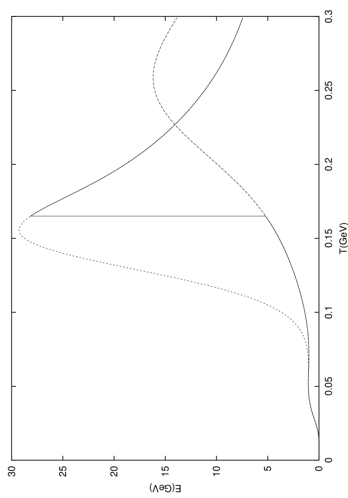
Figure 6: Heat capacity of the system. The solid line interpolates between the case with confinement below $T_{c}$ to the case without it above $T_{c}$ ($\mu_{B}$=$\mu_{s}$=0). The dotted and dashed line correspond respectively to the cases where color is allowed and without color.

The model can first be tested in the energy region below the transition temperature $T_{c}$, where the hadron gas should prevail. The confinement is effective and therefore we have to use the partition function $Z_{a=(0,0)}$ in the equations (7) and (8). We take, as an example, the measured total production rates of $\pi^{+}$ at 10 GeV/A, as reported in the SIS-GSI experiment [20]. The system considered was Au+Au and we assume that all particle participate, i.e. $N_{part}$=394. In Figure 2.3 of Ref. [20] a temperature of about $T=0.13$ GeV is reported. Assuming local strangeness conservation , $<s>=0$, we obtain a relation of $\mu_{s}$ versus $T$, which is depicted in Figure 7. From there we obtain, for the reported temperature, $\mu_{s}\approx 0.128$ GeV and via Figure 4 a value $\mu_{B}\approx 0.55$ GeV. In Figure 8 we show for a fixed value of $\mu_{B}$, physically acceptable at temperatures near $T=0.13$ GeV, the resulting total production rate of $\pi^{+}$ ($N_{\pi}$) as a function in the temperature $T$. For $T$ = 0.13 GeV the production rate is approximately 180 pions $\pi^{+}$, which is close to the value 160, which we have obtained by using Figure 2.3 of Ref. [20]. The good qualitative agreement with the experiment demonstrates that the present model is able, indeed, to describe, approximately, observed QCD features.

Figure 7: The dependence of $\mu_{s}$ on the temperature T, for $\mu_{B}=0.55$ GeV and assuming $<s>$=0, for the SIS-GSI experiment [20], Au+Au at 10 GeV/A.

Figure 8: Total production rate of $\pi^{+}$ for Au+Au at 10 GeV/A [20]. For $T=0.13$ GeV the total $\pi^{+}$ production rate is approximately 180. The value $\mu_{B}=0.55$ GeV was used in the calculations, as discussed in the text.

We have also determined ratios of particle production and some absolute production rates. The particle production is calculated for temperatures just below $T_{c}$, where only color zero states are allowed. This implies that the partition function to use is $Z_{(0,0)}$. We then apply Eq. (8). Note that in the expression of the particle-production ratios the partition function cancels out and only the dependence on the mass of the particles and the chemical potential remains. Figure 9 shows results for some particle-production ratios for beam energies $\sqrt{s}=130$A GeV. The experimental values are taken from Ref. [21], based on the experiment described in Ref. [22] (see also [23]). For baryons, only the ratios of particle and anti-particle production are shown because these expressions are independent of the mass of the baryon. As noted in (I) the masses of the baryons are not well reproduced because they are considered as consisting of three idealized fermions on top of the meson sea. The interaction to the meson sea is not taken into account yet, but indications about how to do it are given in (I).

Figure 9: Some particle production ratios for the beam energies $\sqrt{s}=130$ A GeV taken from Ref. [21]. The calculated values are shown with full squares and the experimental values are shown within error bars.

The central value of the $K^{-}/K^{+}$ production ratio, shown in Figure 9, was reproduced with the values $\mu_{s}=0.012$ GeV and $\mu_{B}=0.044$ GeV. The other ratios are predicted by the model. Considering the simplicity of the model, the ratios are found to be in a reasonable agreement with data.

In order to obtain the total yields for kaons and for the $\pi^{+}$ pions it is necessary to introduce further assumptions about the size of the QGP. The baryon density is given by $\frac{<B>}{V_{el}}$, where $V_{el}$ is the size of the representative volume, as explained before. In order to conserve, on the average, the baryon number we multiply the baryon density by the total volume and require that it must be equal to the total baryon number, given by the number of participants $N_{part}$. This leads to the total volume

$$V_{tot}=\frac{N_{part}V_{el}}{<B>_{a}}~{}~{}~{},$$ (9)

where the index $a$ refers to, as in the partition function, color ($a=c$) when the average value is calculated in the QGP and $a=(0,0)$ when it is calculated in the hadron gas. In the QGP the average value $<B>_{c}$ before the transition is smaller than the average value $<B>_{(0,0)}$ in the hadron gas after the transition. This is due to the small value of $Z_{(0,0)}$ at $T_{c}$, since many other possible color states are excluded from it which do contribute to $Z_{c}$. As a consequence, for $T=T_{c}$ the volume of the QGP phase, as a function of $N_{part}$, is much smaller than the one in the hadron gas phase. Assuming a sphere, the radius of the QGP phase is about 8 fm, and it changes to about 20 fm after the transition. This implies volumes of the order of approximately 2 $10^{3}$ fm³ and 3.4 $10^{4}$ fm³, respectively.

This transition is, as pointed out earlier, assumed to take place suddenly at $T_{c}$ (probably it should be smeared out but we cannot describe it with the present model). This implies that within the scenario assumed there is a rapid expansion of the volume caused by the transition from the QGP to the hadron phase, which should be observed as a large outward motion. One possible interpretation is that most of the pions are produced during the transition, liberating energy and provoking a rapid expansion of the system. The energy gained is represented by the jump between the lower and upper curves of Figure 5, but its origin cannot be explained by the present model, where confinement was shifted by hand.

Figure 10 shows the total pion yield as a function of the temperature $T$, corresponding to the Au+Au collision. The upper curve describes the total yield when all nucleons participate, while for the lower one we have taken $N_{part}=250$. This value agrees better with the experiment, as seen from the results, and it means that in the collision about 250 nucleons participate in the QGP. In Figure 11 the total kaon production rate is displayed. The upper curve corresponds to $K^{+}$ and the lower one to $K^{-}$ absolute production rates, respectively. In both cases $N_{part}=250$ was used, the same value used previously in the calculation of the pion yield. The ratio of the curves was already adjusted at the point corresponding to the $K^{+}/K^{-}$ ratio. The absolute production rate and the shape of the curve, however, is a prediction of the model (as far as we can talk about ”predictions” within this toy model). Considering the simplicity of the model it is surprising that the absolute production rate is well reproduced. This feature is common to other thermodynamical descriptions of the transition from the QGP to the hadron-gas [23, 21].

Figure 10: Total production rate of $\pi^{+}$. The upper curve is for $N_{part}=394$ (Au+Au) and the lower one is for $N_{part}=250$. Data are taken from [24]. Because of $\mu_{I}=0$, the production rate for $\pi^{-}$ coincides with the production rate for $\pi^{+}$.

Figure 11: Total production rate of $K^{+}$ (upper curve) and $K^{-}$ (lower curve) for $N_{part}=250$. Data are taken from [24].

Finally, in Figure 12, we show the calculated expectation values of the number of quark and gluon pairs as a function of the temperature T. At $T=0$ GeV the results correspond to the fractions of gluon pairs and fermion (quark-antiquark) pairs in the physical vacuum state. At high temperatures the gluon part increases and takes over the fermion part, which shows saturation. However, at the temperatures of interest, i.e. around the point of the phase transition $T_{c}\approx 0.16$ GeV, the gluon number is still suppressed with respect to the fermion pair number. This might be in favor of the ALCOR model [25] which supposes a suppression of gluons in the QGP and takes only constituent quarks and antiquarks into account. Note, that at $T=0.170$ GeV still a sensible amount of gluon pairs are present.

Figure 12: Expectation value of the fermion (quark-antiquark) and gluon pairs. The symbols $Z_{tot}$ and $Z_{00}$, on each curve, indicate if color was allowed. The upper indices $f$ and $g$ on the $Z$ refer to fermion and gluon pairs respectively.

5 Conclusions

We have presented a toy model of QCD. The model is described in (I) and in this paper we have focused on the thermodynamic properties, at equilibrium, emerging from the model. We have calculated the partition function with and without color, and studied the temperature dependence of some observables, like the internal energy, the heat capacity, and the production rates of particles. The parameters of the model were determined in (I), adjusting the meson spectrum at low energy. Without further parameters the internal energy, the heat capacity and some particle ratios were determined, as explained in the text.

We have applied the model to the case of the Au+Au collision at 10 GeV/A [20] and shown that it can reproduce qualitatively the absolute production rate of $\pi^{+}$. At this energy the QGP has not yet formed and, therefore, the results show that the model can be applied to study schematically the thermodynamics of a hadron gas.

Next, we have applied the model to energies where one assumes that the QGP has been already formed. The absolute production rate of $\pi^{+}$ and kaons were calculated, just below the transition temperature, by taking the number of participant nucleons ($N_{part}$) as an input. The agreement between calculated and experimental values was found to be satisfactory. Also, the resulting production rate was described reasonable well, once the $\mu_{s}$ chemical potential was fixed to yield the correct (observed central value) $\frac{K^{+}}{K^{-}}$ ratio. Some mass-independent baryon-antibaryon ratios, were qualitatively reproduced by the model predictions.

This demonstrates that the model is able to describe the general trend of QCD, in the finite temperature domain, and the transition to and from the quark gluon plasma.

6 Acknowledgment

We acknowledge financial support through the CONACyT-CONICET agreement under the project name Algebraic Methods in Nuclear and Subnuclear Physics and from CONACyT project number 32729-E. (S.J.) acknowledges financial support from the Deutscher Akademischer Austauschdienst (DAAD) and SRE, (S.L) acknowledges financial support from DGEP-UNAM. Financial help from DGAPA, project number IN119002, is also acknowledged.

References

- [1] S. Lerma, S. Jesgarz, P. O. Hess, O. Civitarese and M. Reboiro, Phys. Rev. C, (2003), this issue.
- [2] H. J. Lipkin, N. Meschkov and S. Glick, Nucl. Phys. A 62 (1965), 118.
- [3] D. Schütte and J. Da Providencia, Nucl. Phys. A 282(1977), 518.
- [4] S. Pittel, J. M. Arias, J. Dukelsky and A. Frank, Phys. Rev. C 50 (1994), 423.
- [5] J. Dobes and S. Pittel, Phys. Rev. C 57 (1998), 688
-
[6]
J. G. Hirsch, P. O. Hess and O. Civitarese,
Phys. Lett. B 390 (1997), 36;
O. Civitarese, P. O. Hess and J. G. Hirsch, Phys. Lett. B 412 (1997), 1;
J. G. Hirsch, P. O. Hess and O. Civitarese, Phys. Rev. C 56 (1997), 199 - [7] P. O. Hess, S. Lerma, J. C. López, C. R. Stephens and A. Weber, Eur. Phys. Jour. C 9 (1999), 121.
- [8] S. Lerma, S. Jesgarz, P. O. Hess, O. Civitarese and M. Reboiro, Phys. Rev. C 66 (2002), 045207
-
[9]
A. P. Szczepaniak, E. S. Swanson, C.-R. Jia and
S. R. Cotanch, Phys. Rev. Lett. 76 (1996), 2011;
E. S. Swanson and A. P. Szczepaniak, Phys. Rev. D 56 (1997), 5692;
P. Page, E. S. Swanson and A. P. Szczepaniak, Phys. Rev. D 59 (1999), 34016;
E. S. Swanson and A. P. Szczepaniak, Phys. Rev. D 59 (1999), 14035. - [10] U. Löring, B. Ch. Metsch and H. R. Petry, Eur. Phys. J. A 10 (2001), 309, 395 and 447.
-
[11]
B. Müller, The Physics of the Quark-Gluon
Plasma, Lecture Notes in Physics 225 (Springer, Heidelberg, 1985);
J. Lettessier and J. Rafleski, Hadrons and Quark-Gluon Plasma (Cambridge University Press, Cambridge, 2002). - [12] S. A. Bass, Pramana (2002), to be published, hetp: nucl-th/0202010 v2 and references therein.
-
[13]
J. P. Draayer and Y. Akiyama, Jour. Math. Phys.
14 (1973), 1904;
J. Escher and J. P. Draayer, J. Math. Phys. 39 (1998), 5123. - [14] M. Hamermesh, Group Theory and its Application to Physical Problems (Dover Publications, New York, 1989).
- [15] R. López, P. O. Hess, P. Rochford and J. P. Draayer, J. Phys. A 23 (1990), L229.
- [16] S. Lerma, program for the reduction of to , UNAM, Mexico (2002).
- [17] A. Klein and E. R. Marshalek, Rev. Mod. Phys. 63 (1991), 375.
- [18] K. T. Hecht, The Vector Coherent State Method and its Applications to Physical Problems of Higher Symmetries, Lecture Notes in Physics 290 (Springer-Verlag, Heidelberg, 1987).
- [19] W. Greiner, L. Neise and H. Stöcker, Thermodynamics and Statistical Mechanics, (Springer-Verlag, Heidelberg, 1994).
- [20] P. Senger and H. Ströbele, J. Phys. G 25 (1999) R59.
- [21] J. Rafelski and J. Letessier, nucl-th/0209084 (2002).
-
[22]
C. Adox, et al., PHENIX collaboration,
Phys. Rev. Lett. 89 (2002), 09-2302;
J. Castillo, et al., STAR collaboration, July 2002 Presentation at Nantes, Quark Matter 2002;
C. Adox, et al., PHENIX collaboration, Phys. Rev. Lett. 88 (2002), 24-2301;
C. Suir, et al., STAR collaboration, Phys. Rev. C 65 (2002), 04-1901;
C. Adler, STAR collaboration, Phys. Rev. C 65 (2002) 04-1901. -
[23]
P. Braun-Munzinger, I. Heppe and J. Stachel,
Phys. Lett. B 465 (1999), 15;
P. Braun-Munzinger and J. Stachel, J. Phys. G 28 (2002), 1971. - [24] The NA49 Collaboration, nucl-ex/0205002 (2002).
-
[25]
T. S. Biró, P. Lévai and J. Zimányi, Phys. Lett. B 347
(1995), 6;
T. S. Biró, P. Lévai and J. Zimányi, J. Phys. G 27 (2001), 439;
T. S. Biró, P. Lévai and J. Zimányi, J. Phys. G 28 (2002), 1561;