Scaling Distributions of Quarks, Mesons and Proton for all $p_{T}$, Energy and Centrality

Abstract

We present the evidences for the existence of a universal scaling behavior of the production of $\pi^{0}$ at all transverse momenta in heavy-ion collisions at all centralities and all collision energies. The corresponding scaling behavior of the quarks is then derived just before the quarks recombine with antiquarks to form the pions. The degradation effect of the dense medium on the quark $p_{T}$ is derived from the scaling distribution. In the recombination model it is then possible to calculate the $p_{T}$ distributions of the produced proton and kaon, which are scaling also. Experimentally verifiable predictions are made. Implications of the existence of the scaling behavior are discussed.

I Introduction

In two recent papers we have discussed the scaling properties of the large $p_{T}$ distributions of $\pi^{0}$ produced in Au+Au collisions at the relativistic heavy-ion collider (RHIC) and presented their implications. As reported in the first paper 1 , hereafter referred to as I, we found energy scaling at maximum centrality, while in the second paper 2 , referred to as II, we found centrality scaling at the highest energy. The two can be combined to yield one scaling distribution for all energy and centrality. In I we derive the quark distribution from the $\pi^{0}$ data in the framework of the recombination model; we now do the same for all centralities and determine the nature of degradation of the quark momentum in the dense medium, as we have done for the $\pi^{0}$ momentum in II. From the quark distribution we can calculate the proton distribution for all centralities. Moreover, we can extend our consideration to the production of kaons so that we can calculate not only the $p/\pi$ ratio, but also the $K/\pi$ ratio.

We are able to do all that for two essential reasons. The first is that the discovery of the scaling properties facilitates the analysis by avoiding the need to consider the variation of physics issues at different centralities and energies. The other is that the quark distribution we derive is for $q$ and $\bar{q}$ just before hadronization. It is not the result of some dynamical evolution starting from hard collisions, for which many complex issues must be considered 3 ; 4 ; 5 . The recombination model that we use can only address the hadronization problem of the soft partons at low virtuality, but at any $p_{T}$. From the pion data we infer the distributions of the soft $q$ and $\bar{q}$, which in turn are used to give the proton and kaon distributions through recombination. How the soft partons get to be where they are in the $p_{T}$ space is not considered. However, by studying the momentum degradation of the quarks, we gain from the centrality dependence of the $p_{T}$ distributions some understanding about how quarks lose momenta as they propagate through the dense medium. Experimentally verifiable predictions are made on the proton and kaon transverse momentum distributions.

The physical interpretation of the scaling variable is given at the very end, where the term transversity is suggested to refer to the difficulty of acquiring transverse motion. The broader implication on the creation of quark-gluon plasma is finally addressed.

II Scaling Distribution of Pions

From the preliminary PHENIX data of $\pi^{0}$ production in Au+Au collisions at RHIC 6 we have found a scaling distribution at midrapidity

$$\Phi(z)=A(N)K^{2}(s,N){1\over 2\pi p_{T}}{d^{2}N_{\pi}\over d\eta dp_{T}}\ ,$$ (1)

where

$$z=p_{T}/K(s,N)\ .$$ (2)

The symbol $N$ denotes the number of participants, $N_{\rm part}$, for brevity. The scaling factor $K(s,N)$ is first found in I for $N$ fixed at its maximum, $N_{\rm max}=350$, to be (in GeV/c)

$$K(s)=0.69+1.55\times 10^{-3}\sqrt{s}\ ,$$ (3)

where $\sqrt{s}$ is in units of GeV, and $K(s)$ is normalized to 1 at $\sqrt{s}=200$ GeV. When $N$ is allowed to vary, while $\sqrt{s}$ is fixed at 200 GeV, it is found in II that the scaling factor is

$$K(N)=1.226-6.36\times 10^{-4}N\ ,$$ (4)

normalized to 1 at $N=350$. We now combine the two and assume the factorizable form

$$K(s,N)=K(s)K(N)\ .$$ (5)

In this paper we investigate the centrality dependence mostly at $\sqrt{s}=200$ GeV. The normalization factor $A(N)$ in Eq. (1) is found in II to have a power-law dependence on the number of binary collisions, $N_{c}$,

$$A(N_{c})=530N_{c}^{-0.9}\ ,$$ (6)

where $N_{c}$ in turn depends on $N$ as

$$N_{c}=0.44N^{1.33}\ ,$$ (7)

a relationship that is determined from the tables listed in Refs. 7 ; 8 .

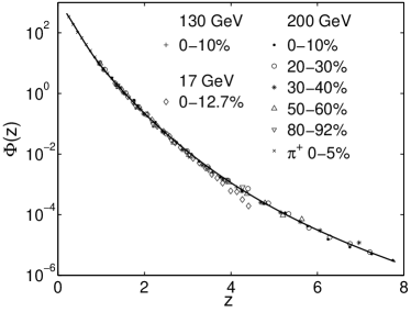
Figure 1: Scaling distribution of pion production. Data at $\sqrt{s}=130$ and 200 GeV are preliminary and were presented by PHENIX 6 ; 9 for Au+Au collisions. The data at 17 GeV are from WA98 8.1 for Pb+Pb collisions. The solid line is a fit by Eq. (8).

In Fig. 1 we show the combined plot of $\Phi(z)$ exhibiting the $\sqrt{s}=200$ GeV PHENIX data for 5 bins of centrality as well as the $\sqrt{s}=130$ GeV data at 0-10% centrality 6 and the 17 GeV data at 0-12.7% 8.1 . The $\pi^{0}$ data, which are only for $p_{T}>1$ GeV/c, are supplemented by the $\pi^{+}$ data for $p_{T}<1$ GeV/c at $\sqrt{s}=200$ GeV and 0-5% centrality 9 . Evidently, all the data points fall on one universal scaling distribution that is invariant under changes in $N$ and $\sqrt{s}$. The 17 GeV data are obtained by the WA98 Collaboration 8.1 for Pb+Pb collisions and show a slight departure from the universal curve for $z>3$. It should be recognized that those data points that deviate from the scaling distribution correspond to $p_{T}>3$ GeV/c, which is a $p_{T}$ range that represents a very large fraction of the total available energy of 17 GeV. Thus the kinematic constraint of energy conservation introduces a non-dynamical factor that suppresses the high-$p_{T}$ behavior, not present in the other data at $\sqrt{s}\geq$130 GeV. Such a violation of scaling is expected, and should not be regarded as an invalidation of the general scaling behavior we observe. On the contrary, it is amazing that the scaling behavior can cover such a wide range of $\sqrt{s}$, when most of the 17 GeV data points with $p_{T}<3$ GeV/c are included.

The scaling data points can be well fitted by 2

$$\Phi(z)=1200\,(z^{2}+2)^{-4.8}\left(1+25\,{\rm e}^{-4.5z}\right)\ ,$$ (8)

which is shown by the solid line in Fig. 1. This formula differs from the one given in I mainly by the addition of the exponential term, which reflects the statistical behavior at small $z$ represented by the $\pi^{+}$ data, but is insignificant at large $z$, where the power-law behavior is indicative of the effects of hard collisions.

A number of consequences of the scaling distribution, Eq. (8), can be examined directly. First, the integral

$${\cal I}=\int_{0}^{\infty}dzz\Phi(z)={A(N)\over 2\pi}{dN_{\pi^{0}}\over d\eta}$$ (9)

can be evaluated to yield ${\cal I}=46.2$. Using Eqs. (6) and (7) for $A(N)=A(N_{c}(N))$, we can calculate the $N$ dependence of $dN_{\pi^{0}}/d\eta$ at midrapidity. The data that are available for comparison are $dN_{\rm ch}/d\eta/(0.5N)$ vs $N$ at $\sqrt{s}=130$ GeV 8 , shown in Fig. 2. We plot in that figure in solid line our calculated result for $dN_{\pi^{\pm}}/d\eta/(0.5N)$, which is obtained from Eq. (9) by identifying $dN_{\pi^{\pm}}/d\eta$ with $2dN_{\pi^{0}}/d\eta$. Since $\pi^{\pm}$ is the dominant part of all charged particles, one should regard the comparison between the calculated $N_{\pi^{\pm}}$ and the measured $N_{\rm ch}$ to be satisfactory. Recall that although the $p/\pi$ ratio can exceed 1 around $p_{T}\approx 3$ GeV/c, it is small at small $p_{T}$ where the distributions are dominant, so the production of proton does not contribute to the integrated result as a large fraction of the total $dN_{\rm ch}/d\eta$.

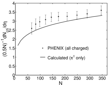
Figure 2: Calculated $dN_{\pi^{\pm}}/d\eta/(0.5N)$ compared to the data on $dN_{\rm ch}/d\eta/(0.5N)$ 8 .

Another consequence of $\Phi(z)$ is the possibility to calculate the nuclear modification factor

$$R_{AA}(p_{T})={d^{2}N_{\pi^{0}}^{AA}/d\eta dp_{T}\over N_{c}\,d^{2}N_{\pi^{0}}^{pp}/d\eta dp_{T}}\ .$$ (10)

The data available for that are given in Ref. 6 . We show in Fig. 3 the data for two centrality bins: 0-10% and 70-80%. The corresponding values of $N$ are 317 and 9.5, respectively 7 , for which the calculated $R_{AA}(p_{T})$ are shown by the solid and dash-dot lines. For $N_{\pi^{0}}^{pp}$ in the denominator of Eq. (10) we have used $N=2$. Experimentally, it is known that the peripheral nuclear collisions cannot be identified with $pp$ collisions. The ratio $R_{AA}(p_{T})$ is defined with $N_{\pi^{0}}^{pp}$ in the denominator so as to have a definitive experimental normalization. We calculate the ratio with $N=2$ in the denominator so that no additional experimental input is used. Our point is to show the consistency of $\Phi(z)$ when the value of $N$ is extrapolated to extreme limits. Toward that end we find the comparison between the data points and the calculated curves in Fig. 3 to be acceptable.

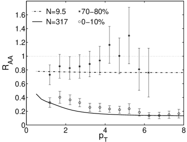
Figure 3: Nuclear modification factor $R_{AA}(p_{T})$ for $\pi^{0}$ production. The preliminary data are from PHENIX 6 . The lines are calculated results using $N=2$ extrapolation of $\Phi(z)$ for normalization rather than using independent $pp$ distribution.

The scaling distribution $\Phi(z)$ is a representation of the data over 9 orders of magnitude for all centralities and for all energies where data exist. Since the fit is done in the log scale in Fig. 1, one can expect some deviations in the linear scale, as the tests in Figs. 2 and 3 are done. The data must, of course, be self-consistent, so any discrepencies in those figures are due to the extrapolation of $\Phi(z)$ to very small $z$ in the calculation of $dN_{\pi^{0}}/d\eta$ and to very small $N$ for $R_{AA}$. We conclude from those tests that the formula (8) for $\Phi(z)$ is quite reliable even down to very small values of $z$ and $N$.

III Scaling Distribution of Quarks

From the scaling distribution of $\pi^{0}$ it is possible to derive the quark distribution in the framework of the recombination model. Those quarks have low virtuality (hence, soft) and are at the last stage of their existence just before hadronization. They are not to be confused with the partons at high virtuality (hence, hard) just after hard collisions. The evolution from the hard partons to the soft quarks through gluon radiation and conversion to quark pairs in the dense medium involve both perturbative and non-perturbative QCD processes that are complicated, only some of which can be calculated 3 ; 5 ; 10 ; 11 . The last step to hadrons is circumvented by use of the phenomenological fragmentation function that connects hard partons to hadrons directly. Our use of the recombination model treats only the last step from soft quarks to hadrons, and can make no statement about the evolutionary process that begins from hard collisions. What can be treated is how the soft quarks recombine in different combinations to form different hadrons. That is what we shall do in the following sections. Here we first derive the quark distributions and examine how they depend on centrality.

The application of the recombination model 12 ; 13 to the high $p_{T}$ problem has been discussed in I. The recombination of a $q$ and a $\bar{q}$ to form a $\pi^{0}$, where $q\bar{q}$ can be either $u\bar{u}$ or $d\bar{d}$, but not both $u\bar{u}$ and $d\bar{d}$, is described by [see I-Eq. (13)]

$${dN_{\pi^{0}}\over zdz}=\int dz_{1}dz_{2}\,z_{1}z_{2}F_{q\bar{q}}(z_{1},z_{2}){R}_{\pi}(z_{1},z_{2},z)\ ,$$ (11)

where our $dN_{\pi^{0}}/zdz$ is averaged over rapidity at midrapidity and over the azimuthal angle $\phi$ with the $1/2\pi$ factor included, unlike the experimental distribution $(2\pi)^{-1}d^{2}N_{\pi^{0}}/d\eta p_{T}dp_{T}$, which is an average over $\phi$ that shows the $1/2\pi$ factor explicitly, as in Eq. (1). The joint distribution $F_{q\bar{q}}(z_{1},z_{2})$ is assumed, for heavy-ion collisions, to have the factorizable form $F_{q\bar{q}}(z_{1},z_{2})=F_{q}(z_{1})F_{\bar{q}}(z_{2})$ with $F_{q}(z_{1})$ being the quark distribution in the scaling variable $z_{1}$, and $F_{\bar{q}}(z_{2})$ for the antiquark. The recombination function $R_{\pi}(z_{1},z_{2},z)$ depends on the wave function of the constituent quarks in the pion; in the valon model 1 ; 13 it is

$${R}_{\pi}(z_{1},z_{2},z)=z^{-2}\,\delta\left({z_{1}\over z}+{z_{2}\over z}-1\right)\ ,$$ (12)

where the valon distribution in the pion is determined by use of the data on Drell-Yan production by pion, which is the only way to probe the pion structure.

At $N=N_{\rm max}$, considered in I, the LHS of Eq. (11) is identified with $\Phi(z)$, which in I is scaling in $s$. Now for all centrality the LHS of Eq. (11) is replaced by the new $\Phi(z)$ given in Eq. (8), scaling in both $N$ and $s$, and on the RHS the new scaling $F_{q}(z_{1})$ and $F_{\bar{q}}(z_{2})$ are to be determined. Thus putting the various pieces together, we have

$$\Phi(z)=\int_{0}^{z}dz_{1}z_{1}\left(1-\frac{z_{1}}{z}\right)F_{q}(z_{1})F_{\bar{q}}(z-z_{1})\ .$$ (13)

There is no explicit dependence on $N$ or $s$ in this equation, but the $q$ and $\bar{q}$ distributions, being scale invariant, have implicit dependences on $p_{T}$ and $N$ that will be examined below.

Since the $q$ and $\bar{q}$ in Eq. (13) are at the end of their evolutionary processes, and are therefore soft partons dominated by the products of gluon conversion, their distributions can differ in normalization, but not significantly in their $z_{1}$ and $z_{2}$ dependences, a property that is supported by the observation that the $\bar{p}/p$ ratio is nearly constant in $p_{T}$ 14 . Denoting the $\bar{p}/p$ ratio by $c$, we thus use the relationship

$$F_{\bar{q}}(z)=c^{1/3}F_{q}(z)\ .$$ (14)

At RHIC energies $c$ is roughly 0.7; at SPS $c$ is about 0.13 14.1 ; 14.2 . Since $c$ depends on the energy $\sqrt{s}$, Eq. (14) is not strictly a scaling relationship. The smallness of $c$ at SPS energy is due to the difficulty of producing a large number of $\bar{p}$ compared to $p$ at $\sqrt{s}=17$ GeV 14.3 . Such a scaling violation is expected, just like the deviation of the diamond points at $z>3$ from the universal scaling curve in Fig. 1 for kinematical reasons. However, over the whole range of variation of $F_{q}(z)$ that we shall determine, the effect due to the variation of $c$ is small by comparison, as we shall see.

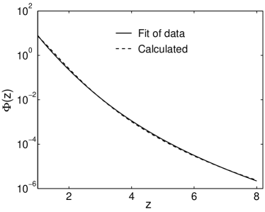
Figure 4: Comparison of fitted and calculated curves of $\Phi(z)$. The solid line is a plot of Eq. (8) obtained from the fit in Fig. 1. The dashed line is the result of the calculation using Eq. (13).

Let us put our emphasis on the scaling region of $c$ by setting $c=0.7$. Using that in Eq. (14) and then on the RHS of (13), with Eq. (8) on the LHS, we can vary the parametrization of $F_{q}(z)$ to achieve a good fit of $\Phi(z)$. Our result is

$$F_{q}(z)=15\,(z^{2}+0.47z+0.72)^{-4.25}\ .$$ (15)

In Fig. 4 we show a plot of Eq. (8) by the solid line and our fit of it using Eq. (15) in (13) by the dashed line. Clearly, the fit is very good. The quark distribution given by Eq. (15) is shown in Fig. 5 over a range of 9 orders of magnitude of variation. How would that be affected, if $c$ is lowered to 0.13? The normalization of $F_{q}(z)$ in Fig. 5 would be increased by a factor of $(0.7/0.13)^{1/6}=1.3$, which is insignificant compared to the 9 orders of magnitude of variation of $F_{q}(z)$.

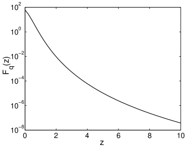
Figure 5: Scaling distribution of quarks before hadronization.

From Eq. (15) we can first determine the average $z$

$$\langle z\rangle={\int dzz^{2}F_{q}(z)\over\int dzzF_{q}(z)}=0.415.$$ (16)

We then define a new variable

$$u=z/\langle z\rangle\ ,$$ (17)

in terms of which we can define a new distribution

$$\psi_{q}(u) = F_{q}(z(u))\left/\int du\,uF_{q}(z(u))\right.$$

$$= \langle z\rangle^{2}F_{q}(z(u))\left/\int dz\,zF_{q}(z)\right.\ .$$

This distribution has not only the property that

$$\int du\ u\,\psi_{q}(u)=1$$ (19)

by definition, but also

$$\int du\ u^{2}\,\psi_{q}(u)=1\ .$$ (20)

These are the properties of a KNO-type distribution 15 . To be strictly KNO scaling, all higher moments should be independent of $N$, as we shall investigate. The virtue of the scaling variable $u$ is that it can be expressed directly in terms of $p_{T}$, since from Eqs. (2) and (17) we have

$$u=p_{T}/\langle p_{T}\rangle_{N}\ ,$$ (21)

where $\left<p_{T}\right>_{N}$ is the average $p_{T}$ at fixed centrality and $s$. Note that the scale factor $K(s,N)$ is common for the $p_{T}$ of both $\pi^{0}$ and $q$. In the case of pions 2 the variable $u$ can, in principle, be determined unambiguously from the experiments directly, unlike the variable $z$ that requires rescaling and fitting of the data at each $N$ and $s$. Indeed, the variable $u$ is constructed in the same spirit as in the original derivation of KNO scaling 15 . Although in the case of quarks here $u$ cannot be experimentally measured, it is useful to have a KNO distribution $\psi_{q}(u)$ as a goal for theoretical modeling, since the $u$ variable can more directly be related to the $p_{T}$ of the quarks.

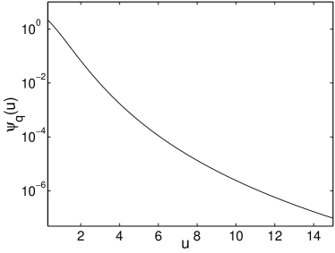
Figure 6: KNO-type distribution of quarks.

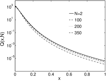
Figure 7: Centrality dependence of normalized quark distribution at $\sqrt{s}=200$ GeV.

From the definition in Eq. (18) we have

$$\psi_{q}(u)=1420\,(u^{2}+1.13u+4.18)^{-4.25}\ .$$ (22)

A plot of this distribution is shown in Fig. 6. The existence of such a scaling distribution in terms of an intuitive variable given in Eq. (21) suggests that there is a great deal of regularity in the interplay between $N$ and $p_{T}$. Remembering how $J/\psi$ production is expected to have an anomalous $p_{T}$ dependence in $AA$ collisions when deconfinement occurs 16 , we find the lack of irregularity in the $p_{T}$ distribution of the quarks to suggest that the subject of $p_{T}$ dependences of low-mass particles is not a fertile ground to find signals of quark-gluon plasma — unless, of course, scaling violation is dramatically found at LHC, say.

Having analytic forms for $F_{q}(z)$ and $\psi_{q}(u)$ enables us to investigate the degradation of the parton $p_{T}$ in the dense medium. To that end we define the momentum fraction variable

$$x=p_{T}/K_{0}\ ,$$ (23)

where $K_{0}$ is a fixed scale, which we take to be 10 Gev/c. It is tacitly assumed that there is no physics of interest here for $p_{T}>10$ GeV/c. If that is not the case, an upward revision of $K_{0}$ is trivial. From Eqs. (2) and (23) we have

$$z=x\,K_{0}/K(s,N)\ ,$$ (24)

and we may rewrite the scaling quark distribution as

$$F_{q}(z)=F_{q}(x,N)\ ,$$ (25)

where the $s$ dependence is suppressed. We can then define the normalized quark distribution

$$Q(x,N)=F_{q}(x,N)\left/\int_{0}^{1}dx\,xF_{q}(x,N)\right.\ .$$ (26)

The $x$ dependences of $Q(x,N)$ for various representative values of $N$ are shown in Fig. 7 for $\sqrt{s}=200$ GeV. It is evident that, as $N$ increases, the high $x$ tail of $Q(x,N)$ is suppressed, with a concurrent slight increase at very small $x$, since the integral of $Q(x,N)$ over $xdx$ is constant at 1. The crossover is at $x\approx 0.04$, corresponding to $p_{T}\approx 0.4$ Gev/c. Thus the effect of the dense medium is to degrade the $p_{T}$ of the quarks, which is a well known property, but in a very regular way that we now describe.

Let us define the ratio

$$R(x,N)={Q(x,N)\over Q(x,2)}$$ (27)

so that the suppression at most $x$ and enhancement at small $x$ can be exhibited more clearly, as shown in Fig. 8 for $\sqrt{s}=200$ GeV. Note that for $x>0.3$ the suppression is rather uniform. The rapid change in the range $0<x<0.3$ can be seen in a different plot, shown in Fig. 9. The decrease for $x>0.04$, as $N$ is increased, is now clear, as is the increase for $x<0.04$. It should be recognized that in normalizing $Q(x,N)$ by $Q(x,2)$ in Eq. (27) it is not important whether $Q(x,2)$ agrees well with the corresponding distribution in $pp$ collisions. The ratio removes the exponential dependence at small $x$ that is common for all $N$ and displays better the relative change as $N$ is varied. Also, the extrapolation to very small $x$ may not be accurate. The line for $x=0.01$ in Fig. 9 is intended mainly to give a rough idea of the nature of increase for $x<0.04$.

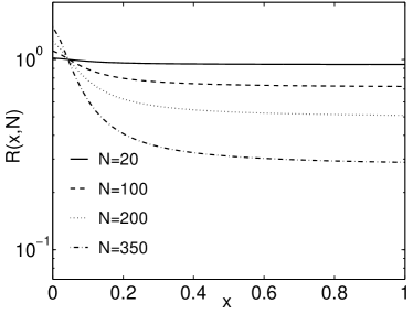
Figure 8: Ratio of quark distribution relative to $N=2$, exhibiting the degradation at $x>0.04$ and the enhancement at $x<0.04$ for $\sqrt{s}=200$ GeV.

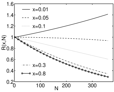
Figure 9: Same as Fig. 8 but plotted for various fixed values of $x$.

To quantify the degree of degradation, we take the moments of $Q(x,N)$ and define

$$Q_{n}(N)=\int_{0}^{1}dx\,x^{n+1}Q(x,N)\ .$$ (28)

We do not consider the order of the moment $n>5$, since higher moments demand more accuracy at higher $x$, which we cut off at $x=1$. The extrapolation of our scaling distribution $F_{q}(z)$ to higher $z$ is not without uncertainties. However, for $n\leq 5$ our analysis is reliable, and provides adequate insight into the nature of the degradation in the $0<x<1$ region. In Fig. 10 we show ln $Q_{n}(N)$ vs $N$ for $n=1,\cdots,5$; the relationship can be well approximated by linear dependence

$$\ln Q_{n}(N)=a_{n}-b_{n}N\ ,$$ (29)

where the slope $b_{n}$ is shown in the inset. Clearly, $b_{n}$ depends linearly on $n$

$$b_{n}=\lambda\,n\ ,\quad\quad\lambda=5.35\times 10^{-4}\ .$$ (30)

We can combine these two equations to write

$${d\over dN}\ln Q_{n}(N)=-\lambda\,n\ ,\qquad n\leq 5,$$ (31)

or

$$Q_{n}(N)=Q_{n}(N_{0})\,{\rm e}^{-\lambda\,n(N-N_{0})}\ .$$ (32)

Since Eq. (28) implies $Q_{n}(N)=\left<x^{n}\right>_{N}$, Eq. (32) is therefore also

$$\langle x^{n}\rangle_{N}=\langle x^{n}\rangle_{N_{0}}\,{\rm e}^{-\lambda\,n(N-N_{0})}\ .$$ (33)

In particular, for $n=1,N_{0}=2$, and $N=350$, we have

$$\langle x\rangle_{350}/\langle x\rangle_{2}=0.83\ .$$ (34)

Thus even at the maximum separation between $N$ and $N_{0}$, the average $p_{T}$ of the quarks loses only 17%. This is because even severe suppression of high-$x$ quarks cannot change significantly the average $\left<x\right>$, which is dominated by the low-$x$ behavior. However, the same cannot be said about the higher moments.

What we have found above are properties of the quarks before hadronization. Unfortunately, they cannot be checked directly by experiments. For testable predictions we now go to the study of proton and kaon formation, whose spectra can be measured experimentally.

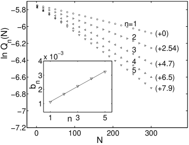
Figure 10: Centrality dependence of the moments, $Q_{n}(N)$, whose log values are raised by the quantities in the parentheses. The inset shows the slopes $b_{n}$, the line being a linear fit.

IV Scaling Distribution of Proton

The quarks considered in the preceding section can not only combine with antiquarks to form pions, but also combine with other quarks to form protons. The formulation of the problem is discussed in I, where centrality variation is not considered. Now we allow $N$ to vary, starting from the new quark distribution $F_{q}(z)$, whose scaling behavior includes the implicit dependence on centrality. As before, the treatment of proton production is not reliable at low $z$, where $p_{T}$ of the proton is low enough to make the mass effect important. Our calculation that is scale invariant cannot take into account the mass-dependent effects.

The proton distribution arising from the recombination of $uud$ quarks is given by 1

$${dN_{p}\over zdz}=\int dz_{1}dz_{2}dz_{3}\,z_{1}z_{2}z_{3}F_{uud}(z_{1},z_{2},z_{3}){R}_{p}(z_{1},z_{2},z_{3},z)\ ,$$ (35)

where

$$F_{uud}(z_{1},z_{2},z_{3})=F_{u}(z_{1})F_{u}(z_{2})F_{d}(z_{3})\ ,$$ (36)

and

$${R}_{p}(z_{1},z_{2},z_{3},z)=0.057\,z^{-2}G_{p}(\xi_{1},\xi_{2},\xi_{3})\ .$$ (37)

$G_{p}(\xi_{1},\xi_{2},\xi_{3})$ is the valon distribution in a proton, expressed in terms of the valon momentum fractions $\xi_{i}=z_{i}/z$ 17 . It is determined from the parton distributions that fit the deep inelastic scattering data, and is

$$G_{p}(\xi_{1},\xi_{2},\xi_{3})=g\,(\xi_{1}\xi_{2})^{\alpha}\,\xi_{3}^{\beta}\,\delta(\xi_{1}+\xi_{2}+\xi_{3}-1)\ ,$$ (38)

where

$$\alpha=1.755,\qquad\qquad\beta=1.05\ ,$$ (39)

$$g=[B(\alpha+1,\beta+1)B(\alpha+1,\alpha+\beta+2)]^{-1}\ .$$ (40)

The recombination function for the proton is more complicated than that for the pion because the proton is not as tightly bound as the pion in terms of the constituent quarks masses, but the procedures for the determination of the recombination functions are similar.

Equation (35) is derived in I for $N=N_{\rm max}$. For $N<N_{\rm max}$ the new scaling function for $F_{q}$ in Eq. (15) is to be used for the quark distributions $F_{u}$ and $F_{d}$ in Eq. (36). The resulting integral is to be identified with the new proton scaling distribution $\Phi_{p}(z)$, as in the pion case. We show in Fig. 11 the result on $\Phi_{p}(z)$, for which only the $z>3$ part is plotted, since it is unreliable for $z<3$ due to the neglect of the mass effect.

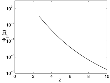
Figure 11: Scaling distribution for proton.

The relationship between the calculated $\Phi_{p}(z)$ and the $p_{T}$ distribution $dN_{p}/p_{T}dp_{T}(s,N)$ is

$$\Phi_{p}(z)=A_{p}(N)K^{2}_{p}(s,N){dN_{p}\over p_{T}dp_{T}}(s,N)\ ,$$ (41)

where, we repeat, our $dN_{p}/p_{T}dp_{T}$ corresponds to the experimental $(2\pi p_{T})^{-1}d^{2}N_{p}/d\eta dp_{T}$ [cf. Eq. (1)]. We have added a subscript $p$ to each function in Eq. (41) to emphasize their reference to proton; indeed, we should similarly add a subscript $\pi$ to the corresponding functions in Eq. (1) to clarify their differences, as we shall do below when we compare $p$ and $\pi$ production. Whereas Eq. (1) is determined by the phenomenological analysis of the $\pi^{0}$ data in II, there are no similar data on the $p$ spectra to confirm Eq. (41). However, on theoretical grounds we expect that relationship to exist for the following reasons. First, since the quark distribution is scale invariant, the recombination model implies that there is a scaling distribution $\Phi_{p}(z)$ for the proton, as we have calculated. That gives the LHS of Eq. (41). On the RHS we expect $K_{p}(s,N)=K_{\pi}(s,N)=K_{q}(s,N)$, since the same scaling variable $z$ has been used for pion, quark and proton. Without that universal variable $z$ the recombination model cannot be formulated in the form of Eqs. (11) and (35). Finally, we conjecture that

$$A_{p}(N)=A_{\pi}^{3/2}(N)$$ (42)

on the grounds of internal consistency, since the comparison among Eqs. (1), (11) and (13) suggests that $F_{q}$ implicitly absorbs an $A_{\pi}^{1/2}$ factor. When that factor is applied to Eqs. (35), (36) and (41), we expect Eq. (42) to follow. This conjecture can be independently checked when the centrality dependence of the proton distribution at high $p_{T}$ becomes available and the existence of the scaling $\Phi_{p}(z)$ can then be examined directly from the data, as is done in II. If the conjecture is verified, then the data provide empirical evidence for proton being the hadronization product of three quarks, rather than other mechnisms such as gluon junction 4 ; 19 .

One way to check Eq. (42) is to calculate the $p/\pi$ ratio, $R_{p/\pi}$, at different centrality bins, where

$$R_{p/\pi}(p_{T},N)=\left.{dN_{p}\over p_{T}dp_{T}}(N)\right/{dN_{\pi}\over p_{T}dp_{T}}(N)\ .$$ (43)

In I this ratio has been calculated for $N=N_{\rm max}$. Using Eqs. (41) and (42) we now can calculate it for $N<N_{\rm max}$. There is no data in the $p_{T}$ range where our prediction is reliable. However, PHENIX does have preliminary data on $R_{p/\pi}$ for $p_{T}<3.7$ GeV/c for two centrality bins, 0-5% and 60-91% 14 . They differ by roughly a factor of 3 with large errors for $p_{T}\approx 3$ GeV/c. Assuming that the ratio of ratios is likely to remain the same at higher $p_{T}$, we can calculate it for comparison, with the definition

$$r(p_{T})=R_{p/\pi}(p_{T},N=350)/R_{p/\pi}(p_{T},N=15)\ ,$$ (44)

where $N=15$ is taken to correspond to 60-91% centrality. The result is shown in Fig. 12 for $\sqrt{s}=200$ GeV. While the tendency of $r(p_{T})$ to increase at low $p_{T}$ is disturbing, the level of $r(p_{T})\approx 3$ for $p_{T}>5$ GeV/c is in rough agreement with the data at $p_{T}\approx 3$ GeV/c. If $A_{p}(N)$ were the same as $A_{\pi}(N)$, then $r(p_{T})$ would be much lower by a factor of 8.4 and can be ruled out even by the preliminary data 14 . Thus, until sufficient data become available to test directly the scaling formula (41) for protons, we shall use Eq. (42) for the normalization factor.

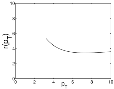
Figure 12: The ratio of the $p/\pi$ ratio at $N=350$ to the same at $N=15$ for $\sqrt{s}=200$ GeV.

On the basis of Eq. (41) we now can calculate the $p_{T}$ distributions, $dN_{p}/p_{T}dp_{T}$, that are experimentally measurable. They are shown in Fig. 13 for $N=30,150,$ and 350 for $\sqrt{s}=200$ GeV. It is interesting to note that the distributions for $N=150$ and 350 differ only slightly in the log scale, due undoubtedly to the near cancellation of the two opposing properties: the increase of the number of hard collisions at higher $N$ and the suppression of high $p_{T}$ protons in larger dense medium.

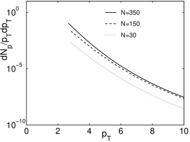
Figure 13: The $p_{T}$ distribution for proton at three values of $N$ for $\sqrt{s}=200$ GeV.

V Scaling Distribution of Kaons

For the production of kaons in the recombination model we need two inputs: the strange quark distribution and the recombination function for a $K$ meson. The former has been considered in our study of the strangeness enhancement problem in heavy-ion collisions 18 . The latter is given in Ref. 13 .

It is known that the number of $\Lambda$ and $\Sigma$ hyperons produced in heavy-ion collisions is enhanced by more than a factor of 2. Since the enhancement is due mainly to gluon conversion and Pauli blocking, the relevant question in the context of the parton model is what the percentage of the gluon conversion into the strange quarks is. The amazing answer found in Ref. 18 is that it is only 8%. Due to the large number of gluons produced in heavy-ion collisions that is enough to raise the strange quark density by a factor of 2.1 to 2.3 from the intrinsic level in a free proton, depending on collision energy.

To be precise, let us use the notation where the symbols $\ell$ and $s$ denote the total number of light and strange quarks, respectively, $\ell$ being $u+d$, in contrast to $q$ being $u$ or $d$. Let $\ell_{v},\ell_{s},s_{s}$ and $g$ denote the numbers of valence quarks, light sea quarks, strange quarks and gluons, respectively, before the gluons are converted to $\ell\bar{\ell}$ and $s\bar{s}$ for recombination to form hadrons. Since only the ratios of these numbers will be relevant below, they will be given modulo a common multiplicative factor that need not be specified. The numbers for RHIC at 130 GeV are 18

$$\ell_{v} = 0.30\ ,\quad\quad\ell_{s}=0.37\ ,$$ (45)

$$s_{s} = 0.18\ ,\quad\quad g=2.46\ .$$

It is also found that the fraction of gluon conversion to the strange sector is $\gamma=0.08$, i.e.,

$$s_{c}=\gamma g\ ,\quad\quad\ell_{c}=(1-\gamma)g\ ,$$ (46)

where the subscript $c$ denotes converted quarks. The net strange to light quark ratio after conversion is then

$${s\over\ell}={s_{s}+s_{c}\over\ell_{v}+\ell_{s}+\ell_{c}}=0.128\ .$$ (47)

Setting $u=d$ for simplicity, we have $\ell=2q$ and

$$s/q=0.256\ .$$ (48)

Since $s_{c}=\gamma g=0.197,$ the strange quark multiplicity originally at $s_{s}$ is more than doubled by gluon conversion.

The above consideration is at the quark level. How that translates to hadron abundance must take into account hyperon production in addition to kaon production, since the effects of associated production cannot be ignored. The problem of partitioning the total strange quark numbers into various channels of strange hadrons competing for those quarks has been treated in Ref. 18 . It is found there that the fraction $\kappa$ of $s$ quark forming $\bar{K}$ and $\bar{\kappa}$ of $\bar{s}$ antiquark forming $K$ can be deduced from the data. That is, defining

$$\bar{K}=\kappa s\ ,\quad\quad K=\bar{\kappa}\bar{s}\ ,$$ (49)

where $\bar{K}=K^{-}+\bar{K}^{0}$ and $K=K^{+}+K^{0}$ denote the numbers of $K$ mesons of various types, one has at 130 GeV collision energy

$$\kappa=0.628\ ,\quad\quad\bar{\kappa}=0.713\ .$$ (50)

For the purpose of calculating $K^{+}/\pi^{+}$ ratio, let us use $\bar{s}^{\prime}$ to denote the number of $\bar{s}$ quarks to recombine with $u$ quark to form $K^{+}$, and we have

$$\bar{s}^{\prime}={0.256\over 2}\bar{\kappa}q=0.091q\ .$$ (51)

We shall assume that the $z$ distribution of the $\bar{s}^{\prime}$ quark is the same, apart from normalization, as that of the $u$ quark, so we get

$$F_{\bar{s}^{\prime}}(z)=0.091F_{q}(z)\ .$$ (52)

In the recombination model we expect the produced $K^{+}$ to have also a scaling distribution

$$\Phi_{K}(z)=\int dz_{1}dz_{2}\,z_{1}z_{2}F_{q}(z_{1})F_{\bar{s}^{\prime}}(z_{2}){R}_{K}(z_{1},z_{2},z)\ .$$ (53)

The recombination function for the $K$ meson is similar to that of the pion given in I

$$R_{K}(z_{1},z_{2},z)=R_{K}^{0}\,z^{-2}\,G_{K}\left({z_{1}\over z},{z_{2}\over z}\right),$$ (54)

where $G_{K}(\xi_{1},\xi_{2})$ is the valon distribution in the $K$ meson 13

$$G_{K}(\xi_{1},\xi_{2})=g_{K}\,\xi_{1}^{a}\xi_{2}^{b}\,\delta(\xi_{1}+\xi_{2}-1)$$ (55)

with $g_{K}=B(a+1,b+1)^{-1}$. The parameters $a$ and $b$ are determined from the analysis of $Kp$ collisions and are found to be $a=1$ and $b=2$ (see the second paper in Ref. 13 ). Since $K^{+}$ is the only state in the pseudoscalar octet that has $u\bar{s}$ content, we have $R_{K}^{0}=1$ and thus

$$R_{K}(z_{1},z_{2},z)={1\over B(2,3)}{z_{1}z_{2}^{2}\over z^{5}}\,\delta\left({z_{1}\over z}+{z_{2}\over z}-1\right).$$ (56)

We now can calculate $\Phi_{K}(z)$ using Eqs. (15), (52), (53), and (56). Since for $\Phi_{K}(z)$ we have, as in Eq. (41),

$$\Phi_{K}(z)=A_{K}(N)K^{2}_{K}(s,N){dN_{K}\over p_{T}dp_{T}}(s,N)\ ,$$ (57)

where $A_{K}=A_{\pi}$ and $K_{K}=K_{\pi}$, we obtain for the $K^{+}/\pi^{+}$ ratio

$$R_{K/\pi}(p_{T},N)=\left.{dN_{K}\over p_{T}dp_{T}}\right/{dN_{\pi}\over p_{T}dp_{T}}={\Phi_{K}(z(p_{T},N))\over\Phi_{\pi}(z(p_{T},N))}\ ,$$ (58)

where $\pi^{+}$ is taken to be the same as $\pi^{0}$.

In Fig. 14 we show $R_{K/\pi}(p_{T})$ for $N=350$ and 200 and $\sqrt{s}=130$ GeV. Since the determination of $\kappa$ and $\bar{\kappa}$ in Eq. (50) is by use of the data on particle ratios, which are not reliable for non-central collisions, we have no confidence in the strangeness enhancement factor deduced when $N$ is low. For $N>200$ Fig. 14 shows that the $K/\pi$ ratio is not sensitive to centrality, and only mildly dependent on $p_{T}$. This result awaits direct check by experimental data.

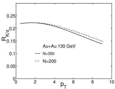
Figure 14: The $K/\pi$ ratio at two values of $N$ for $\sqrt{s}=130$ GeV.

VI Conclusion

From the scaling distribution $\Phi(z)$ obtained from the data on $\pi^{0}$ production, we have derived many quantities by use of the recombination model. They are the distributions of quarks, protons, and kaons, and their respective dependences on centrality. All that is made possible by the discovery of the universal function $\Phi(z)$ valid for all centrality and collision energy. The scaling variable $z$ that unites the $p_{T}$ dependences for all $N$ and $\sqrt{s}$ quantifies the difficulty of producing transverse motion, and for that interpretation it can be termed transversity. A particle produced at a particular $p_{T}$ at high $\sqrt{s}$ has a lower transversity than that of the same particle produced at the same $p_{T}$ but at a lower $\sqrt{s}$, because it is easier in the former case that involves a smaller momentum fraction. Similarly, it is easier to produce a particle at a given high $p_{T}$ when $N$ is low than to do the same at a higher $N$ because there is less degradation of the transverse momentum at lower $N$. Thus the former particle has lower transversity than the latter. With this way of viewing transverse motion we see that it is the transversity of the produced particles that has the universal property at whatever centrality and collision energy.

The quantitative results that we have obtained have their limitations due to the assumptions that we have made. For example, for the proton $z$ distribution we have assumed that $F_{\bar{q}}(z)/F_{q}(z)$ is a constant, which has some phenomenological support in that the observed $\bar{p}/p$ ratio is roughly constant in $p_{T}$; however, that ratio fails to maintain constancy at very peripheral collisions. Thus our result is not likely to be valid when $N$ is very low. Similarly, whether $F_{\bar{s}^{\prime}}(z)/F_{q}(z)$ is a constant and over what range of $N$, if it is, are not known. The centrality dependence of the strangeness fraction of gluon conversion is also unknown. Our result on $K/\pi$ ratio can therefore only be regarded as preliminary, pending experimental guidance to improve our simplifying assumptions. Despite these uncertainties for non-central collisions, the recombination model has enabled us to calculate the scaling behavior of the quark, proton, and kaon distributions, the latter two of which are subject to direct experimental test.

For non-central collisions we have only calculated the $p_{T}$ distribution, averaged over the azimuthal angle $\phi$. Clearly, the dependence on $\phi$ is important as it contains dynamical information. It will be very interesting to investigate whether centrality scaling persists in restricted $\phi$ bins, and if it does, how the scaling curves depend on $\phi$. On the basis of the universality in transversity distribution, we expect that such $\phi$-dependent scaling curves can be put into an overall $\phi$-independent scaling curve upon rescaling. At the price of lower statistics this can be checked by appropriate analysis of the $\pi^{0}$ production data.

Ultimately, the important issue to focus on is the implication of the existence of the scaling behavior on the possible formation of quark-gluon plasma. At this stage of our understanding a conservative statement that can be made is that the discovery of scaling violation might provide a strong hint for a drastic change of dynamics, possibly associated with a phase transition. Without waiting for LHC to enlighten us with that possibility, a more urgent issue to settle is why, if the quark-gluon plasma has been created already at existing collision energies, the change of the nature of the dense medium does not affect the scaling behavior that we have found to be universal between 17 and 200 GeV. Either the scaling behavior is insensitive to the change, or the change has already occurred at collision energy less than 17 GeV. If both of these alternatives are incorrect, then the only way out is that quark-gluon plasma has not yet been created at RHIC. These are the unintended, but remarkable, consequences of the scaling behavior. It is thus paramount to understand whether a phase transition can lead to a violation of the scaling behavior found here.

References

- (1) R.C. Hwa and C.B. Yang, nucl-th/0211010 (to be published in Phys. Rev. C), hereafter referred to as I.
- (2) R.C. Hwa and C.B. Yang, nucl-th/0301004, hereafter referred to as II.
- (3) X. N. Wang, Phys. Rev. C 58, 2321 (1998); ibid 61, 064910 (2000); ibid 63, 054902 (2002).
- (4) I. Vitev and M. Gyulassy, Phys. Rev. C 65, 041902 (2002).
- (5) For a recent review see R. Baier, hep-ph/0209038, talk given at Quark Matter 2002, Nantes, France (2002).
- (6) D. d’Enterria (PHENIX Collaboration), hep-ex/0209051, talk given at Quark Matter 2002, Nantes, France (2002).
- (7) D. Kharzeev and M. Nardi, Phys. Lett. B 507, 121 (2001).
- (8) K. Adcox et al. (PHENIX Collaboration) Phys. Rev. Lett. 86, 3500 (2001).
- (9) K. Reygers (WA98 and PHENIX Collaborations), nucl-ex/0202018.
- (10) T. Chujo (PHENIX Collaboration), nucl-ex/0209027, talk given at Quark Matter 2002, Nantes, France (2002).
- (11) X. N. Wang and M. Gyulassy, Phys. Rev. Lett. 68, 1480 (1992); E. Wang and X. N. Wang, ibid. 89, 162301 (2002).
- (12) R. Baier, Yu. L. Dokshitzer, A. H. Mueller, S. Peigné, and D. Schiff, Nucl. Phys. B484, 265 (1997); R. Baier, Yu. L. Dokshitzer, A. H. Mueller, and D. Schiff, Phys. Rev. C 58, 1706 (1998).
- (13) K. P. Das and R. C. Hwa, Phys. Lett. 68B, 459 (1977); R. C. Hwa, Phys. Rev. D22, 1593 (1980).
- (14) R. C. Hwa, and C. B. Yang, Phys. Rev. C 66, 025205 (2002); R. C. Hwa, and C. B. Yang, ibid. 65, 034905 (2002).
- (15) T. Sakaguchi (PHENIX Collaboration), nucl-ex/0209030, talk given at Quark Matter 2002, Nantes, France (2002).
- (16) F. Sikler et al (NA49 Collaboration) Nucl. Phys. A 661, 45c (1999).
- (17) C. Adler et al (STAR Collaboration) Nucl. Phys. A 698, 64c (2002).
- (18) H.Z. Huang, Nucl. Phys. A 698, 663c (2002).
- (19) Z. Koba, H. B. Nielsen, and P. Olesen, Nucl. Phys. B40, 317 (1972).
- (20) K. Karsch and R. Petronzio, Phys. Lett. B 37, 1851 (1988).
- (21) R. C. Hwa, and C. B. Yang, Phys. Rev. C 66, 025204 (2002).
- (22) D. Kharzeev, Phys. Lett. B 378, 238 (1996).
- (23) R. C. Hwa, and C. B. Yang, Phys. Rev. C 66, 064903 (2002).