The Density Matrix Renormalization Group in Nuclear Physics: A Status Report

Abstract

We report on the current status of recent efforts to develop the Density Matrix Renormalization Group method for use in large-scale nuclear shell-model calculations.

PACS numbers: 21.60.Cs, 05.10.Cc

I Introduction

The Density Matrix Renormalization Group or DMRG was originally introduced by Steven White in the early 1990s to treat the properties of quantum lattices[1]. It quickly proved to be enormously successful, producing for the ground state energy of the spin-1 Heisenberg chain results that were accurate to 12 significant figures, well beyond what was achievable with any other approximate many-body method. Subsequently, the method was applied with great success to other 1D lattices, including spin chains and t-J and Hubbard models[2]. The model in its original formalism, which worked in terms of real space lattice sites, has also been applied, though with much less success, to some 2D lattices as well.

Subsequently, the DMRG method was reformulated[3, 4] so as not to work solely in terms of real space lattice sites. In this extended version, the method has proven extremely useful in the description of finite Fermi systems, as arise for example in quantum chemistry[5] and in the physics of small metallic grains[6]. The successes achieved in these domains suggests the possible usefulness of the DMRG method in the description of another finite Fermi system, the atomic nucleus. In this paper, we briefly review the current status of our recent efforts to implement such a program[7, 8].

The outline of the presentation is as follows. In Section II, we briefly review the key elements of the DMRG method, whether for quantum lattices or finite fermi systems. In Section III, we describe our first efforts to apply a variant of the method to real nuclei. As we will see, the results are not particularly good. In Section IV, we describe a possible way to improve the DMRG methodology, to more appropriately tune it to the the physics of nuclei. Finally, in Section V, we summarize the key points of the presentation.

II Brief Review of the DMRG formalism

The DMRG is a method for systematically taking into account in an approximate fashion all the degrees of freedom of a problem, without letting the problem get numerically out of hand. The method is rooted in Ken Wilson’s “onion” picture[9], schematically illustrated in figure 1. Each layer of the onion should be thought of as another degree of freedom. It could be a site on a lattice or it could be a single-particle orbital in a problem involving a finite fermi system.

FIG. 1.: Schematic illustration of Wilson’s onion picture of the Renormalization Group. The solid lines refer to the layers already treated, i.e. comprising the block; the dashed line refers to the layer added to enlarge the block; the dotted lines refer to the layers still to be treated.

Assume that we have already taken into account a given number of layers of the onion (illustrated by solid lines in the figure) and that the total number of states we have kept to describe that portion of the system, which we call the block, is $p$. Assume furthermore that the next layer of the onion (illustrated by a dashed line) contains another $s$ states. If we add the new layer to the block, the total number of states in the enlarged block will be $p\times s$. The basic idea of all Renormalization Group Methods, whether Wilson’s numerical Renormalization Group (RG) or White’s DMRG, is to somehow truncate from these $p\times s$ states to the most important $p$ states, the same number we had before enlarging the block. We would then add the next layer of the onion, truncating afterwards to the most important $p$ states again. And we would do this until all layers have been treated. We would carry out the calculation as a function of $p$, stopping when the change with increasing $p$ is sufficiently small.

To this point, we have not yet said how to implement the truncation. Indeed, the answer is different in the usual Wilson RG method and in White’s DMRG method.

In Wilson’s method, one simply diagonalizes the hamiltonian in the enlarged block, including the extra layer, and then truncates to the lowest $p$ eigenstates.

In White’s DMRG method the idea is different, and better. Here, one considers the enlarged block in a medium that approximates the rest of the system. The entire system - enlarged block + medium - is referred to as the superblock. The hamiltonian is diagonalized in the superblock, yielding a ground state wave function

$$|\Psi>~{}=~{}\sum_{i=1,p\times s}\sum_{j=1,t}\Psi_{ij}|i>_{B}|j>_{M}$$ (1)

where $B$ denotes the states in the block, $M$ the states in the medium and $t$ the number of states in the medium.

The reduced density matrix for the enlarged block in the ground state,

$$\rho^{B}_{ii^{\prime}}=\sum_{j=1,t}\Psi_{ij}\Psi^{*}_{i^{\prime}j}~{},$$ (2)

is then constructed and diagonalized,

$$\rho^{B}|u^{\alpha}>_{B}~{}=~{}\omega^{B}_{\alpha}~{}|u^{\alpha}>_{B}~{}.$$ (3)

Those eigenstates $|u^{\alpha}>_{B}$ with the largest eigenvalues $\omega^{B}_{\alpha}$ are the most important states of the enlarged block in the ground state of the superblock, i.e. of the system. One thus truncates to the $p$ states of the enlarged block with the largest density matrix eigenvalues.

Details on how this can be efficiently done can be found in the Proceedings of this series of symposia in 2001 [8].

A The finite versus infinite algorithm

The method described above, where one passes through the set of onion layers a single time, is referred to as the infinite DMRG algorithm. Depending on the manner in which correlations between layers fall off, this method can sometimes lead to an accurate representation of the ground state of the system and perhaps some excited states as well . Usually, it does not, however, since the early layers know nothing of the physics of those treated subsequently. Thus the blocks are only being optimized with respect to the layers that make them up. This suggests the use of a “sweeping” algorithm, whereby once all layers have been sampled we reverse direction and update the blocks based on the information of the previous “sweep”. Such a sweeping algorithm can be iteratively implemented until acceptable convergence in the results has been achieved. The latter procedure, in which we sweep back and forth through the onion, is called the finite algorithm. This is the method usually needed when dealing with finite fermi systems, like nuclei.

B The p-h DMRG method

In the description of finite fermi systems, it is natural to use a basis of single-particle states and to implement the DMRG by iteratively adding their effects. An important feature of such systems is the presence of a fermi surface, which divides the set of single-particle levels into those that are primarily occupied and those that are primarily filled. It is possible to incorporate this into the DMRG algorithm in the following way.

FIG. 2.: Schematic illustration of the p-h DMRG method for finite fermi systems. The single-particle levels are divided into primarily occupied hole levels and primarily empty particle levels. The first two levels above the fermi energy $E_{F}$ have been formed into a particle block and the first two below the fermi energy have been formed into a hole block. The third levels above and below are then added to form enlarged blocks.

Consider the set of single-particle levels shown in figure 2. Note that they are divided into two sets. There are particle levels - those that are primarily empty - and hole levels - those that are primarily filled. In the p-h DMRG method, one starts with the levels nearest to the fermi surface, which make up particle and hole blocks, and then gradually adds to them levels further away. The figure is meant to signify that we have already created particle and hole blocks involving the first two available levels, respectively, and that we then enlarge them by adding the third level(s). The particle block then serves as the medium for the holes and the hole block as the medium for the particles as we implement the DMRG truncation strategy. This process is continued until all particle and all hole levels have been treated.

The p-h DMRG method is particularly useful when the infinite algorithm can be used. When it is necessary to introduce sweeping, it becomes too cumbersome to implement because of the preponderance of blocks that have to be considered. This is especially true for nuclei in which one has two kinds of particles and thus twice as many blocks. In such cases, there are four distinct blocks – proton particle, proton hole, neutron particle and neutron hole – and this makes it very hard to implement sweeping.

Nevertheless, the first calculations carried out for nuclei using the DMRG method were based on the p-h algorithm. The hope was that the correlations would fall off sufficiently rapidly as we progress away from the fermi surface, making the infinite algorithm acceptable. It is these results, the first that we have obtained using the DMRG for realistic nuclei, that will be presented in the next section.

III Application of the p-h DMRG method to ${}^{24}Mg$

As a first application of the p-h DMRG method in nuclear structure, we considered the nucleus ${}^{24}Mg$, with four neutrons and four protons outside doubly-magic ${}^{16}O$. As is usual in the shell model, we assumed that ${}^{16}O$ is inert and distributed the remaining 8 nucleons over the orbits of the $2s-1d$ shell only. This shell-model problem is small – perhaps too small – and can be solved trivially by exact shell-model diagonalization.

FIG. 3.: Schematic illustration of the splitting of the spherical single–particle levels of the $sd$–shell into a set of doubly–degenerate levels by an axially–deformed Hartree–Fock calculation. The dashed line represents the Fermi energy ($E_{F}$), which separates the particle levels from the hole levels. Each doubly–degenerate level is labelled by its angular momentum projection on the intrinsic z-axis.

The results we show were obtained using a Hartree Fock single-particle basis to define the single-particle levels and their order. These levels are illustrated in figure 3.

There is a great calculational simplification when one uses a single-particle basis in which all levels are essentially the same. And indeed when one uses an axially deformed HF basis, all levels are doubly degenerate and thus very similar in structure.

The calculations were done using the usual USD effective hamiltonian for the $2s-1d$ shell.

In figure 4, we show results for the energies of the lowest four states of the nucleus. The results are presented as a function of the quantity $p$ introduced earlier, namely the number of states kept in a block. For this problem the largest $p$ that can be achieved is $p=64$. The solid line in each panel gives the exact result.

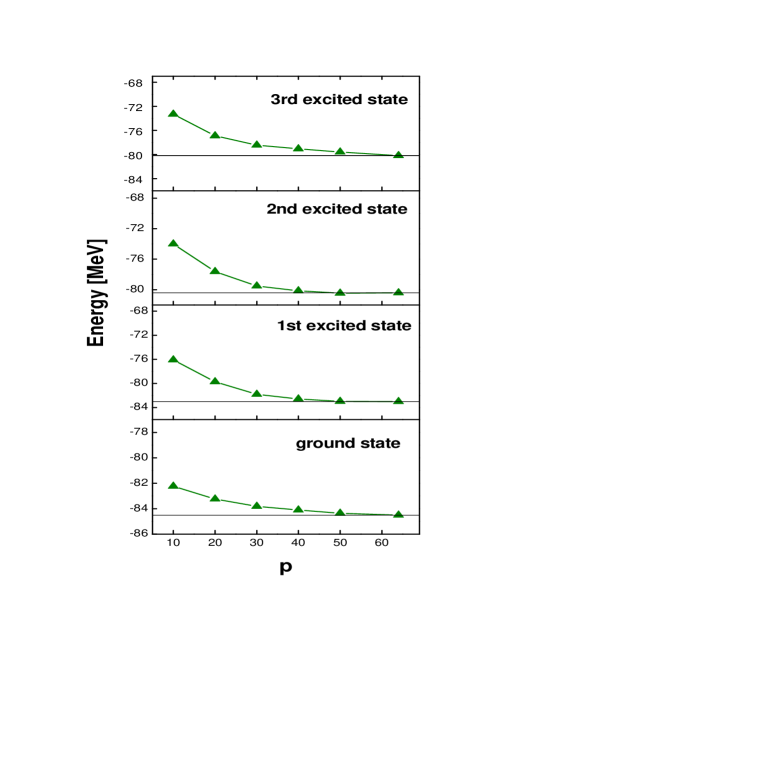
FIG. 4.: The energy of the ground state and of the three lowest excited states for ${}^{24}Mg$ as a function of $p$, the number of states retained in the block. The horizontal solid lines refer to the exact eigenenergy for each state.

Two points should be noted. First, the results indeed converge to the exact results for $p=64$, as they should. What is more important to note, however, is that the convergence is very slow. We need to have values of $p$ above $40$ to get reasonably accurate results when compared with the exact values. For the values of $p$ needed to get an accurate reflection of the full results we must treat hamiltonian matrices not much smaller than those of the full problem. Clearly, the method – as just described – is not working very well.

A What’s wrong?

From our perspective, there are at least two things wrong with the calculational framework that was used. On the one hand, since we worked in the m-scheme, we did not preserve angular momentum when we imposed truncation. If we want to work in the m-scheme and not lose angular momentum conservation we would have to (1) work in terms of spherical single-particle states, (2) include all states from a given orbit in a single step, and (3) make sure never to cut the truncation within a set of degenerate density matrix eigenvalues. This is possible, but extremely difficult, especially for systems with both neutrons and protons.

The second limitation of the method we employed is that it used the infinite algorithm and thus did not implement sweeping. As noted earlier, it is not practical to include sweeping in the p-h algorithm because of the preponderance of blocks that need to be coupled together. We have indeed implemented sweeping for ${}^{24}Mg$, and it did improve the results slightly, but it is clear that this is not the way to proceed for more complex nuclei.

IV What next?

Based on these considerations, we now believe that the minimum requirements for a useful DMRG strategy in nuclear physics are (1) that it works in a J-scheme or angular momentum conserving basis and (2) that it implements sweeping. In the following subsection, we sketch how this can be done. Further discussion of symmetry-conserving DMRG methods can be found in ref. [10].

A The J-DMRG

1 Initialization

We will illustrate the J-DMRG method through a problem involving five neutron orbits and five proton orbits, as illustrated in figure 5. These are spherical shell-model orbits, with definite $n$, $l$ and $j$. However, we only show $j$ for simplicity.

$j_{5\quad}\_\_\_\_\quad$ $\quad\_\_\_\_\quad j_{10}$ $j_{4\quad}\_\_\_\_\quad$ $\quad\_\_\_\_\quad j_{9}$ $j_{3\quad}\_\_\_\_\quad$ $\quad\_\_\_\_\quad j_{8}$ $j_{2}\quad\_\_\_\_\quad$ $\quad\_\_\_\_\quad j_{7}$ $j_{1\quad}\_\_\_\_\quad$ $\quad\_\_\_\_\quad j_{6}$ $\nu$ $\pi$

FIG. 5.: Active single-particle levels for the discussion of the J-DMRG method in the text.

Input to the calculation includes the number of neutrons and protons, the shell-model hamiltonian, including one- and two-body terms, and a set of single-shell matrix elements for each active orbit.

The single-shell matrix elements are the reduced matrix elements of all sub-operators of the hamiltonian within the orbit. All can be readily obtained from the Coefficients of Fractional Parentage for the orbit. Such single-shell reduced matrix elements are a common feature of all J-scheme shell model codes.

2 The warm-up phase

The next step is the warm-up phase, in which we carry out a first pass through the orbits and store an initial set of reduced matrix elements associated with the various possible blocks (groups of orbits). This includes for neutrons the orbits $j_{1}\rightarrow j_{2}$, $j_{1}\rightarrow j_{3}$, $j_{1}\rightarrow j_{4}$ and $j_{1}\rightarrow j_{5}$, with corresponding blocks for protons.

$j_{5\quad}\_\_\_\_\quad$ $\quad\_\_\_\_\quad j_{10}$ $j_{4\quad}\_\_\_\_\quad$ $\quad\_\_\_\_\quad j_{9}$ $j_{3\quad}\_\_\_\_\quad$ $\quad\_\_\_\_\quad j_{8}$ $j_{2}\quad\_\_\_\_\quad$ $\quad\_\_\_\_\quad j_{7}$ $j_{1\quad}\_\_\_\_\quad$ $\quad\_\_\_\_\quad j_{6}$ $\nu$ $\pi$

FIG. 6.: Schematic illustration of the warm-up phase of the J-DMRG method for finite fermi systems. The lowest two neutron levels form a neutron block and the lowest two proton levels a proton block.

Consider for example the schematic illustration shown in figure 6. At this point, we have treated the first two orbits for both neutrons and protons. In each of the two blocks, we have a given number of states with each $n$ (the total number of particles) and $J$ (the total angular momentum). The number of states is analogous to the quantity $p$ introduced earlier. Furthermore, in the two blocks the reduced matrix elements of all sub-operators of the hamiltonian have already been stored.

We then add the next neutron level, as illustrated in figure 7.

$j_{5\quad}\_\_\_\_\quad$ $\quad\_\_\_\_\quad j_{10}$ $j_{4\quad}\_\_\_\_\quad$ $\quad\_\_\_\_\quad j_{9}$ $j_{3\quad}\_\_\_\_\quad$ $\quad\_\_\_\_\quad j_{8}$ $j_{2}\quad\_\_\_\_\quad$ $\quad\_\_\_\_\quad j_{7}$ $j_{1\quad}\_\_\_\_\quad$ $\quad\_\_\_\_\quad j_{6}$ $\nu$ $\pi$

FIG. 7.: Schematic illustration of the enlargement of the neutron block of figure 6 in the warm-up phase of the J-DMRG method.

To do so, we first construct states of good angular momentum for the enlarged neutron block. We then calculate the matrix elements of all neutron operators in the enlarged neutron block, using standard formulae given for example in ref. [11]. The calculation requires reduced matrix elements from the block made up of orbits $j_{1}$ and $j_{2}$, which were stored in the previous iteration, and those of the orbit $j_{3}$ , which were stored in the input stage.

We then couple neutrons and protons together to states of good angular momentum, calculate the hamiltonian matrix in this basis and diagonalize. We then construct the ground state density matrix for neutrons and use it to truncate to the same number of states as we had before level $j_{3}$ was added. Then we transform all reduced matrix elements to the truncated block and store them.

And then we add the next proton level, and then the next neutron level, etc, until all levels have been included. At that point we have a first guess as to the optimum states associated with the successively larger blocks of levels.

3 The sweeping phase

We now turn to the sweeping phase, schematically illustrated in figure 8. It is during this phase that we systematically improve our description of the physics of each of the blocks, by taking into account the influence of the other orbits in the problem.

The idea of the picture is as follows. We have just treated the block of proton orbits $j_{9}$ and $j_{10}$. We now wish to add to it the proton orbit $j_{8}$ to create an enlarged proton block. We will carry out a truncation in this enlarged block, following the density matrix strategy. To do so, we consider the block $j_{6}\rightarrow j_{7}$ as the proton medium and the block $j_{1}\rightarrow j_{5}$ as the neutron medium. We then couple the states of the enlarged proton block to the two parts of the medium to obtain the superblock, an approximation to the entire system. We calculate the hamiltonian in the associated superblock, using only stored information We then diagonalize the superblock hamiltonian and determine the density matrix for the enlarged proton block, orbits $j_{8}\rightarrow j_{10}$. We then use this to truncate the enlarged proton block to the same number of states as we had before enlarging it. Then, we calculate all reduced matrix elements in the truncated proton block and store them. And then we add the next orbit, $j_{7}$. We do this for all proton blocks and then for all neutron blocks. And after the sweep is finished, we simply turn around and sweep upwards, continuing the process until the results from one sweep and those from the previous sweep are acceptably close.

$j_{5\quad}\_\_\_\_\quad$ $\quad\_\_\_\_\quad j_{10}$ $j_{4\quad}\_\_\_\_\quad$ $\quad\_\_\_\_\quad j_{9}$ $j_{3\quad}\_\_\_\_\quad$ $\quad\_\_\_\_\quad j_{8}$ $j_{2}\quad\_\_\_\_\quad$ $\quad\_\_\_\_\quad j_{7}$ $j_{1\quad}\_\_\_\_\quad$ $\quad\_\_\_\_\quad j_{6}$ $\nu$ $\pi$

FIG. 8.: Schematic illustration of the sweeping phase of the J-DMRG algorithm. We are sweeping downwards in protons, having treated as a block the levels $j_{9}$ and $j_{10}$. The level $j_{8}$ is then to be added to the block, and the enlarged block is treated in a medium involving the proton block $j_{6}\rightarrow j_{7}$ and the neutron block $j_{1}\rightarrow j_{5}$ from the previous sweep.

The formalism, as just described, is in the process of being implemented by two of the authors (SP and JD) in collaboration with Nicu Sandulescu and Larisa Pacearescu.

V Closing Remarks

In this presentation, we have provided a status report on recent efforts to develop the Density Matrix Renormalization Group method for use in large-scale nuclear shell-model calculations. Following a brief review of the general ideas behind the DMRG, we described the first application of the p-h variant of the method to realistic nuclei. Regrettably, the results were not especially promising. We discussed some of the reasons for the failure and then discussed a possible strategy that might overcome those shortcomings. The basic idea is to implement the DMRG algorithm in an angular-momentum-conserving basis and to include sweeping. While we are guardedly optimistic that this will indeed provide a practical and efficient methodology for large-scale nuclear structure calculations of heavy nuclei, only time will tell.

Acknowledgments This work was supported in part by the US National Science Foundation under grant #s PHY-9970749 and PHY-0140036, by the Spanish DGI under grant BFM2000-1320-C02-02, by NATO under grant PST.CLG.977000, and by the Bulgarian National Foundation for Scientific Research under Contract # $\Phi$-809. One of the authors (SP) wishes to acknowledge fruitful discussions on the J-DMRG method with Nicu Sandulescu.

REFERENCES

- [1] S. R. White, Phys. Rev. Lett. 69, 2863 (1992); S. R. White, Phys. Rev. B48, 10345 (1993); S. R. White and D. A. Huse, Phys. Rev. B48, 3844 (1993).
- [2] Density Matrix Renormalization, edited by I. Peschel, X. Xiang, M. Kaulke and K. Hallberg, Lectures Notes in Physics, (Springer. Berlin, 1999); S. R. White, Phys. Rep. 301, 187 (1998).
- [3] T. Xiang, Phys. Rev. B53 (1996) R10445.
- [4] S. R. White and R. L. Martin, J. Chem. Phys. 110, 4127 (1999).
- [5] S. Daul, I. Ciofini, C. Daul and S. R. White, Int. J. Quantum Chem. 79, 331 (2000); A. O. Mitrushenko, G. Fano, F. Ortolani, R. Linguerri and P. Palmeri, J. Chem. Phys. 115; G. Fano, F. Ortolani and L. Ziosi, J. Chem. Phys. 108, 9246 (1998); L. Bendazzoli, S. Evangelisti, G. Fano, F. Ortolani and L. Ziosi, J. Chem. Phys. 109, 1277 (1999) 6815 (2001); G. K-L. Chan and M. Head-Gordon, J. Chem. Phys. 116 4462 (2002).
- [6] J. Dukelsky and G. Sierra, Phys. Rev. Lett. 83, 172 (1999); J. Dukelsky and G. Sierra, Phys. Rev. B61, 12302 (2000).
- [7] J. Dukelsky and S. Pittel, Phys. Rev. C63, 061303(R) (2001); J. Dukelsky, S. Pittel, S.S. Dimitrova, M.V. Stoitsov, Phys. Rev. C65, 054319 (2002).
- [8] S. Pittel and J. Dukelsky, Rev. Mex. de Física 47 Suppl. (2001) 42.
- [9] K. G. Wilson, Rev. Mod. Phys. 47, 773 (1975).
- [10] Ian P. McCulloch and Miklós Gulácsi, Europhys. Lett. 57, 852 (2002)
- [11] A. de-Shalit and I. Talmi, Nuclear Shell Theory, (Academic Press, New York, 1963).