Non-Linear Vibrations in Nuclei

Abstract

We have performed Time Dependent Hartree Fock (TDHF) calculations on the non linear response of nuclei. We have shown that quadrupole (and dipole) motion produces monopole (and quadrupole) oscillations in all atomic nuclei. We have shown that these findings can be interpreted as a large coupling between one and two phonon states leading to strong anharmonicities.

]

I Introduction

Fifty years ago, it was discovered that atomic nuclei may enter in resonance with electromagnetic fields[1]. This Giant Dipole Resonance (GDR) has been interpreted as the vibration of neutrons against protons. Since then, other giant resonances (GR) have been predicted and observed, e.g. the Monopole GR (GMR), an alternation of compression and decompression of the nucleus, and the Quadrupole GR (GQR), an oscillation between a prolate and an oblate shape. The proof of the vibrational nature of the GR came only few years ago with the observation of the second vibrational quantum called the two-phonon state[2, 3]. While many properties of these states plead in favor of an harmonic picture, striking experimental observations such as an abnormally large excitation probability point to a strong coupling between the different phonon states[4, 5]. This triggered a lot of theoretical investigations but only very weak anharmonicities were found[6, 7, 8, 9, 10, 11] creating an important crisis in our understanding of nuclear vibrations.

Recently, it has been proposed that a strong anharmonicity may come from large residual interaction leading to the excitation of a GMR and a GQR on top of any state [12]. This was a surprise especially in the monopole case since it was generally believed that these couplings were small because of cancellation effects between various diagrams [13]. It is shown in reference [12] that these cancellations between 3-particle 1-hole and 3-hole 1-particle matrix elements were very limited. However, the approach of [12] even if it is fully microscopic do have some drawbacks. It is based on boson mapping methods which may lead to violation of the Pauli principle and mixing with the spurious states[14]. Therefore, an independent confirmation of these important couplings leading to the excitation of a GMR and GQR on top of phonon states is crucial.

In parallel looking to a completely different process, the excitation of a GDR in fusion reactions, we have shown [15] that, in a time dependent Hartree Fock (TDHF) approach, the dipole mode is non linearly coupled with other collective modes such as in particular the vibration of the density around a prolate shape. This work is also pointing in the direction of anharmonic vibrations in nuclei but the particularities of the fusion dynamics and of the composite system does not allow to draw conclusions about the properties of the phonon built on the ground state.

In this work, we present the first realistic TDHF calculation [16] of non-linear response to the collective vibrations showing that, indeed, the one- to two- phonon coupling is a source of anharmonicities. We used the TDHF approach [17, 18, 19, 16, 20] which corresponds to an independent propagation of individual particles in the self-consistent mean field generated collectively. It does not incorporate the dissipation due to two-body interaction [21, 22, 23], but takes into account one body mechanisms such as Landau spreading and evaporation damping [24]. The quantal nature of the single particle dynamics is explicitly preserved, which is crucial at low energy both because of shell effects and of the wave dynamics. In its small amplitude limit TDHF is equivalent to the Random Phase Approximation (RPA) which is the basic tool to understand the collective response of nuclei in terms of independent phonons. However, since the mean-field depends upon the actual excitation, TDHF is a non linear theory and hence contains couplings between collective modes. This point will be explicitly developed in the following. In fact TDHF is optimized for the prediction of the average value of one body observables. Through non-linearities, it takes into account the effects of the residual interaction as soon as the considered phenomenon can be observed in the time evolution of a one body observable. Of course, the absence of terms explicitly taking into account the correlations is a limitation. In particular, dampings and spreadings are neglected. As far as the time dependent approaches are concerned, it would be important to extend the present study to theories going beyond the one body limit such as extended TDHF [23] which incorporate the effect of a ”collision term” and also, through the fluctuations associated with the considered dissipation, the coherent coupling with phonon plus particle hole excitations. Even more complete theories such as the time dependent density matrix approach[10, 25], which is known to reduce to the second RPA in its linearized version, would be an interesting extension of the present work. Finally, one should also try to apply the stochastic mean field approaches in particular in its version which have been proved to be potentially an exact solution of the many-body problem[26]. However, the analysis presented in section 3 clearly show that the non linear response in TDHF contains the couplings between one and two phonon states coming from the 3-particle 1-hole and 1-particle 3-hole residual interaction.

In section 2 we demonstrate first that coupling between one and two phonon states can be obtained through the evolution of average values of one-body observables. In section 3, we show which part of the residual interaction is taken into account in a TDHF approach. In section 4 we present results demonstrating the importance of the non-linear excitation of monopole and quadrupole modes on top of other collective vibrations. Finally we will conclude in section 5.

II Effect of couplings on one-body observables

To understand how this coupling can be extracted from the one-body dynamics let us consider the nonlinear coupling of a mode, $\mid\nu>$ with the GR$\mu$ built on top of it leading to the two phonon state $\mid\nu\mu>$. The Hamiltonian can be written

$\displaystyle{H}={H}_{0}+{V}$

where ${H}_{0}$ corresponds to the harmonic (RPA) part for which $\mid\nu>$ and $\mid\nu\mu>$ are eigenstates with energies $\omega_{\nu}$ and $\omega_{\nu\mu}=$ $\omega_{\nu}+$ $\omega_{\mu}$ while ${V}$ is the residual interaction between phonons. For simplicity, let us introduce only the non-linear coupling $v_{\mu}=<\nu\mid{V}\mid\nu\mu>$ which has been proven to be the most important one[12]. At the first order in $\varepsilon=v_{\mu}/\omega_{\mu}$, this leads to the eigen states :

$\displaystyle\mid\overline{\nu}>=({\mid\nu>-\varepsilon\mid\nu\mu>})/{\mathcal{N}}$

and

$\displaystyle\mid\overline{\nu\mu}>=({\varepsilon\mid\nu>+\mid\nu\mu>})/{\mathcal{N}}$

where ${\mathcal{N}}^{2}={{1+\varepsilon^{2}}}$. A collective boost

$\displaystyle\mid\psi(t=0)>=e^{-ik_{\nu}{Q}_{\nu}}\mid->$

inducing transitions between the ground state $\mid->$ and the collective state $\mid\nu>$ with the amplitude $q_{\nu}=<-\mid{Q}_{\nu}\mid\nu>$, leads to

$$\mid\psi(t)>\simeq\mid->-ik_{\nu}q_{\nu}e^{-i\omega_{\nu}t}(\mid\overline{\nu}>-e^{-i\omega_{\mu}t}\varepsilon\mid\overline{\nu\mu}>).$$ (1)

Then, $<{Q}_{\nu}>(t)$ is simply given by

$$<{Q}_{\nu}>(t)\simeq-2k_{\nu}q_{\nu}^{2}\sin(\omega_{\nu}t).$$ (2)

This shows that the linear response to collective boost induces oscillation of the collective moment at the collective frequency with an amplitude proportional to the transition probability $q_{\nu}^{2}.$ If we now compute the response to the operator ${Q}_{\mu}$ which is associated with the excitation of the giant resonance $\mu,$ it is not zero because of the transitions between $\mid\overline{\nu}>$ and $\mid\overline{\nu\mu}>.$ Using Eq. (1) and assuming $<\nu\mu\mid{Q}_{\mu}\mid\nu>=q_{\mu}$ too, we get at the lowest order in $k_{\nu}$ and $v/\omega_{\mu}$

$$\,<{Q}_{\mu}>(t)=2k_{\nu}^{2}q_{\nu}^{2}q_{\mu}\frac{v_{\mu}}{\omega_{\mu}}\left(\cos(\omega_{\mu}t)-1\right)$$ (3)

where the $-1$ term comes from higher order terms not explicitly written in Eq. (1). This demonstrates that the induced moment $<{Q}_{\mu}>\left(t\right)$ is quadratic in the collective boost amplitude as expected from its non linear nature. Moreover, it oscillates at the frequency of the coupled mode $\omega_{\mu}$ with an amplitude proportional to the mixing coefficient $v_{\mu}/\omega_{\mu}$ and to the matrix element $q_{\mu}.$ Finally, it should be noticed that $<{Q}_{\nu}>(t)$ and $<{Q}_{\mu}>(t)$ start in phase quadrature.

III Linear and non-linear response in TDHF

The TDHF approach is built to describe the average values of one-body observables. It propagates the evolution of the one-body density matrix

$\displaystyle{\rho}_{ij}=<a_{j}^{+}a_{i}>$

where $a_{i}^{+}$ is the operator creating a particle in the orbital $|i>$:

$\displaystyle i\partial_{t}\rho=[h,{\rho}]$

where ${h}$ is the self-consistent mean-field Hamiltonian linked to the mean field energy $E$ by ${h}_{ij}=\partial E/\partial{\rho_{ji}}$ . We have used the code of ref. [27] with $SGII$ [28] and $SLy4d$ [29] Skyrme interactions.

The RPA can be obtained by the linearization of the TDHF equation. Let us now go beyond the RPA by expanding the one-body density $\rho$ up to the quadratic terms in the collective boost strength $k_{\nu}$:

$\displaystyle\rho=\rho^{(0)}+k_{\nu}\rho^{(1)}+k_{\nu}^{2}\rho^{\left(2\right)}.$

$\rho^{(0)}$, the static HF groundstate, defines the occupied states ($h$) ${\rho}^{(0)}=\sum_{h=1}^{A}\left|\varphi_{h}><\varphi_{h}\right|$, the unoccupied states being the particle states ($p$). The condition on the one-body density $\rho$ due to the independent particle approximation made when deriving the TDHF equation leads to the constrain $\rho^{2}=\rho$. This imposes that $\rho^{(1)}$ contains only $p$-$h$ components which directly provide the particle-particle and hole-hole elements of the quadratic term of the one-body density

$\displaystyle\rho_{pp^{\prime}}^{(2)}=\sum_{h}\rho_{ph}^{(1)}\rho_{hp^{\prime}}^{(1)}$

and

$\displaystyle\rho_{hh^{\prime}}^{(2)}=-\sum_{p}\rho_{hp}^{(1)}\rho_{ph^{\prime}}^{(1)}.$

A TDHF and RPA

The linear part of the TDHF equation leads to

$\displaystyle i\partial_{t}{\rho}^{(1)}={{\mathcal{M}}}\rho^{(1)}$

where

$\displaystyle{\mathcal{M}}\cdot=[h^{(0)},\cdot]+[\frac{\partial h}{\partial\rho}\cdot,\rho^{\left(0\right)}]$

is nothing but the RPA matrix acting only in the ph space. The RPA response after a boost $e^{-ik_{\nu}Q_{\nu}}$ at time $t=0$ with $Q_{\nu}=q_{\nu}O_{\nu}^{+}+h.c.$ where

$\displaystyle\rho_{\nu}^{+}=[O_{\nu}^{+},\rho^{\left(0\right)}]$

is the RPA mode associated with the frequency $\omega_{\nu}$, is

$\displaystyle\rho^{(1)}=-q_{\nu}\rho_{\nu}^{+}ie^{-i\omega_{\nu}t}+h.c.\;.$

Using $\mathrm{Tr}O_{\nu}\rho_{\nu^{\prime}}^{+}=\delta_{\nu\nu^{\prime}}$, we get

$\displaystyle<Q_{\nu}>=-2q_{\nu}^{2}k_{\nu}\sin\omega_{\nu}t$

which corresponds to Eq. (2) and explain why the RPA provides a good approximation of $\omega_{\nu}$ and $q_{\nu}^{2}$.

B Quadratic response and phonon coupling

If we now compute the quadratic response in the TDHF approximation, we get for $\bar{\rho}^{(2)}$, the $p-h$ component of the one-body density $\rho^{(2)}$

$$i\partial_{t}\bar{\rho}^{(2)}={\mathcal{M}}\bar{\rho}^{(2)}+V^{d}+V^{e}+\delta V$$ (4)

where the three sources of non linearities are the $p-h$ components of

$$\delta V = \frac{1}{2}[\sum_{ijkl}\frac{\partial^{2}h}{\partial\rho_{ij}\partial\rho_{kl}}\rho_{ij}^{(1)}\rho_{kl}^{\left(1\right)},\rho^{\left(0\right)}]$$

$$V^{d} = [\sum_{ij}\frac{\partial h}{\partial\rho_{ij}}\rho_{ij}^{(1)},\rho^{\left(1\right)}]$$

$$V^{e} = [\sum_{ijk}\frac{\partial h}{\partial\rho_{ij}}\varepsilon_{i}\rho_{ik}^{(1)}\rho_{kj}^{(1)},\rho^{\left(0\right)}]$$

where $\varepsilon_{p}=1$ and $\varepsilon_{h}=-1$ and . It should be stressed that Eq. (4) is of course not the more general one but has the merit to be derived within the well defined framework of the time dependent mean field approximation. The $p-h$ component of $\rho^{(2)}$ can be expanded on the RPA basis

$\displaystyle\bar{\rho}^{(2)}=q_{\nu}^{2}\sum_{\mu}z_{\mu}\rho_{\mu}^{+}+h.c.$

where we have explicitly factorized the transition probability $q_{\nu}^{2}$. Using $\mathrm{Tr}O_{\mu}\rho_{\mu^{\prime}}^{+}=\delta_{\mu\mu^{\prime}}$, the evolution of $z_{\mu}$ can be isolated:

$\displaystyle i\dot{z}_{\mu}=\omega_{\mu}z_{\mu}+v_{\mu}^{d}+v_{\mu}^{e}+\delta v_{\mu}$

with

$\displaystyle v_{\mu}^{d}=\mathrm{Tr}O_{\mu}V^{d}/q_{\nu}^{2},v_{\mu}^{e}=\mathrm{Tr}O_{\mu}V^{e}/q_{\nu}^{2}$

and

$\displaystyle\delta v_{\mu}=\mathrm{Tr}O_{\mu}\delta V/q_{\nu}^{2}.$

The time independent parts of $v_{\mu}^{d}+v_{\mu}^{e}$ $+\delta v_{\mu}$ , $v_{\mu}$, lead to

$\displaystyle z_{\mu}=\frac{v_{\mu}}{\omega_{\mu}}(e^{-i\omega_{\mu}t}-1)$

so that

$\displaystyle<Q_{\mu}>=2k_{\nu}^{2}q_{\mu}\frac{q_{\nu}^{2}v_{\mu}}{\omega_{\mu}}\left(\cos\omega_{\mu}t-1\right).$

Comparing this result with the Eq. (3) shows that $v_{\mu}$ can be interpreted as the residual interaction exciting, in TDHF, the mode $\mu$ on top of the phonon $\nu$.

C Link with the residual interaction

To illustrate this coupling, let us compute the contribution coming from the forward amplitudes $\rho_{\nu_{ph}}^{+}=O_{\nu_{ph}}^{+}=X_{ph}^{\nu}$ then $v_{\mu}^{d}$ contains two terms involving the $3p-1h$ and $3h-1p$ residual interaction,

$$v_{\mu}^{d} = \sum V_{p^{\prime}h^{\prime\prime};pp^{\prime\prime}}X_{ph}^{\mu}X_{p^{\prime\prime}h^{\prime\prime}}^{\nu}X_{p^{\prime}h}^{\nu}$$ (6)

$$-\sum V_{hh^{\prime\prime};h^{\prime}p^{\prime\prime}}X_{ph}^{\mu}X_{p^{\prime\prime}h^{\prime\prime}}^{\nu}X_{ph^{\prime}}^{\nu}$$

where we have introduced $V_{ik;jl}={\partial h_{ji}}/{\partial\rho_{kl}}$. Considering the second term $v_{\mu}^{e}$ we get also two components

$$v_{\mu}^{e} = \sum V_{p^{\prime}h^{\prime\prime};pp^{\prime\prime}}X_{p^{\prime\prime}h^{\prime\prime}}^{\mu}X_{ph}^{\nu}X_{p^{\prime}h}^{\nu}$$ (8)

$$-\sum V_{hh^{\prime\prime};h^{\prime}p^{\prime\prime}}X_{p^{\prime\prime}h^{\prime\prime}}^{\mu}X_{ph^{\prime}}^{\nu}X_{ph}^{\nu}$$

which are nothing but the exchange of $\mu$ and $\nu$ in $v_{\mu}^{d}$. These four terms correspond exactly to the $X$ part of the phonon interaction $\left\langle\mu\nu\right|V\left|\nu\right\rangle$ computed using boson mapping [12] except for a numerical factor which actually depends upon the mapping used.

The $X$ part of $\delta v_{\mu}$ is $\sum\frac{\partial V_{h^{\prime\prime}p^{\prime};p^{\prime\prime}h^{\prime}}}{\partial\rho_{ph}}X_{ph}^{\mu}X_{p^{\prime}h^{\prime}}^{\nu}X_{p^{\prime\prime}h^{\prime\prime}}^{\nu}$. It results from the density dependence of the $p-h$ interaction defining the energy of the state $\nu$. In the simple case of a linear density dependence, it can be interpreted as a contribution of a three-body interaction inducing transitions from $1p-1h$ to $2p-2h$.

This analysis clearly shows that the time dependence in TDHF takes into account the residual interaction. At the linear level, TDHF leads to the RPA. Going to the quadratic response, TDHF takes into account the one- to two-phonon coupling. The key point of the applicability of TDHF is the fact that the studied phenomenon can be deduced from the time dependence of the average value of a one-body observable.

IV Results

Let us now look at the TDHF results for the ${}^{40}Ca$ nucleus. We followed the monopole, quadrupole and dipole response for three initial conditions:

• A monopole boost using

  
  

  $\displaystyle{Q}_{0}=\frac{1}{\sqrt{4\pi}}\sum_{i}({r}_{i}^{2}-<{r}_{i}^{2}>(t=0)).$

  because of the spherical symmetry, a monopole boost can only trigger monopole modes. Therefore, we only observe $<{Q}_{0}>(t).$

• A quadrupole boost generated by

  
  

  $\displaystyle{Q}_{2}=\sum_{i}{r}_{i}^{2}Y_{0}^{2}\left({\theta}_{i},{\varphi}_{i}\right).$

  The parity conservation forbids any dipole excitation when a quadrupole velocity field is applied to a spherical nucleus. Conversely, breathing modes (GMR) can be triggered by the quadrupole oscillation so that we do follow both the quadrupole $<{Q}_{2}>(t)$ and the monopole $<{Q}_{0}>(t)$ responses.

• An isovector dipole boost induced by

  
  

  $\displaystyle{Q}_{D}=Z/A\sum_{n}z_{n}-N/A\sum_{p}z_{p}.$

  This excitation can be both coupled to the quadrupole and monopole oscillations so that we monitor the three moments, $<{Q}_{0}>(t)$, $<{Q}_{2}>(t)$ and $<{Q}_{D}>(t).$

FIG. 1.: Evolutions of the monopole, quadrupole and dipole moments (solid lines) and of the central density $\rho_{0}$ (dashed lines) as a function of time for monopole (a), quadrupole (b) and dipole (c) excitations in ${}^{40}Ca$.

In figure 1, we observe that the collective boost induces oscillations of the associated moment as expected from the RPA (see Eq. (2)). They are only slightly damped in the GQR and GDR cases (fig. 1-b and 1-c respectively) while in the GMR case (fig. 1-a) beatings, characteristic of a Landau damping, are observed. This means that the dipole and quadrupole strengths are mostly concentrated in a single resonance while the monopole one is fragmented.

Plotting in figure 2 the amplitude of the first oscillation $<{Q}_{\nu}>_{max}$ as a function of $k_{\nu}$ confirms the linearity of this response. Assuming that only one mode is excited which is a good approximation for the GDR and GQR (Eq. (2)) shows that the transition probability, $q_{\nu}^{2},$ is $<{Q}_{\nu}>_{max}/2k_{\nu}.$ To get a deeper insight into the response we study the Fourier transform $F(\omega)$ of $<{Q}_{\nu}>(t)/k_{\nu}$ which is nothing but the RPA strength when the velocity field $k_{\nu}$ is small enough to be in the linear regime. We see in figure 3 that the dipole and quadrupole modes are concentrated in a unique mode while the monopole is fragmented. However, the various peaks are in the same energy region so that they can be approximated by a single mode with a large Landau width. A detailed test of the equivalence between the linear regime of TDHF and the RPA response can be found in [24].

If we now turn to the non linearities, we can observe the moments ${Q}_{\mu}$ which are different from the operator ${Q}_{\nu}$ used for the exciting boost. We see in figure 1 that, as expected from Eq. (3), this non linear response follows a $\left(\cos(\omega_{\mu}t)-1\right)$ pattern oscillating with the frequency of the mode $\mu$ and not the one of the initially excited collective state $\nu$. Moreover the amplitude of the first oscillation (fig. 2) is as expected quadratic in the excitation velocity $k_{\nu}$. In Fig. 1, one can see that large amplitude dipole (fig. 1-c) and quadrupole (fig. 1-b) motion induces variations of the central density $\rho_{0}$. Since the central density can be modified only by monopole states this imposes that the large amplitude motion gets coupled with such breathing modes. In the same way a large amplitude dipole oscillation induces a quadrupole deformation of the nuclear potential and so gets coupled with the GQR. These observations lead to the conclusion that we are in the presence of a non-linear excitation of a giant resonance $\mu$ on top of the collective motion $\nu$ initially excited through the collective boost ${Q}_{\nu}$.

FIG. 2.: Evolutions of the maximal oscillation amplitudes of $<{Q}_{0}>$ (solid line), $<{Q}_{2}>$ (dashed line) and $<{Q}_{D}>$ (dotted line) as a function of the intensities of the monopole (a), quadrupole (b), and dipole excitations (c). The horizontal lines represent the average number of excited phonons for each GR.

The Fourier transform of $<{Q}_{\mu}>(t)$ associated with the excitation of ${Q}_{\nu}$ are also presented in figure 3. Let us first start with the quadrupole strength non-linearly excited by a dipole boost. This is a clear indication that the observed state is indeed a GQR built on top of the GDR. This is what is expected from Eq. (3) where only the frequency $\omega_{\mu}$ of the observed state appears. It should be notice that this frequency is different from one of the underlying dipole motion. The monopole case is more complex because of the presence of a strong Landau spreading and it seems that the strengths of the various monopole states depend upon the considered boost. This indicates that the coupling leading to the excitation of an additional monopole state depends upon the collective mode initially excited.

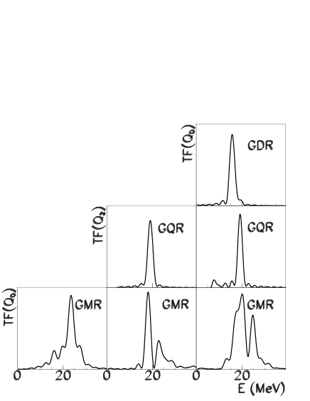
FIG. 3.: Monopole, quadrupole and dipole spectra (the Fourier transforms are in arbitrary units) for a monopole (left), quadrupole (middle) and dipole excitation (right).

To estimate the magnitude of these non-linear couplings, we can first convert the amplitude of the induced oscillations into a phonon number using a coherent state picture. The horizontal lines in figure 2 represent the amplitude of the oscillations associated with different number $<{n}_{\nu}>=1,2,3,...$ of excited phonons:

$\displaystyle<{Q}_{\nu}>_{max}^{2}=4<{n}_{\nu}>q_{\nu}^{2}.$

One can see that for a $k_{\nu}$ which corresponds to the excitation of one phonon $\nu$ the number of phonons $\mu$ non-linearly excited is large.

Assuming for each multipolarity a unique state $|\mu>$ non linearly excited one can use Eq. (3) to extract the residual interaction matrix element $v_{\mu}$ between $|\nu>$ and $|\nu\mu>$ from the amplitudes of the induced oscillations $<{Q}_{\mu}>_{max}$

$$v_{\mu}={<{Q}_{\mu}>_{max}\omega_{\mu}}/{2k_{\nu}^{2}q_{\nu}^{2}q_{\mu}}.$$ (9)

If the non-linear collective response is not concentrated in a unique state $|\mu>$ but corresponds to a set of states $\{|\mu_{i}>\}$ with $\omega_{\mu_{i}}\approx\omega_{\mu}$, one can easily show that the extracted coefficient $v_{\mu}$ is related to the individual ${v_{\mu}}_{i}=<\nu|V|\nu\mu_{i}>$ by the weighted sum

$$v_{\mu}\approx\Sigma_{i}\sqrt{p_{\mu_{i}}}{v_{\mu}}_{i}$$ (10)

where $p_{\mu_{i}}=q_{\mu_{i}}^{2}/{\Sigma_{j}q_{\mu_{j}}^{2}}$ and $q_{\mu_{i}}=<-|Q_{\mu}|\mu_{i}>$. $v_{\mu}$ is in general higher than the individual ${v_{\mu}}_{i}$. For example, if the collective response is equally distributed into $N$ states with identical coupling matrix elements ${v_{\mu}}_{i}={\bar{v}_{\mu}}$ then $v_{\mu}=\sqrt{N}{\bar{v}_{\mu}}$.

$|\nu>$	$\omega_{\nu}$	$q_{\nu}$	$S_{1}$	$<\nu|{V}|\nu 0>$	$<\nu|{V}|\nu 2>$
	$(MeV)$			$(MeV)$	$(MeV)$
$|0>_{{}^{40}Ca}$	$22.9$	$11.6$	$3090$		$0$
$|2>_{{}^{40}Ca}$	$18.6$	$21.4$	$9020$	$-4.28$
$|D>_{{}^{40}Ca}$	$17.2$	$3.47$	$199$	$-4.58$	$-3.92$
$|0>_{{}^{90}Zr}$	$19.9$	$26.0$	$12900$		$0$
$|2>_{{}^{90}Zr}$	$15.0$	$46.5$	$35700$	$-2.55$
$|D>_{{}^{90}Zr}$	$14.4$	$5.44$	$442$	$-1.60$	$-1.93$
$|0>_{{}^{208}Pb}$	$15.7$	$57.1$	$51200$		0
$|2>_{{}^{208}Pb}$	$11.1$	$99.0$	$128000$	$-2.17$
$|D>_{{}^{208}Pb}$	$13.0$	$8.94$	$877$	$-2.40$	$-0.70$

TABLE I.: Energies, transition probabilities $q_{\nu}$, energy weighted sum-rules $S_{1}$ and coupling coefficients of the GMR, GDR and GQR in the ${}^{40}Ca$, ${}^{90}Zr$ and ${}^{208}Pb$. $q_{\nu}$ and $S_{1}$ are expressed in $fm^{2}$ and $MeV.fm^{4}$ for the GMR and GQR and in $fm$ and $MeVfm^{2}$ for the GDR respectively.

The results for the ${}^{40}Ca$, ${}^{90}Zr$ and ${}^{208}Pb$ are presented in table 1. The $\omega_{\nu}$ are computed from the time to reach the first maximum of $<{Q}_{\nu}>(t)$. If the spreading of the observed mode is small, $\omega_{\nu}\approx{m_{2}}/{m_{1}}$ which should be a little higher than ${m_{1}}/{m_{0}}$ usually discussed. For the breathing mode, our results agree with the values obtained in [28] (${m_{1}}/{m_{0}}=22.7$, $19.5$, $15.3MeV$ in ${}^{40}Ca$, ${}^{90}Zr$ and ${208}Pb$ respectively). These RPA results as well as our $\omega_{\nu}$ are close to the averages which can be computed from the most collective states reported in ref. [12]. For the ${}^{40}Ca$, the ${m_{2}}/{m_{1}}$ for the monopole, quadrupole and dipole states of ref. [12] are respectively $21.2$, $16.9$ and $18.5$ $MeV$ for $84\%$, $85\%$ and $66\%$ of the corresponding energy weighted sum rules (EWSR). For ${208}Pb$ these values are $14.1$, $11.1$ and $13.6$ $MeV$ for $89\%$, $91\%$ and $80\%$ of the EWSR respectively. The relative sign of $v_{\mu}$ and $q_{\mu}$ is given by the early evolution of the moments described by Eq. (5) and shown in figure 1. They appear to be all negative in agreement with ref. [12]. The couplings $v_{\mu}$ are large of the order of few MeV. From the quantitative point of view, the non-linear coupling extracted from TDHF appears to be $50\%$ larger than the one reported in reference [12]. This is a reasonable agreement since TDHF result is a weighted sum of the individual couplings as shown in Eq. 10. Summing the contributions of the different collective states considered in ref. [12] reduces the difference between the reported values. However, the phonon basis studied in ref. [12] being incomplete it is expected that the TDHF results remains higher. It should be also noticed that some difference can remain due to the approximations involved in the different approaches as discussed in the quadratic response analysis.

In table 1 one can also see that the larger the nucleus the smaller the coupling. This is in agreement with the fact that these couplings are mediated by the surface. To control the robustness of our conclusion we have performed a series of calculations using a different Skyrme force, the recent SLy4d parametrization. For a ${}^{40}Ca$, this leads to a coupling exciting the GMR on top of the GDR of $-4.01$ $MeV$ and of $-4.36$ $MeV$ on top of the GQR. The quadrupole response during a dipole oscillation leads to a residual interaction of $-3.98$ $MeV.$ Those results are very close to the one reported in table 1.

V Conclusions

In conclusion, we have shown with TDHF calculations that a non-linear excitation of monopole and quadrupole should occur on top of any collective motion in nuclei. These couplings can be interpreted in terms of a large residual interaction which couples one-phonon and two-phonon states. These results show that large anharmonicities should be expected in the collective motions in nuclei.

We thank Paul Bonche for providing his TDHF code and helpful discussions. Comments and discussions with M. Andres, P.F. Bortignon, F. Catara, M. Fallot, J. Frankland, O. Juillet, D. Lacroix and E. Lanza are acknowledged.

REFERENCES

- [1] For a recent review see M.N. Harakeh and A. van der Woude (2001) Giant Resonances (Clarendon Press, Oxford).
- [2] Ph. Chomaz and N. Frascaria, Phys. Rep. 252, 275 (1995).
- [3] T. Aumann et al., Annu. Rev. Nucl. Sci. 48, 351 (1998).
- [4] C. Volpe et al., Nucl. Phys. A 589, 521 (1995).
- [5] P.F. Bortignon and C.H. Dasso, Phys. Rev. 56, 574 (1997).
- [6] V.Yu. Ponomarev, P.F. Bortignon, R.A. Broglia and V.V. Voronov, Phys. Rev. Lett. 85, 1400 (2000).
- [7] V.Yu. Ponomarev and P. Von Neumann-Cosel, Phys. Rev. Lett. 82, 501 (1999).
- [8] F. Catara, Ph. Chomaz and N. Van Giai, Phys. Rev. 48B, 18207 (1993).
- [9] E.G. Lanza, M.V. Andrés, F. Catara, Ph. Chomaz and C. Volpe, Nucl.Phys. A 613, 445 (1997).
- [10] M. Tohyama, Phys. Rev. C 64, 067304 (2001).
- [11] B. A. Brown, V. Zelevinsky and N. Auerbach, Phys. Rev. C 62, 044313 (2000).
- [12] M. Fallot et al, nucl-th/0111013, submitted.
- [13] J. Wambach, Rep. Prog. Phys. 51, 989 (1988).
- [14] D. Beaumel and Ph. Chomaz, Phys. Lett. B 277, 1 (1992).
- [15] C. Simenel, Ph. Chomaz and G. de France, Phys. Rev. Lett. 86, 2971 (2001).
- [16] P. Bonche, S. Koonin and J.W. Negele, Phys. Rev. C 13 , 1226 (1976).
- [17] D. R. Hartree, Proc. Camb. Phil. Soc. 24, 89 (1928).
- [18] V. A. Fock, Z. Phys. 61, 126 (1930).
- [19] D. Vautherin and D. M. Brink, Phys. Rev. C 5, 626 (1972).
- [20] J. W. Negele, Rev. Mod. Phys. 54, 913 (1982).
- [21] M. Gong, M. Toyama and J. Randrup, Z. Phys. A 335, 331 (1990).
- [22] C. Y. Wong and H. H. K. Tang, Phys. Rev. Lett. 40, 1070 (1978).
- [23] D. Lacroix, P. Chomaz and S. Ayik, Phys. Rev. C 58, 2154 (1998).
- [24] Ph. Chomaz, N. V. Giai and S. Stringari, Phys. Lett. B 189, 375 (1987).
- [25] S.J. Wang and W. Cassing, Ann. Phys. (N.Y.) 159, 328 (1985).
- [26] O. Juillet and Ph. Chomaz, Phys. Rev. Lett. 88, 142503 (2002).
- [27] K.-H. Kim, T. Otsuka, P. Bonche, J. Phys. G 23, 1267 (1997).
- [28] N.V. Giai and H. Sagawa, Nucl. Phys. A 371, 1 (1981).
- [29] E. Chabannat et al., Phys. Src. T 56, 31 (1995).