Spacelike and timelike response of confined relativistic particles

Abstract

Basic theoretical issues relating to the response of confined relativistic particles are considered including the scaling of the response in spacelike and timelike regions of momentum transfer and the role of final state interactions. A simple single particle potential model incorporating relativity and linear confinement is solved exactly and its response is calculated. The response is studied in common approximation schemes and it is found that final state interactions effects persist in the limit that the three-momentum transferred to the target is large. The fact that the particles are bound leads to a non-zero response in the timelike region of four-momentum transfer equal to about 10% of the total strength. The strength in the timelike region must be taken into account to fulfill the particle number sum rule.

1 Introduction

Deep inelastic scattering (DIS) of leptons by hadrons is generally discussed in the framework of the naive parton model and the QCD-improved parton model using the operator product expansion.ESW This approach has been very successful in determining the evolution of the structure functions as a function of the square of the four-momentum transferred to the hadron.AP77 In the leading order of the model the hadron is approximated by a collection of noninteracting quarks and gluons. The struck quark is assumed to be on the mass-shell both before and after its interaction with the electron. Basic theoretical considerations bring the validity of these assumptions into question.Bj00

Based on the assumption that the struck constituent is on the mass-shell before and after interaction with the probe, the response is predicted to be in the spacelike region for which the energy transfer $\nu$ is less than the magnitude of momentum transfer, $|\mathbf{q}|$, as a consequence of the inequality,

$$\nu=\sqrt{|\mathbf{k}+\mathbf{q}|^{2}+m_{q}^{2}}-\sqrt{|\mathbf{k}|^{2}+m_{q}^{2}}\leq|\mathbf{q}|.$$ (1)

Here $\mathbf{k}$ and $m_{q}$ are the momentum and mass of the struck quark, respectively. The predicted response is discontinuous at the boundary $|\mathbf{q}|=\nu$ between space and timelike regions. In fact interactions among the constituents in the initial state take the constituents off the mass-shell and move response of the target into the timelike region of four-momentum transfer.

In the many-body theory (MBT) one expects, at least naively, that final state interactions (FSI) should have an effect on inclusive scattering cross sections with electromagnetic probes from systems whose constituents are confined. Scattering of high energy probes from composite systems, such as electron scattering by nuclei Frois91 and nucleons ESW , or neutron scattering by liquid helium SS89 , is often used to study the structure of the bound system. The common assumption is that in DIS at sufficiently high energy the probe is incoherently scattered by the constituents of the system. In the plane wave impulse approximation (PWIA), which neglects FSI effects, DIS is directly related to the momentum and energy distribution of the constituents in the target.

The role of FSI effects has been studied extensively in electron scattering from nuclear targets BFFMPS91 ; BP93 and neutron scattering from liquid helium SS89 . Recently it has been suggested that they may also influence DIS of leptons by hadrons Brodsky . In the present study we focus on scattering from targets with confined constituents. The corresponding physical case concerns DIS from nucleons where, in distinction from the nuclear and liquid helium cases, the constituents are confined in both the initial and final states.

2 The response and scaling variables

We consider the response to a hypothetical scalar probe which couples to the density of a single scalar constituent. This allows us to ignore complications due to spin and the Lorentz structure of the response though it retains the qualitative features of a more realistic model where one considers the coupling of a spin-$\frac{1}{2}$ fermion to the conserved electromagnetic current. The response is

$$R(\mathbf{q},\nu)=\sum_{I}|\langle I|\sum_{j}e^{i\mathbf{q}\cdot\mathbf{r}_{j}}|0\rangle|^{2}\delta(E_{I}-E_{0}-\nu)$$ (2)

where $\sum_{j}$ is over all the particles and the $\sum_{I}$ over all energy eigenstates. It is viewed as the distribution of the strength of the state $\sum_{j}e^{i\mathbf{q}\cdot\mathbf{r}_{j}}|0\rangle$ over the energy eigenstates of the system having momentum $\mathbf{q}$. It is not necessarily zero in the timelike, $\nu>|\mathbf{q}|$ region.

2.1 Scaling variables

The conventional variables of the parton model, $Q^{2}=|\mathbf{q}|^{2}-\nu^{2}$ and the Bjorken $x=Q^{2}/2M\nu$, used to describe the DIS structure functions of a hadron of mass $M$, are confined to the spacelike region of the $|\mathbf{q}|$–$\nu$ plane for positive values of $Q^{2}$ accessible in lepton scattering experiments, as shown in Fig. 1. The observed ($Q^{2}>0$) DIS response is limited to a narrow region in the $|\mathbf{q}|-\nu$ plane illustrated in Fig. 1. It is bounded by the elastic limit, $\nu_{el}=\sqrt{|\mathbf{q}|^{2}+M^{2}}-M$ on one side, and by the photon line on the other. In the limit of large $|\mathbf{q}|$ the width of the observed response at fixed $|\mathbf{q}|$ is $M$. Lines of constant $Q^{2}$ intersect the elastic limit curve at $x=1$ and approach the photon line at small $x$.

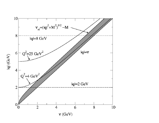
Figure 1: The $|\mathbf{q}|$-$\nu$ plane. The spacelike region is above the $|\mathbf{q}|=\nu$ line and timelike is below. Lines of constant $Q^{2}>0$ are parabolas which lie entirely in the spacelike region and approach $|\mathbf{q}|=\nu$ as $\nu\rightarrow\infty$. The observed ($Q^{2}>0$) response of the proton lies in the shaded area.

We wish to study the full range of response possible for a system of bound constituents including the region of timelike momentum transfer. Therefore we study the response, $R(\mathbf{q},\nu)$ as a function of $\nu$ and $|\mathbf{q}|$ in the rest frame of the system BPS00 , as is common practice in the MBT. Lines of constant $|\mathbf{q}|$ in Fig. 1 cross the photon line ($\nu=|\mathbf{q}|$) and go into the timelike region. The natural scaling variable in the MBT approach to DIS BPS00 is $\tilde{y}=\nu-|\mathbf{q}|$. At large $|\mathbf{q}|$ the response is expected to depend only on $\tilde{y}$, and not on $\mathbf{q}$ and $\nu$ independently. This variable is equivalent to the Nachtmann variable $\xi$ since ON ; Jaffe85

$$\xi=\frac{1}{M}(|\mathbf{q}|-\nu)=-\frac{1}{M}\tilde{y}.$$ (3)

In the limit of large $Q^{2}$ the $\xi=x$, thus $\tilde{y}$ scaling includes Bjorken scaling. However, both $\tilde{y}$ and $\xi$ span both spacelike and timelike regions at fixed $|\mathbf{q}|$ unlike $x$ at fixed $Q^{2}$.

3 Model calculation

We have studied the exact response of a simple “toy” model which contains the basic features of relativity and confinement to obtain further insights on the possible response in the timelike region and it’s effects on the sum rules. In this model we assume that the response of the hadron is due to a single light valence quark confined within the hadron by its interaction with an infinitely massive color charge. We model this interaction by a linear flux-tube potential, and use the single particle Hamiltonian,

$$H=\sqrt{|{\mathbf{p}}|^{2}+m_{q}^{2}}+\sqrt{\sigma}\ r$$ (4)

containing the relativistic kinetic energy operator. In the limit $m_{q}=0$ used here, the $H$ can be cast in the form:

$$H=\sigma^{1/4}\left(\sqrt{|\mathbf{p^{\prime}}|^{2}}+r^{\prime}\right),$$ (5)

where $\mathbf{p}^{\prime}=\mathbf{p}/\sigma^{1/4}$, and $\mathbf{r}^{\prime}=\sigma^{1/4}\mathbf{r}$ are dimensionless. The response $R(|\mathbf{q}|,\nu)$ of the model then depends only on the dimensionless variables $|\mathbf{q}^{\prime}|=|\mathbf{q}|/\sigma^{1/4}$ and $\nu^{\prime}=\nu/\sigma^{1/4}$. The main conclusions of this work are independent of the assumed value of $\sigma$; however, we show results in familiar units using the typical value $\sqrt{\sigma}=1$ GeV/fm.

The model may be viewed as that of a meson with a heavy antiquark or that of a baryon with a heavy diquark. It is obviously too simple to address the observed response of hadrons. For example, it omits the sea quarks and radiative gluon effects contained in the DGLAP equations ESW ; AP77 to describe scaling violations. Nevertheless its exact solutions are interesting and useful to study scaling, the approach to scaling, and the contribution of the timelike region to sum rules. A similar model has been considered by Isgur et al. Isgur01 .

The Hamiltonian is diagonalized in the spherical momentum basis and the response is calculated to ensure that the full strength of the integrated response,

$$\int_{0}^{\infty}R(\mathbf{q},\nu)d\nu=1,$$ (6)

is obtained in the chosen basis for all values of the momentum transfer considered in this work with $<$ 0.02 % error. In order to obtain a smooth response we assume decay widths for all the excited states dependent on the excitation energy $\nu$.

Figure 2 shows the response calculated for values of $|\mathbf{q}|\geq 3$ GeV as a function of $\tilde{y}$. The scaling behavior is clearly exhibited; at large $|\mathbf{q}|$ the $R(|\mathbf{q}|,\nu)$ becomes a function $f(\tilde{y})$ alone. This scaling is equivalent to $\xi$ scaling via (Eq. 3).

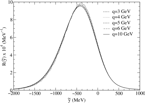
Figure 2: The response for values of $|\mathbf{q}|\geq 3$ GeV versus the scaling variable, $\tilde{y}=\nu-|\mathbf{q}|$.

In Fig. 3 we show the response at various values of $|\mathbf{q}|\leq 2$ GeV compared with that for $|\mathbf{q}|=10$ GeV, to study the approach to scaling. At small $|\mathbf{q}|$ the scattering is dominated by resonances, and the first inelastic peak is due to the lowest excited state with $n=1$ and $\ell=1$, 335 MeV above the ground state. In our toy model, the elastic scattering occurs at $\nu=0$ or $\tilde{y}=-|\mathbf{q}|$, since our hadron is heavy. This elastic scattering contribution is omitted from Fig. 3.

For $\tilde{y}\sim 0$, i.e. for small $\xi$, the response approximately scales at relatively small values of $|\mathbf{q}|$, comparable to $\sigma^{1/4}$. As $|\mathbf{q}|$ increases, the range over which scaling occurs is extended to more negative values of $\tilde{y}$, i.e. to larger values of $\xi$. The contribution of each resonance shifts to lower $\tilde{y}$ and decreases in magnitude following the $R(|\mathbf{q}|\rightarrow\infty,\tilde{y})$. This behavior is seen in the experimental data on the proton and deuteron Keppel and interpreted as evidence for quark-hadron duality. Thus the toy model seems to describe some of the observed properties of the DIS response of nucleons. It exhibits $\tilde{y}$ or equivalently $\xi$ scaling at large $|\mathbf{q}|$ as observed BPS00 , and an approach to $\xi$ scaling similar to that seen in recent experiments.

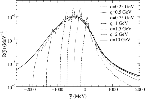
Figure 3: The approach to scaling of the response for values of $|\mathbf{q}|\leq 2$ GeV and $|\mathbf{q}|=10$ GeV versus the scaling variable, $\tilde{y}=\nu-|\mathbf{q}|$.

3.1 Particle number sum rule

In general the particle number sum rule in MBT is obtained by integrating the response at large $|\mathbf{q}|$ over all $\nu>0$:

$$\int_{0}^{\infty}R(\mathbf{q},\nu)d\nu = \sum_{I}\langle 0|\sum_{i}e^{-i\mathbf{q}\cdot\mathbf{r}_{i}}|I\rangle\langle I|\sum_{j}e^{i\mathbf{q}\cdot\mathbf{r}_{j}}|0\rangle$$ (7)

$$= \sum_{i,j}\langle 0|e^{i\mathbf{q}\cdot(\mathbf{r}_{j}-\mathbf{r}_{i})}|0\rangle.$$

When $\mathbf{q}$ is large only the $i=j$ terms in the above sum contribute, and therefore the integral gives the number of particles in the system. In contrast the sums of the response in the parton model are obtained by integrating the response over $\xi>0$ at fixed $Q^{2}$. These sums will fulfill the particle number sum rule only if the response in the timelike region is zero. As mentioned earlier, the response of a collection of noninteracting particles lies in the spacelike region. Interaction effects, however, can shift a part of the strength to the timelike region. Evidence for shifts caused by interactions is discussed in Ref. BPS00 .

Returning to the “toy” model the $R(|\mathbf{q}|,\nu)$, and therefore the $f(\tilde{y})$ extend into the timelike ($\tilde{y}>0$) region. The sum-rule given by Eq.(6), counts the number of particles in the target. It is necessary to integrate over the timelike region to fulfill this sum rule. About 10% of the sum is in that region independent of $\sqrt{\sigma}$. The response expressed as $R(Q^{2},\xi)$ also scales at large $Q^{2}$ where $|\mathbf{q}|$ is necessarily large. It becomes a function of $\xi$ alone. However, the integral:

$$\int_{0}^{\infty}R(Q^{2}\rightarrow\infty,\xi)d\xi=\int_{0}^{|\mathbf{q}|}R(|\mathbf{q}|\rightarrow\infty,\nu)d\nu\lesssim 0.9,$$ (8)

because the contribution of the timelike region is omitted. Here we have defined $\xi=|\mathbf{q}|-\nu$ without the conventional $1/M$ scale [Eq.(3)].

4 Final state interaction effects

We study the effects of the FSI of the struck particle on the response. Analytic calculations of the width of the response are presented for a general spherically symmetric potential and numerical results for a linear confining potential are given. These indicate that the FSI increase the width of the response beyond that predicted by PWIA. The analytic calculations also consider the nonrelativistic problem, in which $\mathbf{q}$ is large compared to all the momenta in the target, but smaller than the constituent mass $m$. The main differences between the nonrelativistic and the relativistic response are that the former peaks at $\nu=|\mathbf{q}|^{2}/2m$ and has a width proportional to $|\mathbf{q}|$, while the latter peaks at $\nu\sim|\mathbf{q}|$, and has a constant width in the scaling limit.

4.1 Moments of the response

In the case of a single confined particle, the state of the system after the probe has struck the target is

$$|X\rangle=e^{i\mathbf{q}\cdot\mathbf{r}}|0\rangle,$$ (9)

where $|0\rangle$ denotes the ground state of the particle. The state $|X\rangle$ is not an eigenstate of the Hamiltonian and therefore has a distribution in energy. It has a unit norm, $\langle X|X\rangle=\langle 0|e^{-i\mathbf{q}\cdot\mathbf{r}}e^{i\mathbf{q}\cdot\mathbf{r}}|0\rangle=1$. The total strength of the response, given by the static structure function

$$S(|\mathbf{q}|)=\int_{0}^{\infty}d\nu\,R(|\mathbf{q}|,\nu),$$ (10)

is therefore unity. In many-body systems $S(|\mathbf{q}|)$ is not necessarily equal to one. Subsequent formulas pertain to the general case and show factors of $S(|\mathbf{q}|)$ explicitly.

The mean excitation energy of the state $|X\rangle$ is given by the first moment of the response:

$$\overline{\nu}(|\mathbf{q}|)=\frac{1}{S(|\mathbf{q}|)}\langle X|H-E_{0}|X\rangle=\frac{1}{S(|\mathbf{q}|)}\int_{0}^{\infty}d\nu\,\nu\,R(|\mathbf{q}|,\nu).$$ (11)

The width of the distribution in energy is characterized by the second moment of the energy about the mean:

$$\Delta^{2}(|\mathbf{q}|)=\frac{1}{S(|\mathbf{q}|)}\langle X|\left(H-\frac{\langle X|H|X\rangle}{S(|\mathbf{q}|)}\right)^{\!2}|X\rangle.$$ (12)

Substitution of the Eq.(9) into the formulas for the first three moments of the response give the following results:

$$\overline{\nu}(|\mathbf{q}|) = |\mathbf{q}|+\langle V\rangle_{0}-E_{0}$$ (13)

$$+ \frac{1}{3|\mathbf{q}|}\langle k^{2}\rangle_{0}+\mathcal{O}\left(\frac{1}{|\mathbf{q}|^{3}}\right);$$

$$\Delta^{2}(|\mathbf{q}|) = \frac{1}{3}\langle k^{2}\rangle_{0}+\langle V^{2}\rangle_{0}-\langle V\rangle_{0}^{2}$$ (14)

$$+ \frac{2}{3|\mathbf{q}|}\left(\langle k^{2}V\rangle_{0}-\langle k^{2}\rangle_{0}\langle V\rangle_{0}\right)+\mathcal{O}\left(\frac{1}{|\mathbf{q}|^{2}}\right).$$

Here $\mathcal{O}\left(\frac{1}{|\mathbf{q}|^{n}}\right)$ denotes the neglected terms of that and higher order and the angle brackets with subscript ‘0’ indicate averaging with respect to the ground state. Thus $\overline{\nu}(|\mathbf{q}|)=|\mathbf{q}|-\langle T\rangle_{0}$ in the limit $|\mathbf{q}|\rightarrow\infty$, where $T=\sqrt{|\mathbf{p}|^{2}}$ is the kinetic energy. The requirement that $\overline{\nu}(|\mathbf{q}|)-|\mathbf{q}|$ becomes constant is naturally satisfied in this limit. These expression demonstrates that the average energy and width of the exact response is independent of $|\mathbf{q}|$ in the limit $|\mathbf{q}|\rightarrow\infty$ as necessary for $\tilde{y}$ scaling. It also shows that the width has a kinematic contribution dependent upon the target momentum distribution, and an additional interaction contribution.

As mentioned, the PWIA assumes that a constituent of momentum $\mathbf{k}$, after being struck by the probe, may be described by a plane wave with momentum $\mathbf{k+q}$ in an assumed average potential chosen to give the exact $\overline{\nu}$ of Eq.(13). From the PWIA response we calculate

$$\Delta^{2}_{PWIA}=\frac{1}{3}\langle k^{2}\rangle_{0}+\mathcal{O}\left(\frac{1}{|\mathbf{q}|^{2}}\right)$$ (15)

contains only the first term of the exact result [Eq.(14)] due to the target momentum distribution. The second term, $\langle V^{2}\rangle_{0}-\langle V\rangle_{0}^{2}$ of Eq.(14) represents the FSI contribution neglected in the PWIA. It does not vanish in the $|\mathbf{q}|\rightarrow\infty$ limit for relativistic kinematics.

In the non-relativistic case, $H_{NR}=\frac{|\mathbf{p}|^{2}}{2m}+V(r)$, the exact $\overline{\nu}$ is given by:

$$\overline{\nu}_{NR}=\frac{1}{2m}|\mathbf{q}|^{2}\ .$$ (16)

For the width of the NR-PWIA response we obtain:

$$\Delta^{2}_{NR-PWIA}(|\mathbf{q}|) = |\mathbf{q}|^{2}\frac{\langle k^{2}\rangle_{0}}{3m^{2}}$$ (17)

$$+ \frac{1}{4m^{2}}\left(\langle k^{4}\rangle_{0}-\langle k^{2}\rangle_{0}^{2}\right).$$

Note that in Eqs.(16) and (17) we have not taken the $|\mathbf{q}|\rightarrow\infty$ limit.

The width of the exact NR response is:

$$\Delta^{2}_{NR}(|\mathbf{q}|) = \Delta^{2}_{NR-PWIA}+\frac{1}{m}\left(\langle Vk^{2}\rangle_{0}-\langle V\rangle_{0}\langle k^{2}\rangle_{0}\right)$$ (18)

$$+ \langle V^{2}\rangle_{0}-\langle V\rangle_{0}^{2}\ .$$

It differs from $\Delta_{NR-PWIA}$ in terms of order $1/|\mathbf{q}|$ which can be neglected in the scaling limit. Thus, in contrast to the relativistic case, the FSI do not increase the width of the NR-PWIA response at large $|\mathbf{q}|$.

Finally we consider the on-shell approximation (OSA) in which the energy of the struck constituent is that of a free relativistic particle before and after the interaction with probe, as assumed in the quark-parton model. The response in OSA depends only on the momentum distribution of target constituents and obeys $\tilde{y}$ scaling. The average excitation in OSA is

$$\overline{\nu}_{OSA}=|\mathbf{q}|-\langle T\rangle_{0}+\frac{1}{3|\mathbf{q}|}\langle k^{2}\rangle_{0}+\mathcal{O}\left(\frac{1}{|\mathbf{q}|^{3}}\right),$$ (19)

and the width is given by:

$$\Delta^{2}_{OSA}=\frac{1}{3}\langle k^{2}\rangle_{0}+\langle k^{2}\rangle_{0}-\langle T\rangle_{0}^{2}+\mathcal{O}\left(\frac{1}{|\mathbf{q}|}\right).$$ (20)

The exact value of $\overline{\nu}$ [Eq.(13)] is reproduced by the OSA for any potential. However, the $\Delta^{2}_{OSA}$ has $\langle k^{2}\rangle_{0}-\langle T\rangle_{0}^{2}$ in place of the $\langle V^{2}\rangle_{0}-\langle V\rangle_{0}^{2}$ in the leading term of the exact $\Delta^{2}$ [Eq.(14)]. For a massless particle in a linear confining potential, i.e. for the Hamiltonian of Eq.(5), $\langle T\rangle_{0}=\langle V\rangle_{0}$, and $\langle k^{2}\rangle_{0}=\langle V^{2}\rangle_{0}$. Therefore for this particular Hamiltonian the OSA reproduces the exact value of $\Delta$; but the shape is wrong.

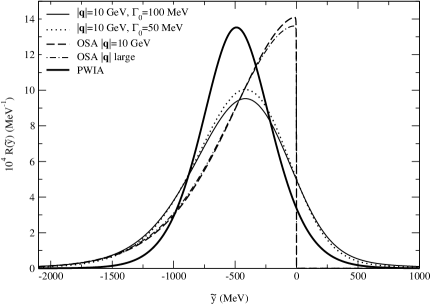
Figure 4: The response versus $\tilde{y}$ calculated exactly for $\Gamma_{0}=100$ MeV (thin solid curve) and $\Gamma_{0}=50$ MeV (dotted curve). The response in OSA are shown for $|\mathbf{q}|=10$ GeV (dashed) and $|\mathbf{q}|\rightarrow\infty$ (dot-dashed). The PWIA response for $|\mathbf{q}|=10$ GeV and $|\mathbf{q}|\rightarrow\infty$ lie on essentially the same (thick solid) curve.

4.2 Numerical results

We first compare the response functions for $|\mathbf{q}|=10$ GeV before comparing their moments. In Ref. Paris01 it has been shown that the scaling limit is obtained for such values of $|\mathbf{q}|$. The exact response, Eq.(2), is a sequence of $\delta$ functions at $\nu=E_{I}-E_{0}$. In order to obtain a smooth response we assume decay widths $\Gamma_{0}$ for all the excited states. Note that the energies of the states $|I\rangle$ that contribute to the response at $|\mathbf{q}|=10$ GeV are large, therefore their decay widths are not affected by the energy dependent terms assumed in Ref. Paris01 . The response including decay widths is given by:

$$R(\mathbf{q},\nu)=\sum_{I}|\langle I|e^{i\mathbf{q}\cdot\mathbf{r}}|0\rangle|^{2}\left(\frac{\Gamma_{0}}{2\pi}\right)\frac{1}{(E_{I}-E_{0}-\nu)^{2}+\Gamma_{0}^{2}/4}\ .$$ (21)

The responses obtained with $\Gamma_{0}=100$ and 50 MeV are shown in Fig. 4, along with the PWIA and OSA responses for $|\mathbf{q}|=10$ GeV and for $|\mathbf{q}|\rightarrow\infty$. The difference between the exact responses for $\Gamma_{0}=100$ and 50 MeV are much smaller than those between the exact and the approximate.

We note that the shape of the PWIA response is qualitatively similar to that of the exact, however, its width is too small. This is a direct consequence of the neglect of interaction terms in $\Delta$ [Eq.(14)] as discussed in the last section. The width $\Delta$ of the response is 409 MeV, while the $\Delta_{PWIA}=326$ MeV.

The OSA results in the discontinuous curves shown in Fig. 4. They are discontinuous at the lightline ($|\mathbf{q}|=\nu$) because the response of free particles is limited to the spacelike region $\nu<|\mathbf{q}|$. The discontinuity at $\tilde{y}=0$ is in clear conflict with the exact response which is continuous across the lightline and is non-zero in the timelike ($\tilde{y}>0$) region. Therefore the OSA appears to be unsatisfactory even though for the special case of a linear potential it has the exact values of $S(|\mathbf{q}|)$, $\overline{\nu}(|\mathbf{q}|)$ and $\Delta(|\mathbf{q}|)$.

References

- (1) R. K. Ellis, W. J. Stirling, and B. R. Webber, QCD and Collider Physics (Cambridge University Press, Cambridge, 1996), pg. 108.
- (2) G. Altarelli and G. Parisi, Nuc. Phys. B 126, 298 (1977).
- (3) J. D. Bjorken, in 7th Conference on the Intersections of Particle and Nuclear Physics (AIP Press, Quebec City, Quebec, Canada, 2000), hep-th/0008048.
- (4) B. Frois and I. Sick, Modern topics in electron scattering (World Scientific, Singapore, 1991).
- (5) R. N. Silver and P. E. Sokol, Momentum Distributions (Plenum Press, New York, 1989).
- (6) O. Benhar et al., Phys. Rev. C 44, 2328 (1991).
- (7) O. Benhar and V. R. Pandharipande, Phys. Rev. C 47, 2218 (1993).
- (8) S. J. Brodsky et al., Phys. Rev. D 65, 114025 (2002).
- (9) O. Benhar, V. R. Pandharipande, and I. Sick, Phys. Lett. B489, 131 (2000).
- (10) O. Nachtmann, Nucl. Phys. B 63, 237 (1973).
- (11) R. L. Jaffe, Lectures presented at the 1985 Los Alamos School on Quark Nuclear Physics, 1985.
- (12) N. Isgur, S. Jeschonnek, W. Melnitchouk, and J. W. Van Orden, Phys. Rev. D 64, 054005 (2001).
- (13) I. Niculescu et al., Phys. Rev. Lett. 85, 1182 (2000).
- (14) M. W. Paris and V. R. Pandharipande, Phys. Lett. B514, 361 (2001).