Nuclear structure near the neutron dripline: lattice HFB
calculations with high-energy continuum coupling

Abstract

We have developed a new Hartree-Fock-Bogoliubov (HFB) code which has been specifically designed to study ground state properties of nuclei near the neutron and proton drip lines. The unique feature of our code is that it takes into account the strong coupling to high-energy continuum states, up to an equivalent single-particle energy of 60 MeV. We solve the HFB equations for deformed, axially symmetric even-even nuclei in coordinate space on a 2-D lattice with Basis-Spline methods. For the p-h channel, the Skyrme (SLy4) effective N-N interaction is utilized, and for the p-p and h-h channel we use a delta interaction. We present results for binding energies, deformations, normal densities and pairing densities, Fermi levels, and pairing gaps. In particular, we will discuss neutron-rich isotopes of oxygen (${}^{22}O$) and tin (${}^{150}Sn$).

I Introduction

One of the fundamental questions of nuclear structure physics is: what are the limits of nuclear stability? How many neutrons or protons can we add to a given nucleus before it becomes unstable against spontaneous neutron or proton emission? If one connects the isotopes with zero neutron separation energy, $S_{n}=0$, in the nuclear chart one obtains the neutron dripline. Similarly, the proton dripline is defined by the condition $S_{p}=0$. Another limit to stability is the superheavy element region around $Z=124-126$ and $N=184$ which is formed by a delicate balance between strong Coulomb repulsion and additional binding due to closed shells. The nuclear chart shows less than 300 stable nuclear isotopes, and about 1700 additional isotopes have been synthesized and studied in accelerator experiments. Nuclei in between the proton and neutron driplines are unstable against $\beta$-decay. Nuclei outside the driplines decay by spontaneous neutron emission or proton radioactivity. The neutron-rich side, in particular, exhibits thousands of nuclear isotopes still to be explored (‘terra incognita’).

Some of these exotic nuclei can be studied with existing first-generation Radioactive Ion Beam Facilities (e.g. HRIBF at Oak Ridge, NSCL at Michigan State University, GANIL in France, GSI in Germany, and RIKEN in Japan). Several countries are planning to construct new ‘second generation’ RIB facilities, in particular for the exploration of neutron rich isotopes. In the United States, the DOE/NSF Long Range Plan for Nuclear Physics, published in April 2002, gives the highest priority for new construction to RIA (Rare Isotope Accelerator). RIA is a bold new concept in exotic beam facilities in that it combines both of the known rare isotope production techniques: the ISOL method (thick-target spallation) and high-energy projectile fragmentation.

Theories predict profound differences between the known isotopes near stability and the exotic nuclei at the driplines ISOL97 ; RIA1 : for n-rich nuclei, as the Fermi level approaches the particle continuum at $E=0$ (see Fig. 1) weakly bound states couple strongly to the continuum states giving rise to neutron halos and neutron skins. Theories also expect large pairing correlations and new collective modes (e.g. ‘pigmy resonance’), a weakening of the spin-orbit force leading to a quenching of the shell gaps, and perhaps new magic numbers.

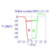
Figure 1: One-body ‘mean field’ potential for protons and neutrons. Left: for a nucleus near the stability line. Right: for a nucleus near the neutron dripline. The Fermi levels for protons and neutrons are indicated by horizontal lines.

Furthermore, RIA will allow us to address fundamental questions in nuclear astrophysics: more than half of all elements heavier than iron are thought to be produced in supernovae explosions by the rapid neutron capture process (r-process). The r-process path contains many exotic neutron-rich nuclei which can only be studied with RIA. Also, the predicted neutron skins would allow us to measure the properties of pure neutron matter which is of great interest for the study of neutron stars.

These experimental developments as well as recent advances in computational physics have sparked renewed interest in nuclear structure theory. There are several types of approaches in nuclear structure theory RIA1 : for the lightest nuclei, ab-initio calculations (Green’s function Monte Carlo, no-core shell model) based on the bare N-N interaction are possible NB97 . Medium-mass nuclei up to $A\sim 60$ may be treated in the large-scale shell model approach KDL97 . For heavier nuclei one utilizes either nonrelativistic DF84 ; DN96 or relativistic PV97 ; ND96 mean field theories.

II HFB theory in coordinate space: deformed nuclei on a 2-D lattice

An accurate treatment of the pairing interaction is essential for exotic nuclei DF84 ; DN96 . As we move away from the valley of stability, surprisingly little is known about the pairing force: for example, what is its density dependence? Neutron-rich nuclei are expected to be highly superfluid due to continuum excitation of neutron ‘Cooper pairs’. These large pairing correlations near the driplines can no longer be described by a small residual interaction. It becomes necessary to treat the mean field and the pairing field in a single self-consistent theory, known as the Hartree-Fock-Bogoliubov theory (HFB). Near the neutron dripline, the Fermi energy approaches $E=0$ and the outermost nucleons are weakly bound (which implies a large spatial extent); they are strongly coupled to the particle continuum at $E>0$. These features represent major challenges for the numerical solution.

Most HFB calculations to date are carried out in a truncated discrete harmonic ocillator basis, see e.g. RS80 ; PS90 ; CB92 ; ER93 ; SD00 .

This approach is quite appropriate for nuclei in the vicinity of the stability line. However, farther from stability, the continuum states become important and coordinate-based representations have numerous advantages: for example, the well-known ‘French code’ uses a truncated 3-D Hartree-Fock basis TH96 which consists of both localized states and discretized continuum states; however, in this approach one can only include continuum states up to about $5$ MeV of excitation energy. For nuclei in the vicinity of the driplines, continuum states with an equivalent single-particle energy of up to 60 MeV must be taken into account. One-dimensional calculations for spherical nuclei have been carried out in coordinate space for many years DF84 ; DN96 , but only recently has our Vanderbilt group succeeded in generalizing this approach to the important case of deformed axially symmetric nuclei (HFB on a 2-D lattice) OU01 ; TOU02a ; TOU02b . We utilize a novel computational technique, a Basis-Spline representation of wavefunctions and operators, which allows us to accurately describe high-energy continuum states in two space dimensions $(z,r)$.

The many-body Hamiltonian in occupation number representation has the form

$$\hat{H}=\sum_{i,j}<i|\ t\ |j>\ \hat{c}_{i}^{\dagger}\ \hat{c}_{j}+\frac{1}{2}\sum_{i,j,k,l}<ij|\ v^{(2)}\ |kl>\ \hat{c}_{i}^{\dagger}\ \hat{c}_{j}^{\dagger}\ \hat{c}_{l}\ \hat{c}_{k}+\frac{1}{6}\sum_{i,j,k,l,m,n}<ijk|\ v^{(3)}\ |lmn>\ \hat{c}_{i}^{\dagger}\ \hat{c}_{j}^{\dagger}\ \hat{c}_{k}^{\dagger}\ \hat{c}_{n}\ \hat{c}_{m}\ \hat{c}_{l}\ .$$ (1)

The general linear transformation from particle operators $\hat{c},\hat{c}^{\dagger}$ to quasiparticle operators $\hat{\beta},\hat{\beta}^{\dagger}$ take the form RS80 :

$$\left(\begin{array}[]{c}\hat{\beta}\\ \hat{\beta}^{\dagger}\end{array}\right)=\left(\begin{array}[]{cc}U^{\dagger}&V^{\dagger}\\ V^{T}&U^{T}\end{array}\right)\left(\begin{array}[]{c}\hat{c}\\ \hat{c}^{\dagger}\end{array}\right)\ .$$ (2)

The HFB approximate ground state of the many-body system is defined as a vacuum with respect to quasiparticles

$$\hat{\beta}_{k}\ |\Phi_{0}>\ =\ 0\ .$$ (3)

The HFB ground state energy including the constraint on the particle number $N$ is given by

$$E({\mathcal{R}})=<\Phi_{0}|\hat{H}-\lambda\hat{N}|\Phi_{0}>$$ (4)

where the Lagrange multiplier $\lambda$ is the Fermi energy of the system. The equations of motion are derived from the variational principle

$$\delta|_{\mathcal{R}}\ [E({\mathcal{R}})-{\rm{tr}}\ \Lambda({\mathcal{R}}^{2}-{\mathcal{R}})]=0\ ,$$ (5)

where $\mathcal{R}$ represents the generalized density matrix.

II.1 Quasiparticle wave functions and densities

In practice, it is to convenient to transform the standard HFB equations into a coordinate space representation and solve the resulting differential equations on a lattice. For this purpose, one defines two types of quasiparticle wavefunctions $\phi_{1}$ and $\phi_{2}$

$$\phi_{1}^{*}(E_{\alpha},{\bf r}\sigma q)\ =\ \sum_{i}U_{i\alpha}\ (2\sigma)\ \phi_{i}({\bf r}-\sigma q),\ \ \ \ \ \ \phi_{2}(E_{\alpha},{\bf r}\sigma q)\ =\ \sum_{i}V_{i\alpha}^{*}\ \phi_{i}({\bf r}\sigma q)\ .$$ (6)

The basis wavefunctions $\phi_{i}$ depend on the position vector ${\bf r}$, the spin projection $\sigma=\pm\frac{1}{2}$, and the isospin projection $q$ ($q=+\frac{1}{2}$ corresponds to protons and $q=-\frac{1}{2}$ to neutrons).

From these wavefunctions we obtain the following expressions for the normal density $\rho_{q}({\bf r})$ and the pairing density $\tilde{\rho}_{q}({\bf r})$

$$\rho_{q}({\bf r})=\sum_{\sigma}\sum_{\alpha}\phi_{2,\alpha}({\bf r}\sigma q)\ \phi_{2,\alpha}^{*}({\bf r}\sigma q),\ \ \ \ \ \ \tilde{\rho_{q}}({\bf r})=-\sum_{\sigma}\sum_{\alpha}\phi_{2,\alpha}({\bf r}\sigma q)\ \phi_{1,\alpha}^{*}({\bf r}\sigma q)\ .$$ (7)

The quasiparticle energy $E_{\alpha}$ is denoted by index $\alpha$ for simplicity. In principle, the sums go over all the energy states, but in practice a cutoff is introduced (see later). The physical interpretation of $\tilde{\rho_{q}}$ has been discussed in DN96 : the quantity $[\tilde{\rho_{q}}({\bf r})\ \Delta V/2]^{2}$ gives the probability to find a correlated pair of nucleons with opposite spin projection in the volume element $\Delta V$. The kinetic energy density $\tau_{q}({\bf r})$ is found to be

$$\tau_{q}({\bf r})=\sum_{\sigma}\sum_{\alpha}|\nabla\ \phi_{2,\alpha}({\bf r}\sigma q)|^{2}\ .$$ (8)

II.2 Binding energy functional

In our calculations we utilize the Skyrme two-body effective N-N interaction

$$v^{(2)}_{12} = t_{0}\ (1+x_{0}\mbox{$\hat{P}$}_{\sigma})\ \delta({\bf r}_{1}-{\bf r}_{2})+\frac{1}{2}\ t_{1}\ (1+x_{1}\mbox{$\hat{P}$}_{\sigma})\ \{\delta({\bf r}_{1}-{\bf r}_{2})\mbox{$\hat{k}$}^{2})+\mbox{$\hat{k}$}^{\prime 2}\delta({\bf r}_{1}-{\bf r}_{2})\}$$ (9)

$$+ t_{2}\ (1+x_{2}\mbox{$\hat{P}$}_{\sigma})\ \mbox{$\hat{\bf k}$}^{\prime}\cdot\delta({\bf r}_{1}-{\bf r}_{2})\ \mbox{$\hat{\bf k}$}+\frac{1}{6}\ t_{3}\ (1+x_{3}\mbox{$\hat{P}$}_{\sigma})\ \rho^{\gamma}\ \delta({\bf r}_{1}-{\bf r}_{2})+i\ W_{0}\ (\mbox{$\hat{\sigma}$}_{1}+\mbox{$\hat{\sigma}$}_{2})\cdot\{\mbox{$\hat{\bf k}$}^{\prime}\times\delta({\bf r}_{1}-{\bf r}_{2})\mbox{$\hat{\bf k}$}\}\ .$$

The density-dependent term proportional to $t_{3}$ simulates the three-body N-N interaction $v^{(3)}$.

The total binding energy of the nucleus

$$E_{0}^{HFB}=\langle\Phi_{0}|H|\Phi_{0}\rangle=E_{kin}+E_{Sky}+E_{Sky,LS}+E_{Coul}+E_{pair}+E_{cm}\ .$$ (10)

consists of a kinetic energy term, various contributions from the Skyrme effective N-N interaction (including a spin-orbit term), Coulomb and pairing energy, and a center-of mass correction due to the mean-field approximation

$$E_{kin} = \int d^{3}r\frac{\hbar^{2}}{2m}\ \tau({\bf r})$$

$$E_{Sky} = \int d^{3}r\left[\frac{b_{0}}{2}\ \rho({\bf r})^{2}+b_{1}\rho({\bf r})\tau({\bf r})-\frac{b_{2}}{2}\rho({\bf r})\nabla^{2}\rho({\bf r})+\frac{b_{3}}{3}\rho({\bf r})^{\alpha+2}\right]$$

$$+ \int d^{3}r\sum_{q}\left[-\frac{b^{\prime}_{0}}{2}\rho_{q}^{2}-b^{\prime}_{1}\rho_{q}\tau_{q}+\frac{b^{\prime}_{2}}{2}\rho_{q}\nabla^{2}\rho_{q}-\frac{b^{\prime}_{3}}{3}\rho^{\alpha}\rho_{q}^{2}\right]$$

$$E_{Sky,LS} = \int d^{3}r\left[-b_{4}\rho{\bf\nabla\cdot J}-b^{\prime}_{4}\sum_{q}\rho_{q}({\bf\nabla\cdot J}_{q})\ .\right]$$ (11)

The Coulomb energy contains the direct term as well as an exchange term (in Slater approximation)

$$E_{Coul}=\frac{e^{2}}{2}\int d^{3}r\int d^{3}r^{\prime}\rho_{p}(\mbox{${\bf r}\,$})\frac{1}{|\mbox{${\bf r}\,$}-\mbox{${\bf r}\,$}^{\prime}|}\rho_{p}(\mbox{${\bf r}\,$}^{\prime})-\frac{3}{4}e^{2}\left(\frac{3}{\pi}\right)^{1/3}\int d^{3}r\left[\rho_{p}(\mbox{${\bf r}\,$})\right]^{4/3}\ .$$ (12)

II.3 Pairing interaction

In practice, one tends to use different effective N-N interactions for the p-h / h-p channels and for the p-p / h-h channels. Most pairing calculations utilize a local pairing interaction of the form

$$V_{p}({\bf r}\sigma,{\bf r}^{\prime}-\sigma^{\prime})\ =\ V_{0}\ \delta({\bf r}-{\bf r}^{\prime})\ \delta_{\sigma,\sigma^{\prime}}\ F({\bf r})\ .$$ (13)

This parameterization describes two primary pairing forces: a pure delta interaction ($F=1$) that gives rise to volume pairing, and a density dependent delta interaction (DDDI) that gives rise to surface pairing. In the latter case, one uses the following phenomenological ansatz RD99 for the factor $F$

$$F({\bf r})\ =\ 1-\left(\frac{\rho({\bf r})}{\rho_{0}}\right)^{\gamma}$$ (14)

where $\rho({\bf r})$ is the mass density.

The pairing contribution to the nuclear binding energy is then

$$E_{pair}=\frac{V_{0}}{4}\int d^{3}r\sum_{q}\tilde{\rho}_{q}^{\ 2}({\bf r})F({\bf r})\ .$$ (15)

An important related quantity is the average pairing gap for protons and neutrons which can be calculated from the general expression given in DF84 ; DN96

$$<\Delta_{q}>\ =\ -\frac{1}{2}\ \frac{V_{0}}{N_{q}}\int d^{3}r\ \tilde{\rho_{q}}({\bf r})\ \rho_{q}({\bf r})\ F({\bf r})\ .$$ (16)

where $N_{q}$ denotes the number of protons or neutrons. Note that the pairing gap is a positive quantity because $V_{0}<0$.

II.4 HFB equations and mean fields in coordinate space

For certain types of effective interactions (e.g. Skyrme mean field and pairing delta-interactions) the particle Hamiltonian $h$ and the pairing Hamiltonian $\tilde{h}$ are diagonal in isospin space and local in position space, resulting in the following HFB equations with a 4x4 structure in spin space:

$$\left(\begin{array}[]{cc}(h^{q}-\lambda)&\tilde{h}^{q}\\ \tilde{h}^{q}&-(h^{q}-\lambda)\end{array}\right)\left(\begin{array}[]{c}\phi^{q}_{1,\alpha}\\ \phi^{q}_{2,\alpha}\end{array}\right)=E_{\alpha}\left(\begin{array}[]{c}\phi^{q}_{1,\alpha}\\ \phi^{q}_{2,\alpha}\end{array}\right)$$ (17)

with

$$h^{q}=\left(\begin{array}[]{cc}h^{q}_{\uparrow\uparrow}({\bf r})&h^{q}_{\uparrow\downarrow}({\bf r})\\ h^{q}_{\downarrow\uparrow}({\bf r})&h^{q}_{\downarrow\downarrow}({\bf r})\end{array}\right),\ \ \ \ \ \ \tilde{h}^{q}=\left(\begin{array}[]{cc}\tilde{h}^{q}_{\uparrow\uparrow}({\bf r})&\tilde{h}^{q}_{\uparrow\downarrow}({\bf r})\\ \tilde{h}^{q}_{\downarrow\uparrow}({\bf r})&\tilde{h}^{q}_{\downarrow\downarrow}({\bf r})\end{array}\right)\ \ .$$ (18)

The HFB equations have a mathematical structure that is similar to the Dirac equation: the spectrum of quasiparticle energies $E$ is unbounded from above and below. The spectrum is discrete for $|E|<-\lambda$ and continuous for $|E|>-\lambda$. This is illustrated in Fig. 2.

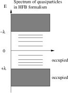
Figure 2: Computational challenge in solving the HFB equations in coordinate space: the quasiparticle energy spectrum is unbounded from above and below.

As explained in RS80 , it is forbidden to choose positive and negative quasiparticle energies at the same time, otherwise it is impossible to satisfy the anticommutation relations for $\hat{\beta}_{\alpha},\hat{\beta}_{\alpha}^{\dagger}$. For even-even nuclei it is customary to solve the HFB equations with a positive quasiparticle energy spectrum $+E_{\alpha}$ and consider all negative energy states as occupied in the HFB ground state.

The HFB mean field Hamiltonian has the same structure as the binding energy functional

$$h_{q}=-{\bf\nabla\cdot}\frac{\hbar^{2}}{2m_{q}^{*}({\bf r})}{\bf\nabla}+U_{q}({\bf r})+U_{q,LS}({\bf r})+U_{Coul}({\bf r})\cdot\delta_{q,p}\ .$$ (19)

The coordinate - dependent effective mass arises from the densities

$$\frac{\hbar^{2}}{2m_{q}^{*}({\bf r})}=\frac{\hbar^{2}}{2m_{q}}\ +\ b_{1}\ \rho({\bf r})\ -\ b^{\prime}_{1}\ \rho_{q}({\bf r})\ .$$ (20)

Detailed expressions for the Skyrme mean fields and the Coulomb term are given in reference TOU02b . The DDDI interaction generates the following pairing mean field for the two isospin orientations $q=\pm\frac{1}{2}$

$$\tilde{h}_{q}({\bf r})\ =\ \frac{1}{2}\ V_{0}\tilde{\rho_{q}}({\bf r})F({\bf r})\ .$$ (21)

III 2-D Reduction for Axially Symmetric Systems

For simplicity, we assume that the HFB quasiparticle Hamiltonian is invariant under rotations ${\hat{R}}_{z}$ around the z-axis, i.e. $[{\mathcal{H}},{\hat{R}}_{z}]=0$. Due to the axial symmetry of the problem, it is advantageous to introduce cylindrical coordinates $(\phi,r,z)$. It is possible to construct simultaneous eigenfunctions of the generalized Hamiltonian ${\mathcal{H}}$ and the z-component of the angular momentum, ${\hat{j}}_{z}$ with quantum numbers $\Omega=\pm\frac{1}{2},\pm\frac{3}{2},\pm\frac{5}{2},...$ corresponding to each $nth$ energy state. The simultaneous quasiparticle eigenfunctions take the form

$$\psi_{n,\Omega,q}(\phi,r,z)=\left(\begin{array}[]{c}\phi^{(1)}_{n,\Omega,q}(\phi,r,z)\\ \phi^{(2)}_{n,\Omega,q}(\phi,r,z)\\ \end{array}\right)=\frac{1}{\sqrt{2\pi}}\left(\begin{array}[]{c}e^{i(\Omega-\frac{1}{2})\phi}\ \phi^{(1)}_{n,\Omega,q}(r,z,\uparrow)\\ e^{i(\Omega+\frac{1}{2})\phi}\ \phi^{(1)}_{n,\Omega,q}(r,z,\downarrow)\\ e^{i(\Omega-\frac{1}{2})\phi}\ \phi^{(2)}_{n,\Omega,q}(r,z,\uparrow)\\ e^{i(\Omega+\frac{1}{2})\phi}\ \phi^{(2)}_{n,\Omega,q}(r,z,\downarrow)\end{array}\right)\ .$$ (28)

We introduce the following useful notation

$$U^{(1,2)}_{n\Omega q}(r,z)=\phi^{(1,2)}_{n,\Omega,q}(r,z,\uparrow)\ ,$$ (29)

$$L^{(1,2)}_{n\Omega q}(r,z)=\phi^{(1,2)}_{n,\Omega,q}(r,z,\downarrow)\ .$$ (30)

For axially symmetric systems, it is possible to eliminate the dependence on the angle $\phi$, resulting in the reduced 2-D problem in cylindrical coordinates TOU02b :

$$\left(\begin{array}[]{cc}(h^{\prime q}-\lambda)&\tilde{h}^{\prime q}\\ \tilde{h}^{\prime q}&-(h^{\prime q}-\lambda)\end{array}\right)\left(\begin{array}[]{c}\phi^{(1)}_{n,\Omega,q}\\ \phi^{(2)}_{n,\Omega,q}\end{array}\right)=E_{n,\Omega,q}\left(\begin{array}[]{c}\phi^{(1)}_{n,\Omega,q}\\ \phi^{(2)}_{n,\Omega,q}\end{array}\right)$$ (31)

with

$$\left(\begin{array}[]{c}\phi^{(1)}_{n,\Omega,q}\\ \phi^{(2)}_{n,\Omega,q}\\ \end{array}\right) = \left(\begin{array}[]{c}U^{(1)}_{n,\Omega,q}(r,z)\\ L^{(1)}_{n,\Omega,q}(r,z)\\ U^{(2)}_{n,\Omega,q}(r,z)\\ L^{(2)}_{n,\Omega,q}(r,z)\end{array}\right)\ .$$ (38)

Here, quantities $\tilde{h^{\prime}}$, $h^{\prime}$, $U$ and $L$ are all functions of $(r,z)$ only. This is the main mathematical structure that we implement in computational calculations. For a given angular momentum projection quantum number $\Omega$, we solve the eigenvalue problem to obtain energy eigenvalues $E_{n,\Omega,q}$ and eigenvectors $\psi_{n,\Omega,q}$ for the corresponding HFB quasiparticle states.

From the definitions of the normal density and pairing density we find the corresponding expressions in axial symmetry:

$$\rho_{q}(r,z) = \frac{1}{2\pi}\left(2\sum_{\Omega>0}^{\Omega_{max}}\right)\times\sum_{E_{n}>0}^{E_{max}}\left[|U^{(2)}_{n\Omega q}(r,z)|^{2}+|L^{(2)}_{n\Omega q}(r,z)|^{2}\right]$$ (39)

$$\tilde{\rho}_{q}(r,z) = -\frac{1}{2\pi}\left(2\sum_{\Omega>0}^{\Omega_{max}}\right)\times\sum_{E_{n}>0}^{E_{max}}\left[U^{(2)}_{n\Omega q}(r,z)U^{(1)*}_{n\Omega q}(r,z)+L^{(2)}_{n\Omega q}(r,z)L^{(1)*}_{n\Omega q}(r,z)\right]\ .$$ (40)

IV Lattice representation of spinor wavefunctions and Hamiltonian

We solve the HFB eigenvalue problem by direct diagonalization on a two-dimensional grid $(r_{\alpha},z_{\beta})$, where $\alpha=1,...,N_{r}$ and $\beta=1,...,N_{z}$. The four components of the spinor wavefunction are represented on the two-dimensional lattice by an expansion in basis-spline functions $B_{i}(x)$ evaluated at the lattice support points. Further details about the basis-spline technique are given in Ref. Uma91 ; WO95 .

For the lattice representation of the Hamiltonian, we use a hybrid method K96 ; KO96 ; Obe99 in which derivative operators are constructed using the Galerkin method; this amounts to a global error reduction. Local potentials are represented by the basis-spline collocation method (local error reduction). The lattice representation transforms the differential operator equation into a matrix form

$$\sum_{\nu=1}^{N}{\cal{H}}_{\mu}^{\ \nu}\psi^{\Omega}_{\nu}=E^{\Omega}_{\mu}\psi^{\Omega}_{\mu}\ \ \ (\mu=1,...,N)\ ,$$ (41)

The calculations use as a starting point the result of a HF+BCS previous calculation, which makes HFB converge substantially faster. Since the problem is self-consistent we use an iterative method for the solution. At every iteration the full HFB Hamiltonian is diagonalized. Due to the axial symmetry in the intrinsic frame, the diagonalization is performed separately for each value of the angular momentum projection quantum number $\Omega$ and for the two isospin projections $q=\pm\frac{1}{2}$. Typically 20-30 iterations are sufficient for convergence at the level of one part in $10^{5}$ for the total binding energy.

Note that in this lattice approach, the number of quasiparticle states is determined by the dimensionality of the discrete HFB Hamiltonian which is $N=(4N_{r}N_{z})^{2}$.

V Numerical results

In the following we discuss some numerical results obtained with our new HFB-2D code. First we present calculations for a light stable nucleus, ${}^{22}_{10}$Ne. This nucleus was chosen because it has a large prolate g.s. quadrupole deformation. The calculation has been performed with the Skyrme SLy4 interaction in the p-h channel and a pure delta pairing interaction (strength $V_{0}=-173MeVfm^{3}$). For the pairing forces of zero range employed here, one needs to introduce an energy cut-off. In all of our calculations, we use a cut-off energy $E_{max}=60$ MeV in the equivalent s.p. energy spectrum, the same value utilized by Dobaczewski et al. DN96 in his spherical 1-D calculations.

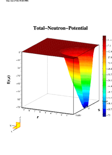
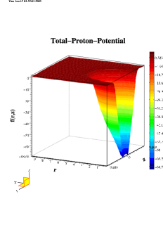
Figure 3: ²²Ne mean field potential for neutrons and protons

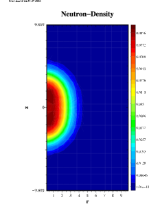
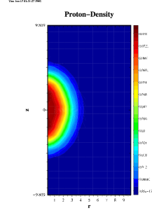
Figure 4: Neutron and proton density distribution for the strongly deformed nucleus ²²Ne

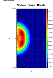
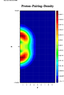
Figure 5: Neutron and proton pairing density distribution for ²²Ne

Fig. 3 shows the mean field potential $U_{q}({\bf r})$ for neutrons and protons. Both mean fields are fairly similar, except that there is an additional Coulomb contribution for the protons. In Fig. 4 we depict contour plots of the normal density for neutrons and protons. The large prolate quadrupole deformation is clearly visible in the density distributions. Fig. 5 shows the pairing density for neutrons and protons. The square of the pairing density describes the probability of finding a correlated nucleon pair with opposite spin directions at position ${\bf r}$ DN96 . Because this is a stable isotope, the pairing turns out to be relatively weak. The shell structure of this light nucleus causes significant differences in the neutron- vs. proton pairing.

We now present results for the n-rich isotope ${}^{22}O$ which is close to the experimentally confirmed RIA1 dripline nucleus ${}^{24}O$. Because this nucleus turns out to be spherical in our 2-D calculations, we can compare our results to the 1-D spherical code of Dobaczewski DF84 and to the 2-D oscillator basis expansion method of Stoitsov et al. SD00 . Table 1 shows several observables for this nucleus: the total binding energy, Fermi levels, pairing gaps and the r.m.s. radius. Overall, the results of the axially symmetric code of the present work agree with the other two in all observables.

Table 1: Comparison of several HFB calculations for ${}^{22}O$. In all cases, the mean field is calculated with the SLY4 interaction, and the pairing force is a pure delta interaction (strength $V_{0}=-218.5MeVfm^{3}$) corresponding to volume pairing. The axially symmetric calculations (2D) of this work used a box size $R=10fm$ with maximum $j_{z}=\frac{9}{2}$. The spherical calculation of Ref. Dpriv was made with $R=25fm$ and a $j_{max}=\frac{21}{2}$.

	1-D DN96 ; Dpriv	2-D (THO)SD00 ; Stpriv	2-D (this work)
total binding energy (MeV)	-164.60	-164.52	-164.64
Fermi level, neutrons (MeV)	-5.26	-5.27	-5.29
Fermi level, protons (MeV)	-18.88	-18.85	-18.08
pairing gap, neutrons (MeV)	1.42	1.41	1.36
pairing gap, protons (MeV)	0.0	0.0	0.0
r.m.s. radius (fm)	2.92	2.92	2.92

We now turn our attention to the heavy neutron rich isotope ${}^{150}Sn$ $(Z=50,N=100)$ which has twice as many neutrons as protons. In some phenomenological models, it is already close to the 2-neutron dripline. Fig. 6 shows contour plots of the normal density for neutrons and protons. Because of the magic proton number and due to strong pairing, the nuclear shape turns out to be spherical in our 2-D HFB code. In Fig. 7 we depict a cut of these densities in radial direction which clearly exhibits the ‘neutron skin’ already seen in the 1-D calculations of Ref. DN96 . The neutron skin represents a region of pure neutron matter which will allow us to the study the properties of neutrons stars in future laboratory experiments at RIA.

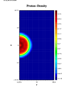
Figure 6: Neutron and proton density distribution for ${}^{150}_{\ 50}$Sn, a nucleus near the two-neutron dripline

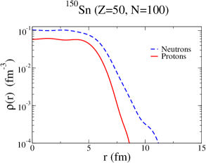
Figure 7: Cut in radial direction of the neutron and proton density in ${}^{150}_{\ 50}$Sn. The neutron skin is clearly visible.

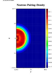
Figure 8: Neutron and proton pairing density distribution for ${}^{150}_{\ 50}$Sn. Because of the magic proton number $Z=50$ the proton pairing density is exactly zero.

In Table 2 we compare again our 2-D calculations with the 1-D radial results of Ref. DN96 . In the 2-D calculations an approximately $3000\times 3000$ matrix was diagonalized for each $j_{z}$ and isospin value, and for each major HFB iteration. The full calculation required about 20 HFB iterations. All observables agree quite well. The neutron Fermi level is less than $1MeV$ in this case which demonstrates clearly the proximity of ${}^{150}Sn$ to the two-neutron drip line.

Table 2: Comparison of 1-D and 2-D calculations for ${}^{150}Sn$. In both cases, the mean field is calculated with the SLY4 interaction, and the pairing force is a pure delta interaction (strength $V_{0}=-170MeVfm^{3}$) corresponding to volume pairing. The 1-D calculations used a box size $R=30$ with $j_{max}$ of $\frac{21}{2}$. Calculations with our axially symmetric HFB 2-D code were made using a box size $R=20fm$ with maximum $j_{z}=\frac{13}{2}$.

	1-D DN96 ; Dpriv	2-D (this work)
total binding energy (MeV)	-1129	-1130
Fermi level, neutrons (MeV)	-0.96	-0.94
Fermi level, protons (MeV)	-17.54	-17.34
pairing gap, neutrons (MeV)	1.02	0.97
pairing gap, protons (MeV)	0.00	0.00
r.m.s. radius (fm)	5.126	5.132

VI Summary and Conclusions

Our goal for the near future is to investigate several isotope chains, in particular deformed nuclei, and to calculate observables which are important for the physics near the drip lines, i.e. binding energies, neutron and proton separation energies, pairing gaps, particle densities and pairing densities, rms radii, and electric or magnetic moments. We plan to utilize a variety of Skyrme parameterizations for the mean field, and both volume and surface pairing forces. As more data from existing RIB facilities become available, it is likely that it will become necessary to develop new effective N-N interactions to describe these exotic nuclei. Furthermore, our 2-D HFB code results may be used as input into coordinate-space based QRPA calculations to investigate collective excited states (surface vibrations and giant resonances).

We will also study alternative numerical techniques to speed up our 2-D HFB code, in particular damping methods which we have utilized successfully in solving the Dirac equation WO95 . Provided that the damping method can be successfully implemented in 2-D, we will attempt to solve the 3-D HFB problem in Cartesian coordinates. This will certainly be very difficult, but it is worth trying: in the 1996 DOE/NSAC Long Range Plan, unrestricted HFB theory on the lattice has been described as a computational Grand Challenge project in nuclear physics.

- (1) ‘Scientific Opportunities with an Advanced ISOL Facility’, Panel Report (Nov. 1997), ORNL.
- (2) ‘RIA Physics White Paper’, RIA 2000 Workshop, Raleigh-Durham, NC (July 2000), distributed by NSCL, Michigan State University.
- (3) P. Navratil, B.R. Barrett and W.E. Ormand, Phys. Rev. C 56, 2542 (1997).
- (4) D. Dean, presentation at this conference; S.E. Koonin, D.J. Dean, and K. Langanke, Phys. Rep. 1, 278 (1997).
- (5) J. Dobaczewski, H. Flocard, and J. Treiner, Nucl. Phys. A422, 103 (1984).
- (6) J. Dobaczewski, W. Nazarewicz, T.R. Werner, J.F. Berger, C.R. Chinn, and J. Dechargé, Phys. Rev. C53, 2809 (1996).
- (7) W. Pöschl, D. Vretenar, G.A. Lalazissis and P. Ring, Phys. Rev. Lett. 79, 3841 (1997).
- (8) W. Nazarewicz, J. Dobaczewski, T.R. Werner, J.A. Maruhn, P.-G. Reinhard, K.Rutz, C.R. Chinn, A.S. Umar, M.R. Strayer, Phys. Rev. C 53, 740 (1996).
- (9) P. Ring and P. Schuck, ”The Nuclear Many-Body Problem”, (Springer Verlag, New York, 1980).
- (10) A. Petrovici, K.W. Schmid, F. Grümmer, and A. Faessler, Nucl. Phys. A517, 108 (1990).
- (11) C.R. Chinn, J.-F. Berger, D. Gogny and M.S. Weiss, Phys. Rev. C45, 1700 (1992).
- (12) J.L. Egido and L.M. Robledo, Phys. Rev. Lett. 70, 2876 (1993).
- (13) M.V. Stoitsov, J. Dobaczewski, P. Ring, and S. Pittel, Phys. Rev. C 61, 034311 (2000).
- (14) J. Terasaki, P.-H. Heenen, H. Flocard, and P. Bonche, Nucl. Phys. A600, 371 (1996).
- (15) V.E. Oberacker, A.S. Umar, J. Chen, and E. Teran, Proc. International Conference on Physics with Radioactive Ion Beams (ISOL’01), Oak Ridge, TN, March 2001, to be published, 2001; nucl-th/0103038
- (16) HFB calculations near the drip lines, E. Teran, V.E. Oberacker, and A.S. Umar, to be published in Heavy Ion Physics, 2002; nucl-th/0110059.
- (17) E. Teran, V.E. Oberacker and A.S. Umar, ‘Axially symmetric Hartree-Fock-Bogoliubov Calculations for Nuclei Near the Drip-Lines’, nucl-th/0205042
- (18) A.S. Umar, J. Wu, M.R. Strayer, and C.Bottcher, J. Comp. Phys. 93, 426 (1991).
- (19) J.C. Wells, V.E. Oberacker, M.R. Strayer and A.S. Umar, Int. J. Mod. Phys. C6, 143 (1995).
- (20) D.R. Kegley, Ph.D. thesis, Vanderbilt University (1996).
- (21) D.R. Kegley, V.E. Oberacker, M.R. Strayer, A.S. Umar, and J.C. Wells, J. Comp. Phys. 128, 197 (1996).
- (22) V.E. Oberacker and A.S. Umar, in “Perspectives in Nuclear Physics” (ed. J.H. Hamilton, H.K. Carter and R.B. Piercey), World Scientific Publ. Co. (1999), p. 255-266.
- (23) P.-G. Reinhard, D.J. Dean, W. Nazarewicz, J. Dobaczewski, J. A. Maruhn, and M.R. Strayer, Phys. Rev. C 60, 014316 (1999).
- (24) E. Chabanat, P. Bonche, P. Haensel, J. Meyer, and R. Schaeffer, Nucl. Phys. A635, 231 (1998); Nucl. Phys. A643, 441 (1998).
- (25) J. Dobaczewski, Warsaw (private communication).
- (26) M. Stoitsov, ORNL (private communication).