Viscous Corrections to Spectra, Elliptic Flow, and HBT Radii
Abstract
I compute the first viscous correction to the thermal distribution function. With this correction, I calculate the effect of viscosity on spectra, elliptic flow, and HBT radii. Indicating the breakdown of hydrodynamics, viscous corrections become of order one for . Viscous corrections to HBT radii are particularly large and reduce the outward and longitudinal radii. This reduction is a direct consequence of the reduction in longitudinal pressure.
1 Viscous Corrections
Ideal hydrodynamics describes a wide variety of data from heavy ion collisions [1, 2]. In particular ideal hydrodynamics successfully predicted the observed elliptic flow and its dependence on mass, centrality, beam energy, and transverse momentum. Nevertheless, the hydrodynamic approach failed in several respects. First, above a transverse momentum the particle spectra deviate from hydrodynamics and approach a power law. Second, HBT radii are significantly too large compared to ideal hydrodynamics [3]. Considering the partial success of ideal hydrodynamics, viscous corrections may provide a natural explanation for these failures.
For an ideal Bjorken expansion, the entropy per unit space-time rapidity is conserved. For a viscous Bjorken expansion the entropy per unit rapidity increases as a function of proper time [4]
| (1) |
where is the shear viscosity. In this equation and below we have neglected the bulk viscosity. For hydrodynamics to be valid, the entropy produced over the time scale of the expansion (to wit, ) must be small compared to the the total entropy (). This leads to the requirement that
| (2) |
where we have defined the sound attenuation length as . Perturbative estimates of the shear viscosity in the plasma give . Below we take , assuming that non-perturbative effects shorten equilibration times.
Viscosity modifies the thermal distribution function. This modification influences the observed particle spectrum and HBT correlations. The formal procedure for determining the viscous correction to the thermal distribution function is described in references [5, 6]. However, the basic form of the viscous correction can be intuited without calculation. First write , where is the equilibrium thermal distribution function and is the first viscous correction. is linearly proportional to the spatial gradients in the system. Spatial gradients which have no time derivatives in the rest frame and are therefore formed with the differential operator . For a baryon free fluid, these gradients are , , and , where . can be eliminated in favor of the other two spatial gradients using the condition that and the ideal equations of motion. leads ultimately to a bulk viscosity and will be neglected in what follows. Finally, leads to a shear viscosity. If is restricted to be a polynomial of degree less than two, then the functional form of the viscous correction is completely determined,
| (3) |
For a Boltzmann gas this is the form of the viscous correction adopted in this work. For Bose and Fermi gasses the ideal distribution function in Eq. 3 is replaced with [6].
The coefficient is directly related to the sound attenuation length. Indeed, using the distribution function in Eq. 3 to determine the stress energy tensor, yields a relationship between the shear viscosity and the coefficient ,
| (4) |
For a Boltzmann gas, Eq. 4 yields .
The thermal distribution function is now completely determined. In the next section this correction is used to calculate corrections to the observables used in heavy ion collisions.
2 Corrections to Spectra, Elliptic Flow, HBT Radii
To quantify the effect of viscous corrections on spectra and HBT radii, I generalize the blast wave model. In the blast wave model used here, the matter undergoes a boost invariant Bjorken expansion and decouples at a proper time of at a temperature of . The matter is distributed uniformly up to a radius of , with velocity profile up to a maximum velocity 111In contrast to common practice is linearly rising: . The blast wave model with these parameters closely models the output of a full hydrodynamic simulation [1, 2] and gives a reasonable fit of the data.
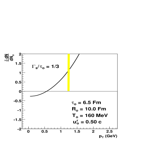
the ratio of the correction compared to the ideal spectrum, .
To understand this figure qualitatively, consider a Bjorken expansion of infinitely large nuclei. The longitudinal pressure is reduced [4], . Because the shear tensor is traceless, the transverse pressure is increased, . Thus, the matter distribution is pushed out to larger by the shear in the longitudinal direction. More mathematically, the ratio of the corrected spectrum to the uncorrected spectrum is given by,
| (7) |
For large we find, . Eq. 7 reproduces the shape and dependence of the full viscous blast wave calculation shown in Fig. 2.
Viscous corrections become of order one when the of the particle approaches GeV. This signals the breakdown of the hydrodynamic approach. In fact, ideal hydrodynamics generally fails to reproduce the single particle spectra above of 1.5 GeV. Viscosity provides a ready explanation for this breakdown.
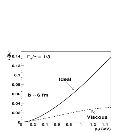
In non-central collisions elliptic flow is calculated using the spectrum indicated in Eq. 5. In non-central collisions, the matter is assumed to have a cylindrical distribution but the flow velocity has an elliptic component, . For non-central collisions the parameters are: and . As illustrated in Fig. 2, viscosity reduces elliptic flow by a factor of three.
Next consider viscous corrections to HBT radii. The HBT radii are calculated with the method of variances. First the ideal radii parameters are displayed in Fig. 4. The results
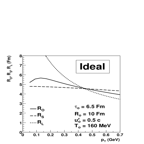
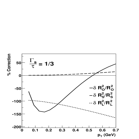
are typical of the blast wave parametrization. Next the viscous correction to the blast wave results are illustrated in Fig. 4.
Viscous corrections to and are large and negative. This may be understood qualitatively by again considering a simple Bjorken expansion of infinite nuclei. The longitudinal pressure is reduced, . Therefore the distribution () is narrower. However, by boost invariance the single particle distribution () is a function of , which yields the relation,
| (8) |
The distribution () at mid rapidity is therefore
narrower because the longitudinal pressure is reduced. This implies
that decreases due to the
viscous longitudinal
expansion. In summary, viscosity provides a simple explanation for
the very large radii predicted by ideal hydrodynamics.
Acknowledgments: This work was supported by DE-AC02-98CH10886.
References
- [1] D. Teaney, J. Lauret, and E.V. Shuryak, Phys. Rev. Lett. 86, 4783 (2001); D. Teaney, J. Lauret, and E.V. Shuryak, nucl-th/0110037.
- [2] P.F. Kolb, P.Huovinen, U. Heinz, H. Heiselberg, Phys. Lett. B 500, 232 (2001); P. Huovinen, P.F. Kolb, U. Heinz, H. Heiselberg, Phys. Lett. B 503, 58 (2001).
- [3] S. Soff, S. A. Bass, Adrian Dumitru, Phys. Rev. Lett. 86, 3981 (2001).
- [4] P. Danielewicz, M. Gyulassy, Phys. Rev. D 31, 53-62 (1985).
- [5] S. de Groot, W. van Leeuven, Ch. van Veert, Relativistic Kinetic Theory (North-Holland, 1980).
- [6] Peter Arnold, Guy D. Moore, Laurence G. Yaffe, JHEP 0011, 001 (2000).