Analytical approach to electromagnetic processes in loosely bound nuclei: application to $\@@nuc{8}{B}$

Abstract

In this paper we develop an analytical model in order to study electromagnetic processes involving loosely bound neutron–rich and proton–rich nuclei. We construct a model wave function, to describe loosely bound few–body systems, having the correct behaviour both at large and small distances. The continuum states are approximated by regular Coulomb functions. As a test case we consider the two–body Coulomb dissociation of $\@@nuc{8}{B}$ and, the inverse, radiative capture reaction. The difference between using a pure two–body model and the results obtained when incorporating many–body effects, is investigated. We conclude that the interpretation of experimental data is highly model dependent and stress the importance of measuring few–body channels.

, and Electromagnetic processes such as radiative capture, photo–dissociation and Coulomb dissociation have always been, and still remain, an excellent tool to investigate nuclear structure. Unfortunately, for radioactive nuclei the radiative capture experiments are very difficult and studies of photo–dissociation are virtually impossible. However, with the advent of radioactive beam facilities, nuclear structure of dripline nuclei can be studied using Coulomb dissociation on heavy targets. The Coulomb breakup of these nuclei is of interest also in nuclear astrophysics, since it can be related to the corresponding radiative capture process at astrophysical energies [1]. In this paper, we will present an analytical model for Coulomb dissociation (and consequently for radiative capture) of loosely bound dripline nuclei (see also our recent conference contribution [2]). We want to stress that our approach will be general in the sense that both neutron–rich, and proton–rich systems can be studied. The possibility to study reactions analytically is very appealing since it often allows a deeper physical understanding of the process. For some cases such studies are not only possible but might even give results that are directly comparable to experimental data and more advanced, numerical calculations. In particular, this is the case for electromagnetic transitions between a loosely bound nuclear state and a pure Coulomb continuum. “Loosely bound” implies that the nucleus will exhibit a large degree of clusterization. We will consider the case of two clusters, but will also discuss the three–cluster channel (see also similar approaches for one–neutron [3, 4, 5] and two–neutron [6, 7, 8] halo nuclei). After a general description of our model we will exemplify it with an application to $\@@nuc{8}{B}$. Our main focus will be the nuclear structure effects, and we will utilize the advanced three–body model of Grigorenko et al. [9], while the Coulomb dissociation is considered only to first order. As it was shown recently [10, 11], higher order effects should not be significant at beam energies higher than around 70 MeV/$A$.

Our starting point for calculating electromagnetic cross sections will be the $\mathrm{E}\lambda$ strength function for a transition from an initial state to a final, continuum state with energy $E$

$$\frac{\mathrm{d}B(\mathrm{E}\lambda)}{\mathrm{d}E}=\frac{1}{2J_{i}+1}\sum_{f}\int\d\tau_{f}\left|\langle f||\mathcal{M}(\mathrm{E}\lambda)||i\rangle\right|^{2}\delta\left(E_{f}-E\right),$$ (1)

where $\mathrm{d}\tau_{f}$ is the phase space element for final states, $\mathcal{M}(\mathrm{E}\lambda)$ is the electric multipole operator and $|i\rangle$, $|f\rangle$ are the initial and final states in the center of mass subsystem.

We will consider loosely bound systems of two clusters $(c+x)$ and, in particular, we will study transitions to the low–energy continuum in which excitations are manifested as relative motion between the clusters $E=\hbar^{2}k^{2}/2\mu_{cx}$, where $\mu_{cx}$ is the reduced mass of the system. Introducing the intercluster distance, $r$, the corresponding cluster $\mathrm{E}\lambda$ operator (operating only on the relative motion of clusters) is

$$\mathcal{M}(\mathrm{E}\lambda,\mu)=eZ(\lambda)r^{\lambda}Y_{\lambda\mu}(\hat{r}),$$ (2)

with the effective multipole charge $Z(\lambda)=\mu_{cx}^{\lambda}(Z_{x}/m_{x}^{\lambda}+(-1)^{\lambda}Z_{c}/m_{c}^{\lambda})$.

The strength function is the key to study several reactions. The photo–dissociation $(A+\gamma\rightarrow c+x)$ cross section is given by

$$\sigma_{\gamma}^{\mathrm{E}\lambda}(E_{\gamma})=\frac{(2\pi)^{3}(\lambda+1)}{\lambda[(2\lambda+1)!!]^{2}}\left(\frac{E_{\gamma}}{\hbar c}\right)^{2\lambda-1}\frac{\mathrm{d}B(\mathrm{E}\lambda)}{\mathrm{d}E},$$ (3)

where the photon energy, $E_{\gamma}=E+E_{0}$, is larger than the binding energy, $E_{0}$. The inverse radiative capture reaction can be studied using detailed balance

$$\sigma_{\mathrm{rc}}^{\mathrm{E}\lambda}(E)=\left(\frac{E_{\gamma}}{\hbar ck}\right)^{2}\frac{2(2J_{A}+1)}{(2J_{c}+1)(2J_{x}+1)}\sigma_{\gamma}^{\mathrm{E}\lambda}(E_{\gamma}),$$ (4)

where $J_{i}$ is the spin of particle $i$. Using first order perturbation theory, and the method of virtual quanta [12, 13], the energy spectrum for Coulomb dissociation on a high–$Z$ target can be written as a sum over multipole, $\pi\lambda$, photo–dissociation cross sections multiplied by the corresponding spectra of virtual photons, $n_{\pi\lambda}(E_{\gamma})$,

$$\frac{\mathrm{d}\sigma_{\mathrm{C}}}{\mathrm{d}E}=\sum_{\mathrm{E}\lambda}\frac{n_{\mathrm{E}\lambda}(E_{\gamma})}{E_{\gamma}}\sigma_{\gamma}^{\mathrm{E}\lambda}(E_{\gamma})+\sum_{\mathrm{M}\lambda}\frac{n_{\mathrm{M}\lambda}(E_{\gamma})}{E_{\gamma}}\sigma_{\gamma}^{\mathrm{M}\lambda}(E_{\gamma}).$$ (5)

Note that since M$\lambda$ transitions are usually [13] strongly suppressed we will not consider them in this work. In order to study all these reactions analytically we will propose a model function to describe the (loosely) bound state of a two–body system. We will only be interested in direct transitions to a “clean” continuum, i.e., with all nuclear phase shifts equal to zero. Thus, the final state, with angular momentum $l_{f}$ between the clusters, will be described by a regular Coulomb function

$$\phi_{l_{f}}(k,r) =\sqrt{\frac{2}{\pi}}\frac{1}{k}i^{l_{f}}e^{i\sigma_{l_{f}}}F_{l_{f}}(k,r),\qquad\mathrm{where}$$ (6)

$$F_{l_{f}}(k,r) =C_{l_{f}}(k)e^{ikr}(kr)^{l_{f}+1}{}_{1}F_{1}(l_{f}+1+i\eta(k);2l_{f}+2;-2ikr),$$ (7)

and $\sigma_{l_{f}}$ is the Coulomb phase, $\eta(k)=Z_{c}Z_{x}e^{2}\mu_{cx}/\hbar^{2}k$ is the Sommerfeld parameter, $C_{l_{f}}(k)=2^{l_{f}}e^{-\pi\eta(k)/2}|\Gamma(l_{f}+1+i\eta(k))|/(2l_{f}+1)!$, and ${}_{1}F_{1}(a;b;z)$ is the confluent hypergeometric function [14].

The reduced matrix element introduced in the definition of the strength function, Eq. (1), contains a radial integral. With our approximation for the continuum state this integral takes the form

$$I_{l_{f}}(k)=\int_{0}^{\infty}\mathrm{d}re^{-ikr}r^{l_{f}+1}{}_{1}F_{1}(l_{f}+1-i\eta(k);2l_{f}+2;2ikr)r^{\lambda}\phi_{b}(r).$$ (8)

Here, $\phi_{b}(r)$ is the two–body, relative motion wave function (WF) describing the initial state. For large $r$, and with angular momentum $l_{i}$ between the clusters, this radial function should be proportional to the Whittaker function $W_{-\eta_{0},l_{i}+1/2}(2\kappa_{0}r)$ (see Ref. [14]), where $\eta_{0}=Z_{c}Z_{x}e^{2}\mu_{cx}/\hbar^{2}\kappa_{0}$ and $E_{0}=\hbar^{2}\kappa_{0}^{2}/2\mu_{cx}$ is the binding energy.

In most studies on loosely bound systems, the Whittaker function has been used to describe the bound state for all $r$. However, this approximation is only motivated if the transition matrix element is dominated by contributions from very large $r$. This should be the case for reactions at very small energies. For real experimental energies ($E\gtrsim 100$ keV), the WF of the bound state should be constructed in a more realistic way. Therefore we will introduce a model function that describes the bound state $c+x$ WF accurately for all distances. This is done by considering the behavior at small and large $r$. We have already pointed out the the WF should be described by a Whittaker function at large $r$. Furthermore, for a two–body system, consisting of point–like particles, it should behave as $r^{l_{i}+1}$ as $r\rightarrow 0$. Both asymptotics are fulfilled using the following model function

$$\phi_{b,\tilde{\gamma}}^{\mathrm{``exact^{\prime\prime}}}(r)=\frac{1}{\sqrt{N_{\tilde{\gamma}}}}W_{-\eta_{0},l_{i}+1/2}(2\kappa_{0}r)\left(1-e^{-\kappa_{1}r}\right)^{2l_{i}+1},$$ (9)

where $N_{\tilde{\gamma}}$ is the normalization constant and $\tilde{\gamma}$ denotes the parameters $\left\{\kappa_{0},\kappa_{1},\eta_{0}\right\}$. The parameters $\kappa_{0}$ and $\eta_{0}$ are defined by the binding energy, charges and masses, while $\kappa_{1}$ can be fitted to give the correct size of the system. Using this WF, and solving the integral (8) numerically, it is possible to get very good estimates for the electromagnetic reaction cross sections. As a remark we want to point out that, for a one–neutron halo nucleus ($\eta_{0}=0$), the Whittaker function will transform into a modified, spherical Bessel function: $W_{0,l_{i}+1/2}(2\kappa_{0}r)=\sqrt{2\kappa_{0}r/\pi}K_{l_{i}+1/2}(\kappa_{0}r)$. In this case, the integral (8) can be solved exactly.

However, we are searching for a completely analytical model which will also enable us to incorporate many–body effects. Our model function (9) has to be modified accordingly. First, we note that the asymptotic form of the Whittaker function as $r\rightarrow\infty$ is

$$W_{-\eta_{0},l_{i}+1/2}(2\kappa_{0}r)\sim e^{-\kappa_{0}r}r^{-\eta_{0}}\left[1+\mathcal{O}(1/r)\right].$$ (10)

Secondly, for two–body systems in which the clusters have an internal structure, the centrifugal barrier is effectively larger and the WF should behave as $r^{n}$, where $n>l_{i}+1$, as $r\rightarrow 0$.

Motivated by this, we put forward the following model function

$$\phi_{b,\gamma}(r) =\frac{1}{\sqrt{N_{\gamma}}}\frac{e^{-\kappa_{0}r}}{r^{\eta_{0}^{\prime}}}\left(1-e^{-\kappa_{1}r}\right)^{p},\qquad\mathrm{with~{}norm}$$ (11)

$$N_{\gamma} =\sum_{m=0}^{2p}\binom{2p}{m}(-1)^{m}(2\kappa_{0}+m\kappa_{1})^{2\eta_{0}^{\prime}-1}\Gamma(1-2\eta_{0}^{\prime}),$$

where $\gamma$ denotes the parameters $\left\{\kappa_{0},\kappa_{1},\eta_{0}^{\prime},p\right\}$. The parameter $\kappa_{0}$ is defined by the binding energy and effective mass. By putting $\eta_{0}^{\prime}=\eta_{0}$ we would ensure to reproduce the tail of the WF at very large $r$. However, higher order terms in Eq. (10) remain important for $r\lesssim 100$ fm. Therefore, $\eta_{0}^{\prime}$ and $\kappa_{1}$ are used as free parameters in a fit to the “exact” WF (9) in the interval of interest. In this way $\eta_{0}^{\prime}$ will be an “effective” Sommerfeld parameter while $\kappa_{1}$ will still mainly be connected with the size. Finally, the integer $p$ is fixed by the small $r$ behaviour, $r^{n}$, and will thus allow us to take many–body effects into account.

It is now possible to make the integral (8) analytically (see Ref. [15])

$$\begin{split}I_{l_{f},\gamma}(k)=\frac{1}{\sqrt{N_{\gamma}}}\sum_{m=0}^{p}\binom{p}{m}(-1)^{m}(m\kappa_{1}+\kappa_{0}+ik)^{-(l_{f}+2+\lambda-\eta_{0}^{\prime})}\Gamma(l_{f}+2+\lambda-\eta_{0}^{\prime})\\ \times{}_{2}F_{1}\left(l_{f}+2+\lambda-\eta_{0}^{\prime};l_{f}+1-i\eta(k);2l_{f}+2;\frac{2ik}{m\kappa_{1}+\kappa_{0}+ik}\right).\end{split}$$ (12)

Many-body nuclear structure can further be taken into account by considering the possibility that the bound state WF contains several different two–body components

$$\phi_{b}(r)=\sum_{i}a_{i}\phi_{b,\gamma_{i}}(r).$$ (13)

Note that pure many–body components will not contribute to two–body breakup, but will instead lead to $\sum_{i}a_{i}^{2}<1$. Note also that the threshold for two–body breakup will be higher for components where one (or both) of the clusters is excited. Therefore, we define the continuum strength function separately for each component. Finally, we arrive at an analytical formula for the strength function

$$\left.\frac{\mathrm{d}B(\mathrm{E}\lambda)}{\mathrm{d}E}\right|_{i}=\frac{e^{2}Z^{2}(\lambda)\mu_{cx}}{\hbar^{2}}\frac{2\lambda+1}{2\pi^{2}}\sum_{l_{f}}a_{i}^{2}k^{2l_{f}+1}C_{l_{f}}^{2}(k)\langle l_{i}0\lambda 0|l_{f}0\rangle^{2}|I_{l_{f},\gamma_{i}}(k)|^{2}.$$ (14)

As an example we will apply our analytical approach to the ⁸B nucleus. Our key point here will be to show the applicability of our analytical model and to demonstrate the importance of many–body nuclear structure. The interest in ⁸B stems from its key role in the production of high-energy solar neutrinos. The probability of the reaction $\@@nuc{7}{Be}$$+p\rightarrow$$\@@nuc{8}{B}$$+\gamma$ at solar energies strongly depends on the structure of $\@@nuc{8}{B}$ and, in particular, on the asymptotics of the valence proton WF. The reaction can be studied indirectly through Coulomb dissociation, using a radioactive ⁸B beam on a heavy target [16, 17, 18, 19]. We should also mention the recent progress in radiative capture measurements [20], where the cross section has been measured at energies around 200 keV with an accuracy of $\approx 15$ percent. However, in all cases theoretical models are needed to extrapolate the measured cross sections down to solar energies.

The low–lying $\@@nuc{8}{B}$ continuum can, with relatively good precision, be approximated as a pure Coulomb one. There are no negative parity states at low excitation energies [21] and the electromagnetic processes are, in all cases we are considering, dominated by $\mathrm{E}1$ transitions.

We start by treating $\@@nuc{8}{B}$ as a pure two–body ($\@@nuc{7}{Be}+p$) system with binding energy $E_{0}=137$ keV and relative orbital momentum $l_{i}=1$. The single free parameter, $\kappa_{1}$, in our “exact” model function (9) is then fitted to an rms intercluster distance of $r_{\mathrm{rms}}=4.57$ fm (extracted from Ref. [9]). In order to get analytical results, we then introduce the model function (11). With $p=2l_{i}+1=3$ and $\kappa_{0}$ fixed from the binding energy, the remaining parameters $\kappa_{1}$ and $\eta_{0}^{\prime}$ are fitted to the behavior of the “exact” model function (9), see Table 1. The resulting E1 strength function is showed as a dashed line in Fig. 1. This analytical approximation agrees, to a very high precision, with the numerical results obtained keeping the “exact” model function. The error is less than 2 % in the region of interest.

However, concerning the structure of the $\@@nuc{8}{B}$ ground state, one should keep in mind that the $\@@nuc{7}{Be}$ core is in itself a weakly bound system with an excited $1/2^{-}$ state at 429 keV. The common treatment of $\@@nuc{8}{B}$ as a two–body system is therefore highly questionable. We now want to investigate what effect the many–body structure of $\@@nuc{8}{B}$ might have on the strength function. We utilize a recent three–body calculation [9], where it was shown that, after projection on the two–body channel, there are three main components (adding up to 94 % of the total WF), and that the rest are pure three–body channels, see Table 1. For each of these two–body components we fit our parameters $\kappa_{1}$ and $\eta_{0}^{\prime}$. The binding energy, $E_{0}=137$ keV, determines $\kappa_{0}$ for the two first components and $E_{0}=566$ keV for the third, $\@@nuc{7}{Be}$ excited state, component. The best fit of the small $r$ behavior is obtained with $p=5$ which reflects the effectively larger centrifugal barrier in the three–body case. This centrifugal barrier will push the WF away from $r=0$ and will, thus, force it to become more narrow than the two–body WF. We therefore expect the distribution in momentum/energy space to be broader. This effect is clearly seen in Fig. 1 where the E1 strength function obtained using this three–body model is shown as a solid line. This difference, seen in the strength function, should be even more pronounced in the energy spectrum. From these results one can conclude that the interpretation of energy spectra is highly model dependent.

In Fig. 2(a) we compare our analytical results for Coulomb dissociation, including both E1 and E2 transitions, to the experimental data from Davids et al. [17]. This experiment is very appealing since the selection of scattering angles ($\theta_{\@@nuc{8}{B}}\leq 1.77^{\circ}$) minimizes the contribution from nuclear scattering and the relatively high beam energy (82.7 MeV/$A$) justifies the use of first order perturbation theory. Concerning the shape of the energy spectrum we have an excellent agreement between the experimental data and our results obtained using the three–body model (see thin, dotted line), while the pure two–body calculation gives a too narrow peak. As to the absolute values, the three–body model gives about 20 % larger cross section than the experimental data. In Fig. 2(b) we compare the results from our two–body model (dashed line) to the results from a potential model calculation without final state interaction, from [22] (dash–dotted). Here, the intercluster distance for both models is $r_{\mathrm{rms}}=4.23$ fm which is lower than before ($r_{\mathrm{rms}}=4.57$ fm). The lesson from this figure is twofold. Firstly, it demonstrates the sensitivity to the intercluster distance and the importance of knowing this parameter. Secondly, we note that the difference between the two–body potential model calculation and our analytical results is not so large. The results deviate mainly in the peak amplitude.

In connection to the same experimental conditions we show in Fig. 3 the fraction of the cross section that can be attributed to E1 transitions. This information is of importance when studying the inverse radiative capture reaction and, in contrast to the conclusion drawn by Davids et al. [17], we claim that although the E2 contribution increases for low relative energies, it still does not dominate. Note that including M1 transitions will give raise to a sharp dip at 640 keV.

We have also compared our results for the radiative capture reaction to the experimental data by Hammache et al. [20]. Our three–body result of $\sigma_{\mathrm{rc}}(186\mathrm{~{}keV})=16.1$ nb agrees very well with the experimental value $16.7\pm 2.1$ nb. We also find that the E2 contribution to this cross section is around 0.03 %.

In conclusion, we have performed analytical studies of electromagnetic processes for loosely bound nuclei. This has been accomplished by using model radial functions that describe two–body WFs or the two–body projections of many–body WFs, accurately for all radii, and by only studying direct transitions to/from a pure Coulomb continuum. We have examined the difference between a pure two–body model and the results obtained incorporating many–body effects. From this we concluded that the interpretation of experimental data is highly model dependent. Comparisons have also been made to experimental results on $\@@nuc{8}{B}$ Coulomb dissociation and, the inverse, radiative capture reaction. We found that our three–body results coincide with the radiative capture cross section measured by Hammache et al. [20] while our Coulomb dissociation energy spectrum is about 20 % larger than the experimental data from Davids et al. [17]. However, the shapes of the experimental and theoretical energy spectra are in excellent agreement. In contrast, our pure two–body model of $\@@nuc{8}{B}$, having the same intercluster distance $r_{\mathrm{rms}}$, does not agree with the experimental data. A final word of wisdom is that, in order to interpret these data correctly, it is very important to fix the spectroscopic factors of different two–body and many–body components. Therefore, we want to stress the usefulness of experiments where Coulomb dissociation is studied in complete kinematics. Examples of interesting channels in the $\@@nuc{8}{B}$ case is $\@@nuc{8}{B}$$\rightarrow$$\@@nuc{7}{Be}$($1/2^{-}$)$+p+\gamma$ and $\@@nuc{8}{B}$$\rightarrow$$\@@nuc{3}{He}$$+\alpha+p$. Recently, $\@@nuc{7}{Be}$ fragments and $\gamma$–rays were measured in coincidence after breakup on a light target by Cortina–Gil et al. [16] and the excited core component of the WF was clearly observed.

N. B. S. is grateful for support from the Royal Swedish Academy of Science. The support from RFBR Grants No 00–15–96590, 02–02–16174 are also acknowledged.

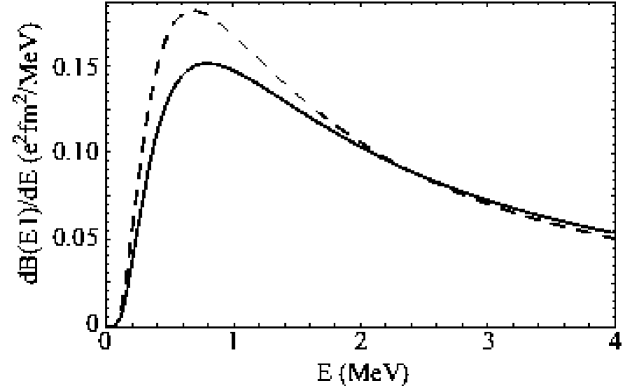
Figure 1: The E1 strength function of $\@@nuc{8}{B}$. Although the total strength is the same, the shapes are very different when treating the $\@@nuc{8}{B}$ nucleus as a two–body (dashed line) or a three–body (solid line) system. The difference is mainly due to the stronger centrifugal barrier in the three–body case forcing the WF to be narrower and thus wider in momentum/energy space. The parameters of the model WFs can be found in Table 1.

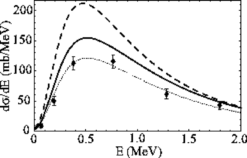
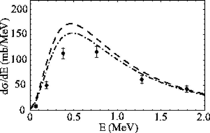
(a)

(b)

Figure 2: The $\@@nuc{8}{B}$ Coulomb dissociation energy spectrum obtained at 82.7 MeV/$A$ on Pb with $\@@nuc{8}{B}$ scattering angles $\leq 1.77^{\circ}$. The data points are from [17]. In (a) the curves show our analytical two–body (dashed line) and three–body (solid line) calculations, while the thin, dotted line is just a scaled version of the three–body result. In (b) the dash–dotted line is the cross section calculated numerically within a two–body potential model, from [22]. A comparison is made with our analytical two–body model (dashed line) having the same intercluster distance. All theoretical curves have been corrected for experimental resolution and acceptance.

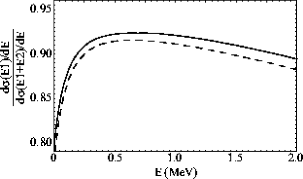
Figure 3: Fraction of the calculated cross section for the Coulomb dissociation of 82.7 MeV/$A$ $\@@nuc{8}{B}$ on Pb with scattering angles $\leq 1.77^{\circ}$ attributed to E1 transitions. The curves are two–body (dashed line) and three–body (solid line) calculations.

Table 1: Parameters of our model WFs used to describe the $\@@nuc{8}{B}$ ground state. Both models give the same intercluster distance, $r_{\mathrm{rms}}=4.57$ fm. With $E_{0}=137$ keV we get $\kappa_{0}=0.076$ fm^-1 and $\eta_{0}=1.595$. The excited core component (last row) has $E_{0}=566$ keV giving $\kappa_{0}=0.154$ fm^-1 and $\eta_{0}=0.786$. The relative orbital momentum for all components are $l_{i}=1$ while $I$ is the channel spin and $a^{2}$ is the spectroscopic factor. Note that there is no dependence on channel spin in our strength function (14).

Model WF	configuration	$I$	$a^{2}$	$p$	$\kappa_{1}$ (fm-1)	$\eta_{0}^{\prime}/\eta_{0}$
two–body	$\left[\@@nuc{7}{Be}(3/2^{-})\otimes p\right]$	2	1.00	3	0.601	0.79
	$\left[\@@nuc{7}{Be}(3/2^{-})\otimes p\right]$	2	0.65	5	0.702	0.87
	$\left[\@@nuc{7}{Be}(3/2^{-})\otimes p\right]$	1	0.13	5	0.765	0.86
three–body	$\left[\@@nuc{7}{Be}(1/2^{-})\otimes p\right]$	1	0.16	5	0.753	1.43

References

- [1] M. S. Smith and K. E. Rehm, Annu. Rev. Nucl. Part. Sci. 51, 91 (2001).
- [2] C. Forssén, V. D. Efros, N. B. Shul’gina, and M. V. Zhukov, in Nuclei in the Cosmos VII, to be published in Nucl. Phys. A.
- [3] C. A. Bertulani and G. Baur, Nucl. Phys. A 480, 615 (1988).
- [4] T. Otsuka, M. Ishihara, N. Fukunishi, T. Nakamura, and M. Yokoyama, Phys. Rev. C 49, R2289 (1994).
- [5] D. M. Kalassa and G. Baur, J. Phys. G 22, 115 (1996).
- [6] A. Pushkin, B. Jonson, and M. V. Zhukov, J. Phys. G 22, 95 (1996).
- [7] C. Forssén, V. D. Efros, and M. V. Zhukov, Nucl. Phys. A 697, 639 (2002).
- [8] C. Forssén, V. D. Efros, and M. V. Zhukov, Nucl. Phys. A 706, 48 (2002).
- [9] L. V. Grigorenko, B. V. Danilin, V. D. Efros, N. B. Shulgina, and M. V. Zhukov, Phys. Rev. C 60, 044312 (1999).
- [10] S. Typel, H. H. Wollter, and G. Baur, Nucl. Phys. A 613, 147 (1997).
- [11] P. Banerjee, G. Baur, K. Hencken, R. Shyam, and D. Trautmann, Phys. Rev. C 65, 064602(7) (2002).
- [12] A. Winther and K. Alder, Nucl. Phys. A 319, 518 (1979).
- [13] C. A. Bertulani and G. Baur, Nucl. Phys. A 442, 739 (1985).
- [14] M. Abramowitz and I. A. Stegun, editors, Handbook of Mathematical Functions, Dover Publications, Inc., New York, 1972.
- [15] I. S. Gradshteyn and I. M. Ryzhik, Table of Integrals, Series and Products, Academic Press, Inc., San Diego, second edition, 1980.
- [16] D. Cortina-Gil et al., Phys. Lett. B 529, 36 (2002).
- [17] B. Davids et al., Phys. Rev. C 63, 065806 (2001).
- [18] N. Iwasa et al., Phys. Rev. Lett. 83, 2910 (1999).
- [19] T. Kikuchi et al., Phys. Lett. B 391, 261 (1997).
- [20] F. Hammache et al., Phys. Rev. Lett. 86, 3985(4) (2001).
- [21] G. V. Gol’dberg, V. Z.and Rogatchev, V. I. Dukhanov, I. N. Serikov, and V. A. Timofeev, JETP Lett. 67, 1013 (1998).
- [22] C. A. Bertulani, Z. Phys. A 356, 293 (1996).
(a)
(b)