Effective Field Theory for Fermi Systems in a large $N$ expansion

Abstract

A system of fermions with short-range interactions at finite density is studied using the framework of effective field theory. The effective action formalism for fermions with auxiliary fields leads to a loop expansion in which particle-hole bubbles are resummed to all orders. For spin-independent interactions, the loop expansion is equivalent to a systematic expansion in $1/N$, where “$N$” is the spin-isospin degeneracy $g$. Numerical results at next-to-leading order are presented and the connection to the Bose limit of this system is elucidated.

I Introduction

Effective field theory (EFT) provides a powerful framework to study low-energy phenomena in a model-independent way by exploiting the separation of scales in physical systems Weinberg79 ; LEPAGE89 ; KAPLAN95 . Only low-energy (or long-range) degrees of freedom are included explicitly, with the short-range physics parametrized in terms of the most general local (contact) interactions. Using renormalization, the influence of high-energy states on low-energy observables is captured in a small number of constants. Thus, the EFT describes universal low-energy physics independent of detailed assumptions about the high-energy dynamics. Recent applications of EFT methods to nuclear physics have made steady progress in the two- and three-nucleon sectors EFT98 ; EFT99 ; Birareview ; BEANE99 ; Bedaque:2002mn . In this paper, we continue a complementary program to apply EFT methods to many-fermion systems, with the ultimate goal of describing nuclei and nuclear matter.

We showed the promise of using effective field theory for the nuclear many-body problem in Ref. HAMMER00 , where a dilute, uniform gas of fermions interacting via short-range interactions (which could be highly singular potentials such as hard cores) was analyzed. In general, this problem is nonperturbative in the potential, so the conventional diagrammatic treatment sums particle-particle ladder diagrams to all orders and thereby replaces the bare interaction by a $K$ matrix FETTER71 ; BISHOP73 . Each $K$ matrix is in turn replaced by an effective range expansion in momentum, and in the end one finds a perturbative expansion of the energy per particle [see Eq. (22)] in terms of the Fermi momentum $k_{\rm F}$ times the $S$-wave scattering length $a_{s}$ (and other effective range parameters in higher orders).

In contrast, the EFT approach is more direct, transparent, and systematic. The EFT automatically recasts the problem in the form of a perturbative Fermi momentum expansion. The freedom to use different regulators and renormalization schemes was exploited by choosing dimensional regularization with minimal subtraction (DR/MS), for which the dependence on dimensional scales factors cleanly into $k_{\rm F}$ dependence solely from the loop integrals and dependence on effective range parameters solely in the coefficients. This allowed power counting by simple dimensional analysis and manifested the universal nature of the low-order contributions.

Power counting refers to a procedure that identifies the contributions to a given order in an EFT expansion; this is an essential feature of the EFT approach. In the dilute case, the power counting with DR/MS is particularly simple: each diagram contributes at a single order in $k_{\rm F}$ and there are a finite number of diagrams at each order. This renormalization scheme also simplified a renormalization group analysis to identify logarithmic divergences that lead to nonanalytic (logarithmic) terms in the $k_{\rm F}$ expansion of the energy Braaten97 ; HAMMER00 .

Thus, the application of EFT methods to the dilute Fermi system exhibits a consistent organization of many-body corrections, with reliable error estimates, and insight into the analytic structure of observables. EFT provides a model-independent description of finite-density observables in terms of parameters that can be fixed from scattering in the vacuum or from a subset of finite-density properties. The universal nature of the expansion is also a key feature; any underlying potential, probed at long distance, is reproduced by the same form and the differences lie only in the low-energy constants. This perturbative analysis is directly applicable to systems of trapped atoms and provides a controlled theoretical laboratory for studying issues such as the status of occupation numbers as observables Furnstahl:2001xq or the nature of the Coester line FURNSTAHL01 .

However, bound nuclear systems and the most interesting phenomena in atomic systems require a nonperturbative EFT treatment. The most conspicuous features of nuclear interactions leading to nonperturbative physics are the large $S$-wave scattering lengths. The analysis in Ref. HAMMER00 assumes that the (spin-averaged) scattering length is of natural size (e.g., of order the range of the underlying interaction). When the scattering length is large, the expansion applies only at very small $k_{\rm F}$, and an alternative power counting is needed to extend the EFT to larger densities. This power counting, developed in Refs. vanKolck:1998bw and ksw for two-particle scattering in free space, prescribes that leading order for large $a_{s}$ must sum all diagrams with non-derivative four-fermion ($C_{0}$) vertices (although in higher orders the other vertices appear only perturbatively). For two-particle scattering, this infinite set of diagrams is easily summed as a geometric series. In three-body systems, large scattering lengths necessitate three-body input at leading order to remove regularization dependence Bedaque:1998kg ; Bedaque:1999ve . The shallowness of the deuteron and triton bound states ensures that the physics of large scattering lengths is dominant in these systems.

At finite density, the class of diagrams with $C_{0}$ vertices is much larger than in free space, since it also includes tadpoles, particle-hole rings, hole-hole rings, and so on. These diagrams are not simply summed and have not been calculated numerically. As an alternative to a direct numerical solution, we can seek additional expansions. Possibilities include geometric Steele:2000qt , strong-coupling, or large-$N$ expansions. In the present work, we investigate the most immediate extension that is nonperturbative in $k_{\rm F}a_{s}$ by adopting an effective action formalism, which is a natural framework for implementing nonperturbative resummations. As we illustrate below, the loop expansion in the auxiliary field formulation for spin-independent forces is equivalent to a systematic $1/N$ expansion, where the relevant “$N$” is the spin-isospin degeneracy $g$.

In Coleman’s classic lecture on the $1/N$ expansion, he identifies two reasons to pursue such expansions COLEMAN88 . First, they can be used to analyze model field theories so that intuition beyond perturbation theory can be developed. They provide nontrivial, but tractable examples (at least qualitatively) to build intuition about phenomena such as asymptotic freedom, dynamical symmetry breaking, dimensional transmutation, and nonperturbative confinement. We seek similar controlled insight into nonperturbative effects in nonrelativistic many-body systems. The large-$g$ expansion has a well-defined power counting that sums certain classes of diagrams to all orders to provide a systematic expansion for systems where $k_{\rm F}a_{s}$ is small (natural scattering length) but $gk_{\rm F}a_{s}/\pi$ is order unity or greater. The expansion for natural scattering length has the interesting feature that it is nonperturbative in the medium while the description of free-space scattering is perturbative. For large $a_{s}$, the expansion may not be fully systematic, but could still provide insight into the nonperturbative many-body physics.

The second reason for pursuing $1/N$ expansions is that they may be relevant to physical systems of interest. Coleman (and many others) considered quantum chromodynamics (QCD) with a large number $N_{c}$ of colors, arguing that the large $N_{c}$ world is in many ways close to the real world of $N_{c}=3$. But while $1/N$ expansions of QCD and other relativistic field theories are common Brezin:eb , they have been exploited much less widely in nonrelativistic many-fermion physics and very little in applications to nuclear systems. In fact, the principle applications have been to one-dimensional Fermi systems Calog75 ; Yoon77 . However, there have been some applications of $1/N$ expansions in relativistic approaches to nuclear systems. In Ref. TANAKA93 , e.g., the Walecka model was studied in a $1/N$ expansion by extending the $SU(2)$ isospin symmetry to $SU(N)$. To our knowledge, the present work is the first on effective action EFT and the $1/N$ expansion for nonrelativistic Fermi systems with short-range interactions in three dimensions.

In Ref. NEGELE88 , expansions in $1/g$ are discussed, but with the caveat that they are not likely relevant to nuclear systems, even though $g=4$ would seem to be large enough. This is based on the observation that with empirical nonrelativistic interactions, exchange (Fock) contributions are larger than direct (Hartree) contributions, whereas the former should be suppressed by $1/g$ relative to the latter. However, this dismissal may be premature. In a different phenomenological representation of the problem, using covariant interactions, the Hartree pieces do, in fact, dominate Furnstahl:1999ff . Furthermore, the expansion may be useful to describe part of the physics, such as if the long-distance pion physics is removed Steele:1998zc or averaged out Furnstahl:2001un . Indeed, analyses of phenomenological energy functionals fit to bulk nuclear properties suggest a robust power counting with short-distance scale $\Lambda$ roughly 600 MeV Furnstahl:2000in . At nuclear matter equilibrium densities, this would imply $k_{\rm F}/\Lambda$ is less than one, but $gk_{\rm F}/\Lambda$ is greater than one! (However, the expansion parameter may actually be $gk_{\rm F}/\Lambda\pi$, as suggested by the analysis in Sect. IV.)

An interesting special case of the $g\rightarrow\infty$ limit follows if we also take the Fermi momentum $k_{\rm F}$ to zero, with the density (which is proportional to $gk_{\rm F}^{3}$) held constant. We refer to this procedure as the “Bose limit,” because it generates the ground state of a dilute Bose system (under the assumption that the ground state evolves adiabatically from the noninteracting state). This limit was noted long ago in Refs. GENTILE40 and SHUBERT46 but was not exploited until Brandow used it in comparing fermionic (³He) and bosonic (⁴He) many-body systems BRANDOW71 . In Ref. JACKSON94 , Jackson and Wettig used the Bose limit in analyzing minimal many-body approximations and cleanly derived the leading corrections to the Bose energy (see also Ref. NEGELE88 in this connection.)

In Sect. II, we summarize the effective action formalism for fermions using an auxiliary field. In Sect. III, we review the EFT treatment of a dilute Fermi system with short-range, spin-independent interactions and then apply the effective action formalism. We carry out the loop expansion, which is seen to correspond to a $1/g$ expansion. In Sect. IV, we calculate the energy per particle explicitly to next-to-leading order (NLO) and perform a stability analysis of the ground state. The Bose limit is considered in Sect. V, and Sect. VI contains a summary of our results and conclusions, along with plans for further investigations.

II Effective action for fermions with auxiliary fields

In this section, we review the effective action formalism for fermions with auxiliary fields at zero temperature ($T=0$). We adopt the notation and spirit of the general discussion of effective actions in Ref. PESKIN95 and largely follow the specific treatment of nonrelativistic fermions by Fukuda et al. FUKUDA94 . Our discussion will be somewhat schematic in order to focus on the new aspects of the EFT treatment. Details of the renormalization of the effective action and caveats related to convergence of the path integrals, Wick rotations from Euclidean space, zero-temperature limits, and so on are well documented and can be found in the standard literature COLEMAN88 ; NEGELE88 ; PESKIN95 ; FUKUDA94 ; ITZYKSON80 ; WEINBERG96 .

Consider a system of fermions in an external potential $v(x)$ interacting via a spin-independent, local two-body interaction $U_{0}(x-y)$. (The extension to many-body forces in the context of an EFT is outlined in Appendix A.) Such a system is described by the Lagrangian

$${\cal L} = {\psi^{\dagger}_{\alpha}}(x)\left({i\partial_{t}}+\frac{\overrightarrow{\nabla}^{2}\!}{2M}+\mu+v(x)\right)\psi_{\alpha}(x)-\frac{1}{2}{\psi^{\dagger}_{\alpha}}(x){\psi^{\dagger}_{\beta}}(y)U_{0}(x-y)\psi_{\beta}(y)\psi_{\alpha}(x)\,,$$ (1)

where $\alpha,\,\beta$ are spin indices, $\mu$ is the chemical potential, and $M$ the fermion mass. We define a generating functional $Z[J]$ and an energy functional $E[J]$ via the relation (we follow the notation from Ref. PESKIN95 )

$$Z[J]=e^{-iE[J]}=\int{\cal D}{\psi^{\dagger}}{\cal D}\psi\,e^{i\int\!d^{4}x\,[{\cal L}+J(x){\psi^{\dagger}_{\alpha}}(x)\psi_{\alpha}(x)]}\,,$$ (2)

where $J(x)$ is an external source. For simplicity, normalization factors are considered to be implicit in the functional integration measure.

The strategy is first to reduce $Z[J]$ to a Gaussian integral in the fermion Grassmann fields by “integrating in” an auxiliary field HandS ; NEGELE88 . Using the identity FUKUDA94

$$1=\frac{\int{\cal D}\sigma\exp\left(\frac{i}{2}\int\!d^{4}x\int\!d^{4}y\,[\sigma(x)-{\psi^{\dagger}_{\alpha}}(x)\psi_{\alpha}(x)]U_{0}(x-y)[\sigma(y)-{\psi^{\dagger}_{\beta}}(y)\psi_{\beta}(y)]\right)}{\int{\cal D}\sigma\exp\left(\frac{i}{2}\int\!d^{4}x\int\!d^{4}y\,\sigma(x)U_{0}(x-y)\sigma(y)\right)}\,,$$ (3)

we introduce an auxiliary field $\sigma$ with bosonic quantum numbers and obtain for the generating functional with $J=0$ (i.e., the partition function)

$$Z[J]|_{J=0} = \int{\cal D}\,{\psi^{\dagger}}{\cal D}\psi\,{\cal D}\sigma\exp\bigg{[}i\int\!d^{4}x\,{\psi^{\dagger}_{\alpha}}(x)\bigg{(}{i\partial_{t}}+\frac{\overrightarrow{\nabla}^{2}\!}{2M}+\mu+v(x)\bigg{)}\psi_{\alpha}(x)$$ (4)

$$\hbox{}-{\psi^{\dagger}_{\alpha}}(x)\psi_{\alpha}(x)\int\!d^{4}z\,U_{0}(x-z)\sigma(z)+\frac{1}{2}\sigma(x)\int\!d^{4}y\,U_{0}(x-y)\sigma(y)\bigg{]}\,,$$

where the denominator of Eq. (3) has been absorbed into the normalization of $Z$. The ${\cal D}{\psi^{\dagger}}{\cal D}\psi$ path integral is now Gaussian and leads to a determinant of the operator between ${\psi^{\dagger}}$ and $\psi$, which we identify as an inverse fermion propagator:

$$G^{-1}(x,y)\,\delta_{\alpha\beta} \equiv \biggl{[}{i\partial_{t}}+\frac{\overrightarrow{\nabla}_{x}^{2}\!}{2M}+\mu+v(x)-\int\!d^{4}zU_{0}(x-z)\sigma(z)\biggr{]}\delta^{4}(x-y)\,\delta_{\alpha\beta}\ .$$ (5)

Note that this propagator still depends on the field $\sigma$ but is manifestly diagonal in the spin (or flavor) indices. We exponentiate the determinant using $\det A=\exp[{\rm Tr}\ln A]$ and reintroduce a source term, now coupled to the $\sigma$ field, to obtain

$$Z[J] = e^{-iE[J]}=\int{\cal D}\sigma\exp\bigg{(}g{\rm Tr}\ln\bigg{[}G^{-1}(x,y)\bigg{]}\bigg{)}$$ (6)

$$\hbox{}\times\exp\bigg{(}\frac{i}{2}\int\!d^{4}x\!\int\!d^{4}y\,\sigma(x)U_{0}(x-y)\sigma(y)\bigg{)}\exp\bigg{(}i\int\!d^{4}xJ(x)\sigma(x)\bigg{)}\,,$$

where the spin/flavor trace has been performed in the first term, leading to the spin/flavor degeneracy factor $g$ (e.g., for electrons or neutrons, $g=2$ and for symmetric nuclear matter, $g=4$). The remaining trace in the first line of Eq. (6) is over space-time.

We define the “classical field” $\sigma_{c}(x)$ in the presence of $J(x)$ by the ground state expectation value of $\sigma(x)$:

$$\sigma_{c}(x)\equiv\langle\Omega|\sigma(x)|\Omega\rangle_{J}=-\frac{\delta}{\delta J(x)}E[J]=-i\frac{\delta}{\delta J(x)}\ln Z[J]\,,$$ (7)

and define the effective action

$$\Gamma[\sigma_{c}]\equiv-E[J]-\int\!d^{4}x\,J(x)\sigma_{c}(x)\,,$$ (8)

in the usual way PESKIN95 . The effective action has the property

$$\frac{\delta}{\delta\sigma_{c}(x)}\Gamma[\sigma_{c}]=-J(x)\,,$$ (9)

and the solutions for $J(x)=0$ represent the stable quantum states PESKIN95 . At the minimum $\sigma_{c}^{0}$ (with $J(x)=0$) of a uniform system, the energy density ${\cal E}$ of the ground state is related to the effective action by

$$\left.\Gamma[\sigma_{c}^{0}]\right|_{J=0}=-VT{\cal E}\,,$$ (10)

where $VT$ is the space-time volume of the system. More generally, at finite density we must examine spatially dependent $\sigma_{c}^{0}$ to find the absolute ground state.

To evaluate $\Gamma[\sigma_{c}]$ in a loop expansion, we write $\sigma=\sigma_{c}+\eta$ and expand Eq. (6) in quantum fluctuations $\eta$ around the classical field $\sigma_{c}$. Once again we seek a Gaussian path integral, this time in terms of $\eta$, while using a source coupled to $\eta$ to treat the residual $\eta$-dependent terms perturbatively (by removing them from the path integral in favor of functional derivatives with respect to the source). The expansion, integration, and subsequent Legendre transformation are standard and we simply quote the result for the effective action from Refs. FUKUDA94 ; PESKIN95 :

$$\Gamma[\sigma_{c}] = \frac{g}{i}\,{\rm Tr}\ln[G_{H}^{-1}(x,y)]+\frac{1}{2}\int\!d^{4}x\int\!d^{4}y\,\sigma_{c}(x)U_{0}(x-y)\sigma_{c}(y)$$ (11)

$$+\frac{i}{2}{\rm Tr}\ln\left[D_{\sigma}^{-1}(x,y)\right]+\int\!d^{4}x\,\delta{\cal L}[\sigma_{c}]+\mbox{(connected 1PI-diagrams)}\,.$$

In Eq. (11), we have introduced the inverse Hartree propagator (which depends on $\sigma_{c}$ but not $\eta$)

$$G_{H}^{-1}(x,y) \equiv \biggl{[}{i\partial_{t}}+\frac{\overrightarrow{\nabla}_{x}^{2}\!}{2M}+\mu+v(x)-\int\!d^{4}zU_{0}(x-z)\sigma_{c}(z)\biggr{]}\delta^{4}(x-y)\ ,$$ (12)

and the inverse $\sigma$ propagator

$$D_{\sigma}^{-1}(x,y)\equiv-iU_{0}(x-y)+g\int\!d^{4}z_{1}\int\!d^{4}z_{2}\,G_{H}(z_{1},z_{2})U_{0}(z_{2}-x)G_{H}(z_{2},z_{1})U_{0}(z_{1}-y)\,,$$ (13)

which originates with the part of the exponential in $Z[J]$ that is quadratic in $\eta$ after expanding. The counterterm Lagrangian $\delta{\cal L}$ has been included in Eq. (11) for completeness; however, with the regularization/renormalization procedure applied here (DR/MS), we will not need it explicitly PESKIN95 .

The two propagators are obtained by solving the equations

$$\int\!d^{4}z\,G_{H}^{-1}(x,z)G_{H}(z,y) = \delta^{4}(x-y)\,,$$

$$\int\!d^{4}z\,D_{\sigma}^{-1}(x,z)D_{\sigma}(z,y) = \delta^{4}(x-y)\,,$$ (14)

with appropriate boundary conditions for $G_{H}$ and $D_{\sigma}$ (discussed below). The “connected 1PI-diagrams” in Eq. (11) are built from the propagator $D_{\sigma}$ for the $\sigma$ field and the vertices

$$V_{m}(x_{1},..,x_{m})=\int\!d^{4}y_{1}...\int\!d^{4}y_{m}\,G_{H}(y_{m},y_{1})\,U_{0}(y_{1}-x_{1})..G_{H}(y_{m-1},y_{m})\,U_{0}(y_{m}-x_{m})\,,$$ (15)

where $m=3,\ldots,\infty$. We follow Ref. PESKIN95 and use the freedom of a counterterm $\delta J$ to ensure that $\sigma_{c}$ is the same to all orders in the expansion (i.e., $\langle\eta\rangle=0$), which simplifies the bookkeeping. As a consequence, all diagrams that are 1-particle reducible with respect to the $\sigma$ propagator are cancelled and only 1-particle irreducible diagrams have to be included in calculations of the effective action. In the next section, we show how this expansion, when applied to the lowest-order EFT potential, is an expansion in inverse powers of $g$.

III Dilute Fermi systems with short-range interactions

In this section, we apply the effective action formalism to the Fermi gas with short-range, spin-independent interactions. We calculate the effective action to one loop explicitly and demonstrate that the loop expansion of the effective action corresponds to a large $N$ expansion.

III.1 Short-range EFT and Low-density Expansion

We consider a general local Lagrangian for a nonrelativistic fermion field that is invariant under Galilean, parity, and time-reversal transformations:

$${\cal L} = \psi^{\dagger}\biggl{[}i\partial_{t}+\frac{\overrightarrow{\nabla}^{\,2}}{2M}\biggr{]}\psi-\frac{C_{0}}{2}(\psi^{\dagger}\psi)^{2}+\frac{C_{2}}{16}\Bigl{[}(\psi\psi)^{\dagger}(\psi\tensor{\nabla}^{2}\psi)+\mbox{ h.c.}\Bigr{]}$$ (16)

$$\hbox{}+\frac{C_{2}^{\prime}}{8}(\psi\tensor{\nabla}\psi)^{\dagger}\cdot(\psi\tensor{\nabla}\psi)+\ldots\,,$$

where $\tensor{\nabla}=\overleftarrow{\nabla}-\overrightarrow{\nabla}$ is the Galilean invariant derivative and h.c. denotes the Hermitian conjugate. The terms proportional to $C_{2}$ and $C_{2}^{\prime}$ contribute to $s$-wave and $p$-wave scattering, respectively, while the dots represent terms with more derivatives and/or more fields. The Lagrangian Eq. (16) represents a particular canonical form, which can be reached via field redefinitions. For example, higher-order terms with time derivatives are omitted, as they can be eliminated in favor of terms with spatial derivatives.

To reproduce the results in Ref. HAMMER00 , we can write a generating functional with the lagrangian Eq. (16) and Grassmann sources coupled to $\psi^{\dagger}$ and $\psi$, respectively. Perturbative expansions for Green’s functions follow by taking successive functional derivatives, and the ground state energy density follows by applying the linked cluster theorem (see Ref. NEGELE88 ).

The scattering amplitude for fermions in the vacuum is simply related to a sum of Feynman graphs computed according to this lagrangian. The terms in Eq. (16) involving only four fermion fields reduce in momentum space to simple polynomial vertices that are equivalent to a momentum expansion of an EFT potential for particle-particle scattering,

$$\langle{\bf k^{\prime}}|V_{EFT}|{\bf k}\rangle=C_{0}+C_{2}({\bf k^{\prime}}^{2}+{\bf k}^{2})/2+C_{2}^{\prime}\,{\bf k^{\prime}}\cdot{\bf k}+\ldots\ ,$$ (17)

(see Fig. 1 for the Feynman rules).

Figure 1: Feynman rules for $\langle{\bf k}^{\prime}|V_{\rm EFT}|{\bf k}\rangle$. ${\bf P}$ is the total momentum in the center of mass. The spin indices have been suppressed.

Because of Galilean invariance, the interaction depends only on the relative momenta ${\bf k}$ and ${\bf k^{\prime}}$ of the incoming and outgoing particles. The coefficients $C_{0}$, $C_{2}$, and $C_{2}^{\prime}$ can be obtained from matching the EFT to a more fundamental theory or to (at least) three independent pieces of experimental data. It is important to note that Eq. (17) is not simply the term-by-term momentum-space expansion of an underlying potential because the coefficients also contain short-distance contributions from loop graphs. By matching to the effective range expansion, we can express the $C_{2i}$ in terms of the effective range parameters:

$$C_{0}=\frac{4\pi a_{s}}{M},\qquad C_{2}=C_{0}\frac{a_{s}r_{s}}{2},\quad\mbox{and}\quad C_{2}^{\prime}=\frac{4\pi a_{p}^{3}}{M}\,,$$ (18)

where $a_{s}$ and $r_{s}$ are the $s$-wave scattering length and effective range, respectively, and $a_{p}$ is the $p$-wave scattering length. (The implied renormalization prescription here is DR/MS, as described in Ref. HAMMER00 .)

The energy density at finite density can be calculated from diagrams with no external lines using the vertices in Fig. 1 and the propagator

$$G_{0}(k_{0},{\bf k})_{\alpha\beta}=\delta_{\alpha\beta}\left(\frac{\theta(k-k_{\rm F})}{k_{0}-\omega_{\bf k}+i\epsilon}+\frac{\theta(k_{\rm F}-k)}{k_{0}-\omega_{\bf k}-i\epsilon}\right)\,,$$ (19)

where $\omega_{\bf k}={\bf k}^{2}/(2M)$. In this approach, which is applicable to a dilute Fermi system at $T=0$, the finite density boundary conditions are imposed by hand in Eq. (19), rather than using a chemical potential and inverting it at the end FETTER71 . The leading contribution to the energy density is the kinetic energy of the noninteracting Fermi gas

$${\cal E}_{kin}=g\int\frac{d^{3}k}{(2\pi)^{3}}\,\omega_{\bf k}\,\theta(k_{\rm F}-k)=n\,\frac{3}{5}\,\frac{k_{\rm F}^{2}}{2M}\,.$$ (20)

where

$$n=gk_{\rm F}^{3}/(6\pi^{2})$$ (21)

is the number density of the system. In the low-density limit, the leading corrections come from the diagrams shown on the left-hand side of Fig. 2.

Figure 2: Hugenholtz diagrams contributing to the energy density of the dilute Fermi gas at ${\cal O}(k_{\rm F}^{6})$ (a) and ${\cal O}(k_{\rm F}^{7})$ (b). The right-hand side shows the two possible spin-contractions for each of the two diagrams.

For tadpole diagrams such as in Fig. 2(a), a convergence factor $\exp(ik_{0}\eta)$ must be included, with the limit $\eta\to 0^{+}$ being taken after the contour integrals have been carried out. This procedure automatically takes into account that such lines must be hole lines. Diagram 2(b) does not need the convergence factor, but has a power law UV divergence and must be renormalized. A convenient regulator is dimensional regularization with minimal subtraction (DR/MS) HAMMER00 . For a detailed description of the Feynman rules and the calculation of the energy density for a dilute Fermi gas to ${\cal O}(k_{\rm F}^{9}\ln k_{\rm F})$, including three-body contributions, see Ref. HAMMER00 . To ${\cal O}(k_{\rm F}^{7})$ the energy density is FETTER71

$${\cal E} = n\frac{k_{\rm F}^{2}}{2M}\biggl{[}\frac{3}{5}+(g-1)\biggl{\{}\frac{2}{3\pi}(k_{\rm F}a_{s})+\frac{4}{35\pi^{2}}(11-2\ln 2)(k_{\rm F}a_{s})^{2}\bigg{\}}\bigg{]}$$ (22)

where the first term is the kinetic energy of the noninteracting Fermi gas and the second and third terms are corrections from the diagrams in Fig. 2(a) and (b), respectively.

In the low-density expansion of Eq. (22), it is assumed that $g\sim{\cal O}(1)$, and therefore the direct and exchange contributions to Fig. 2(a) are counted at the same order in the $k_{\rm F}$ expansion (and similarly with higher-order contributions). Thus, Hugenholtz diagrams, which combine these contributions, are particularly efficient for this expansion. If we study systems where $g$ can be considered large, then we will need a new power counting that assigns direct and exchange contributions to different orders in the EFT expansion. The isolation of different $g$ dependencies is accomplished in the diagrams on the right-hand side of Fig. 2, which follow from the introduction of an auxiliary field. We consider a consistent power counting and summation of such diagrams in the next section.

III.2 Effective Action for Short-Range Interactions

Here we will calculate the energy density for the Fermi gas with short-range interactions using the effective action formalism. The loop expansion of the effective action does not correspond to a simple low-density expansion but resums an infinite class of diagrams. We will only explicitly consider the momentum independent $C_{0}$ interaction from Eq. (16). The other $C_{2i}$ vertices and many-body forces can be included perturbatively (see Appendix A).

The interaction $U_{0}$ from the previous section can then be specified as

$$U_{0}(x-y)=C_{0}\delta^{4}(x-y)\,,$$ (23)

which corresponds to the second term in Eq. (16). Inserting Eq. (23) into Eq. (11), we obtain

$$\Gamma[\sigma_{c}] = \frac{g}{i}\,{\rm Tr}\ln[G_{H}^{-1}(x,y)]+\frac{C_{0}}{2}\int\!d^{4}x\,\sigma_{c}(x)^{2}$$ (24)

$$+\frac{i}{2}{\rm Tr}\ln[D_{\sigma}^{-1}(x,y)]$$

$$+\mbox{ (connected 1PI-diagrams)}\,.$$

The inverse Hartree and $\sigma$ propagators simplify to

$$G_{H}^{-1}(x,y) \equiv \left[{i\partial_{t}}+\frac{\overrightarrow{\nabla}_{x}^{2}\!}{2M}+\mu+v(x)-C_{0}\sigma_{c}(x)\right]\delta^{4}(x-y)\ ,$$ (25)

$$D_{\sigma}^{-1}(x,y) \equiv \hbox{}-iC_{0}\delta^{4}(x-y)+gC_{0}^{2}\,G_{H}(y,x)G_{H}(x,y)\,.$$ (26)

The $\sigma$ propagator $D_{\sigma}(x,y)$ is given by the sum of all fermion ring diagrams and satisfies the integral equation

$$D_{\sigma}(x,y)=\frac{i}{C_{0}}\delta^{4}(x-y)-igC_{0}\int\!d^{4}z\,D_{\sigma}(x,z)G_{H}(z,y)G_{H}(y,z)\,,$$ (27)

which is illustrated in Fig. 3.

Figure 3: Integral equation satisfied by the $\sigma$ propagator (double dashed line). The single dashed line indicates the bare $\sigma$ (a single potential exchange) while the solid lines are Hartree propagators.

The solid lines denote Hartree propagators $G_{H}(x,y)$ while the double dashed line denotes the $\sigma$ propagator $D_{\sigma}(x,y)$. The single-dashed lines represent the bare $\sigma$ propagator given by the inhomogeneous term in Eq. (27); it corresponds a single $\sigma$ exchange. The bare $\sigma$ propagator carries a factor $1/C_{0}$ while each coupling of the bare $\sigma$ to fermions carries a factor $C_{0}$, such that a four-fermion interaction is proportional to $C_{0}$ as required.

The “connected 1PI-diagrams” are built from $D_{\sigma}(x,y)$ and the vertices

$$V_{m}(x_{1},..,x_{m})=(C_{0})^{m}G_{H}(x_{m},x_{1})\ldots G_{H}(x_{m-1},x_{m})\,,$$ (28)

where $m=3,\ldots,\infty$. In Fig. 4, we show the lowest-$m$ vertices, $V_{3}$ and $V_{4}$, as an example.

Figure 4: Vertices (a) $V_{3}$ and (b) $V_{4}$ for the 1PI-diagrams from Eq. (28). The solid lines indicate Hartree propagators $G_{H}$ while the double dashed lines indicate the $\sigma$ propagator $D_{\sigma}$.

The solid lines indicate Hartree propagators $G_{H}$ while the double dashed line indicate the $\sigma$ propagator $D_{\sigma}$. The “connected 1PI-diagrams” can be arranged in a consistent loop expansion, where the corresponding expansion parameter is the total number of loops minus the number of fermion loops [see Eq. (50)]. The leading corrections to the terms explicitly given in Eq.(24) start at two loops. As an example, we show the “connected 1PI-diagrams” at two loops in Fig. 5. All other diagrams have at least three loops.

The status of the loop expansion as an expansion in $1/g$ can be seen by returning to the generating functional of Eq. (6), but now specialized to the contact interaction of Eq. (23):

$$Z[J] = e^{-iE[J]}=\int{\cal D}\sigma\,\exp\left\{g\,{\rm Tr}\ln\left[{i\partial_{t}}+\frac{\overrightarrow{\nabla}^{2}\!}{2M}+\mu-C_{0}\sigma(x)\right]\right\}$$ (29)

$$\qquad\qquad\qquad\qquad\hbox{}\times\exp\left\{i\int d^{4}x\,\left(\frac{1}{2}C_{0}\sigma(x)^{2}+J(x)\sigma(x)\right)\right\}\ .$$

If we scale $C_{0}$ and $\sigma$ according to $C_{0}=c_{0}/g$ and $\sigma=g\sigma^{\prime}$, then we find that all of the $g$ dependence reduces to a single overall factor multiplying the path integral exponent. Thus, a saddle point evaluation of the integral is just the loop expansion with the loop counting parameter equal to $1/g$ (which plays the same role as $\hbar$ in the usual discussion) NEGELE88 . Below we will examine the contributions order by order.

Figure 5: “Connected 1PI-diagrams” contributing to the effective action at two loops. The solid lines indicate Hartree propagators $G_{H}$ while the double dashed lines indicate the $\sigma$ propagator $D_{\sigma}$.

III.3 Leading-order Effective Potential

In the following we carry out the effective action formalism for a uniform Fermi gas with short-range interactions. For simplicity, we work without an explicit chemical potential and incorporate the appropriate finite-density boundary conditions in the propagator FETTER71 ; HAMMER00 . We also set the external potential $v(x)$ to zero, since we are interested at present in an infinite system. We assume that the ground state is uniform. As a consequence, the classical field $\sigma_{c}(x)$ is independent of $x$ and we can set $\sigma_{c}(x)=\sigma_{c}$ in Eq. (25). We reassess this assumption in Sect. IV.

The first step is to calculate the contribution to the effective potential given by the first line in Eq. (24). We refer to this contribution as the tree-level contribution since it does not depend on $D_{\sigma}$. The ${\rm Tr}\ln D_{\sigma}^{-1}$ in the second line of Eq. (24) gives the one-loop part of the effective potential. Since $G_{H}^{-1}$ is diagonal in momentum space, the ${\rm Tr}\ln$ can be evaluated as

$${\rm Tr}\ln G_{H}^{-1}=VT\int\frac{d^{3}p}{(2\pi)^{3}}\int\frac{dp_{0}}{2\pi}\ln(p_{0}-e_{\bf p})$$ (30)

where

$$e_{\bf p}={\bf p}^{2}/(2M)+C_{0}\sigma_{c}$$ (31)

and $VT$ is the spacetime volume. The $dp_{0}$ integral can be regularized by taking a derivative with respect to $e_{\bf p}$ and integrating back after the $dp_{0}$ integral is carried out. (The lower integration limit can be taken to be independent of ${\bf p}$ and will not contribute to the $d^{3}p$ integration in dimensional regularization.) The resulting integral has the form of a tadpole diagram with a modified propagator. The appropriate boundary conditions can be included by the replacement

$$\frac{1}{p_{0}-e_{\bf p}}\quad\Longrightarrow\quad G_{H}(p)=\frac{\theta(p-k_{\rm F})}{p_{0}-e_{\bf p}+i\epsilon}+\frac{\theta(k_{\rm F}-p)}{p_{0}-e_{\bf p}-i\epsilon}\,.$$ (32)

Applying the convergence factor $\exp(i\eta p_{0})$ and taking the limit $\eta\to 0^{+}$ after the contour integral has been carried out, we obtain

$$\frac{g}{i}{\rm Tr}\ln G_{H}^{-1}=-gVT\int\frac{d^{3}p}{(2\pi)^{3}}\left(\frac{{\bf p}^{2}}{2M}+C_{0}\sigma_{c}\right)\theta(k_{\rm F}-p)\,.$$ (33)

The $d^{3}p$ integral is now immediate and the full tree contribution to the effective potential from the first line of Eq. (24) is

$$\Gamma_{LO}[\sigma_{c}]=VT\left(\frac{C_{0}}{2}\sigma_{c}^{2}-\frac{3}{5}\frac{k_{\rm F}^{2}}{2M}n-C_{0}\sigma_{c}\,n\right)\,.$$ (34)

By requiring the effective action to be stationary,

$$\left.\frac{\delta\Gamma}{\delta\sigma_{c}}\right|_{\sigma_{c}=\sigma_{c}^{0}}=0\quad\Longrightarrow\quad\sigma_{c}^{0}=n\,,$$ (35)

and substituting $\sigma_{c}^{0}$ back into Eq. (34), we obtain the energy density at tree level

$${\cal E}_{LO}=n\left(\frac{3}{5}\frac{k_{\rm F}^{2}}{2M}+\frac{C_{0}}{2}n\right)=n\frac{k_{\rm F}^{2}}{2M}\left(\frac{3}{5}+g\frac{2}{3\pi}k_{\rm F}a_{s}\right)\,.$$ (36)

Note that this expression includes the Hartree term [diagram $(i)$ in Fig. 2(a)] while the Fock term [diagram $(ii)$ in Fig. 2(a)] will appear in the ${\rm Tr}\ln$ of the inverse $\sigma$ propagator in the second line of Eq. (24). [Diagram $(i)$ of Fig. 2(b) will also appear in the ${\rm Tr}\ln$ at one-loop order while diagram $(ii)$ of Fig. 2(b) will appear at two loops, as seen from the first equality of Eq. (50).] As a consequence, the loop expansion of the effective potential does not correspond to the low-density expansion of the dilute Fermi gas where the Hartree and Fock terms appear at the same order HAMMER00 .

Instead, the loop expansion of the effective potential corresponds to a $1/N$ expansion where $N$ is the spin degeneracy factor $g$. This can be seen as follows: We take the limit $g\to\infty$ for the energy per particle $E/N={\cal E}/n$ by defining a new coupling

$$c_{0}=g\,C_{0}\,,$$ (37)

and keep $c_{0}$ and $k_{\rm F}$ fixed as $g\to\infty$. Using Eqs. (36,37), we find

$$\left.\frac{E}{N}\right|_{LO}=\frac{3}{5}\frac{k_{\rm F}^{2}}{2M}+\frac{c_{0}}{2}\frac{k_{\rm F}^{3}}{6\pi^{2}}\,,$$ (38)

which is ${\cal O}(1)$ in the $1/g$ expansion. Note that Eq. (37) implies that the scattering length $a_{s}$ is ${\cal O}(1/g)$ in the large $g$ limit. Thus, scattering in free space is perturbative, since a particle can scatter off only one other particle, while the many-body problem is nonperturbative as $g\rightarrow\infty$ since a particle can scatter off $g$ other particles.

III.4 Next-to-leading Order Effective Potential

We proceed to calculate the one-loop contribution to the effective potential given by ${\rm Tr}\ln D_{\sigma}^{-1}$ in the second line of Eq. (24). We will show below that this term is of ${\cal O}(1/g)$ and constitutes the first correction to Eq. (36). After performing a four-dimensional Fourier transform

$$G_{H}(x_{1},x_{2})=\int\frac{d^{4}p}{(2\pi)^{4}}G_{H}(p)e^{-ip\cdot(x_{1}-x_{2})}\,,$$ (39)

the contribution from the second line in Eq. (24) to the effective potential becomes

$$\Gamma_{NLO}[\sigma_{c}] = \frac{i}{2}{\rm Tr}_{x_{1},x_{2}}\ln\left[\int\frac{d^{4}q}{(2\pi)^{4}}e^{-iq\cdot(x_{1}-x_{2})}\left(-iC_{0}+g\,C_{0}^{2}\,\int\frac{d^{4}p}{(2\pi)^{4}}G_{H}(p+q)G_{H}(p)\right)\right]$$ (40)

$$= \frac{i}{2}VT\int\frac{d^{4}q}{(2\pi)^{4}}\ln\left(-iC_{0}+g\,C_{0}^{2}\,\int\frac{d^{4}p}{(2\pi)^{4}}G_{H}(p+q)G_{H}(p)\right)\,,$$

where $G_{H}(p)$ is the Hartree propagator with the appropriate boundary conditions given in Eq. (32).

It is customary to define the polarization insertion FETTER71

$$\Pi_{0}(q)\equiv-ig\int\frac{d^{4}p}{(2\pi)^{4}}G_{0}(p+q)G_{0}(p)=-ig\int\frac{d^{4}p}{(2\pi)^{4}}G_{H}(p+q)G_{H}(p)\,,$$ (41)

where $G_{0}(p)$ is given in Eq. (19) and the second equality is valid for a uniform system, for which $\sigma_{c}$ is a constant that can be eliminated by a shift in $p_{0}$. By taking a derivative with respect to $C_{0}$ in Eq. (40) and integrating back, we obtain

$$\Gamma_{NLO}[\sigma_{c}]=-\frac{i}{2}VT\int_{0}^{C_{0}}\frac{dy}{y}\int\frac{d^{4}q}{(2\pi)^{4}}\frac{y\,\Pi_{0}(q)}{1-y\,\Pi_{0}(q)}$$ (42)

where we have used that $\int\!d^{4}q/(2\pi)^{4}\equiv 0$ in dimensional regularization. The first two terms in the expansion of $1/(1-y\,\Pi_{0}(q))$ in powers of $y\,\Pi_{0}(q)$ correspond to the Fock term (diagram $(ii)$ in Fig. 2(a)) and diagram $(i)$ in Fig. 2(b). While all higher-order terms in the expansion are UV finite and can be summed straightforwardly, those two terms are special: The diagrams in Fig. 2(a) are tadpoles that require a convergence factor and the diagrams in Fig. 2(b) have power law UV divergences and need to be renormalized. Therefore, we subtract those two terms from Eq. (42) and calculate them separately using the methods of Ref. HAMMER00 .

The remaining finite terms are easily summed by calculating

$$\widetilde{\Gamma}_{NLO}[\sigma_{c}]=-\frac{i}{2}VT\int_{0}^{C_{0}}\frac{dy}{y}\int\frac{d^{4}q}{(2\pi)^{4}}\frac{(y\,\Pi_{0}(q))^{3}}{1-y\,\Pi_{0}(q)}\ .$$ (43)

Performing the $dy$ integral in Eq. (43) leads to

$$\widetilde{\Gamma}_{NLO}[\sigma_{c}]=-\frac{i}{2}VT\int\frac{d^{4}q}{(2\pi)^{4}}\left[C_{0}\Pi_{0}(q)+\frac{1}{2}(C_{0}\Pi_{0}(q))^{2}+\ln(1-C_{0}\Pi_{0}(q))\right]$$ (44)

and it is straightforward to verify that the first two terms in the integrand simply cancel the first two terms in an expansion of the logarithm. Note the similarity of Eq. (44) to the expression [Eq. (12.53)] for the correlation energy of a degenerate electron gas in Ref. FETTER71 . Because $\widetilde{\Gamma}_{NLO}$ does not depend on $\sigma_{c}$ (for uniform background fields), it does not have to be minimized and is, up to a factor of $-VT$, equal to the contribution to the energy density at ${\cal O}(1/g)$. Since the energy density is real, we can write

$$\widetilde{\cal E}_{NLO} = \frac{k_{\rm F}^{5}}{4\pi^{3}M}\int_{0}^{\infty}v^{2}dv\int_{0}^{\infty}dv_{0}\Bigg{[}C_{0}{\rm Im}\,\Pi_{0}(v_{0},v)+C_{0}^{2}{\rm Im}\,\Pi_{0}(v_{0},v){\rm Re}\,\Pi_{0}(v_{0},v)$$ (45)

$$+\arctan\left(\frac{C_{0}{\rm Im}\,\Pi_{0}(v_{0},v)}{C_{0}{\rm Re}\,\Pi_{0}(v_{0},v)-1}\right)\,,\Bigg{]}$$

where $v=|{\bf v}|$ and $(v_{0},{\bf v})$ are dimensionless variables related to the four-momentum $(q_{0},{\bf q})$ via

$$v=|{\bf q}|/k_{\rm F}\qquad\mbox{and}\qquad v_{0}=Mq_{0}/k_{\rm F}^{2}\,.$$ (46)

Adding the contributions of the Fock term and diagram $(i)$ of Fig. 2(b), the full contribution to the energy density is given by

$${\cal E}_{NLO}=n\frac{k_{\rm F}^{2}}{2M}\biggl{[}-\frac{2}{3\pi}(k_{\rm F}a_{s})+g\frac{4}{35\pi^{2}}(11-2\ln 2)(k_{\rm F}a_{s})^{2}\bigg{]}+\widetilde{\cal E}_{NLO}\,.$$ (47)

Using Eqs. (18) and (37), one can verify that the contributions to the energy per particle from Eq. (47) are indeed of ${\cal O}(1/g)$. To this order, similar RPA contributions appear in the modified loop expansion discussed in Refs. WEISS83 and WEHRBERGER90 . We will calculate $\widetilde{\cal E}_{NLO}$ numerically and discuss the energy density below. In the next section we comment on the higher-order contributions.

III.5 Higher-order Effective Potential

The higher-order contributions come from connected 1PI-diagrams built from the vertices in Eq. (28) and the $\sigma$ propagator

$$D_{\sigma}(q)=\frac{i}{C_{0}}\left(1+ig\,C_{0}\,\int\frac{d^{4}p}{(2\pi)^{4}}G_{H}(p+q)G_{H}(p)\right)^{-1}=\frac{i}{C_{0}}\frac{1}{1-C_{0}\Pi_{0}(q)}\,.$$ (48)

The diagrams occuring at two-loops are shown in Fig. 5. Using Eqs. (37) and (48) it is easy to see that $D_{\sigma}\sim{\cal O}(g)$. It is then straightforward to verify that the 1PI-diagrams shown in Fig. 5 are of ${\cal O}(1/g^{2})$ in the energy per particle. In fact, these are the only contributions at this order, with all other diagrams being suppressed by at least one more power of $1/g$. A general argument can be made as follows: Fermion loops and $\sigma$ propagators contribute a positive power of $g$ while a $\sigma$-fermion-fermion vertex is proportional to $C_{0}$ and contributes a negative power. The contribution to the energy per particle of diagram with $L_{F}$ fermion loops, $V$ $\sigma$-fermion-fermion vertices, and $I_{\sigma}$ $\sigma$ propagators scales as $g^{\nu}$ with

$$\nu=L_{F}-V+I_{\sigma}-1\,.$$ (49)

We define the number of $\sigma$ loops as the total number of loops minus the number of fermion loops $L_{\sigma}\equiv L-L_{F}$. The number of $\sigma$ propagators must be half the number of $\sigma$-fermion-fermion vertices $I_{\sigma}=V/2$, and twice the total number of internal lines is equal to three times the number of $\sigma$-fermion-fermion vertices, $2I=3V$. Using the general topological relation relating the total number of loops $L$, vertices $V$, and internal lines $I$ of a given diagram: $L=I-V+1$, we can rewrite Eq. (49) as

$$\nu=L_{F}-I_{\sigma}-1=-(L-L_{F})=-L_{\sigma}\,,$$ (50)

which proves that the loop-expansion of the effective action is equivalent to a $1/g$ expansion of the energy per particle if no many-body forces are present.

An important question is at what order in $1/g$ three-body forces enter. In Appendix A, we discuss how many-body forces can be included in our formalism. Here we use a renormalization argument to show that they will contribute at ${\cal O}(1/g^{2})$.

Figure 6: Diagrams with logarithmically divergent contributions to the effective action at two loops. The solid lines indicate Hartree propagators $G_{H}$, the double dashed lines indicate the full $\sigma$ propagator $D_{\sigma}$, and the single dashed lines indicate the bare $\sigma$ propagator (a single potential exchange).

In Fig. 6, we illustrate two particular contributions that are contained in the two-loop diagrams from Fig. 5 by expanding the $\sigma$ propagator. These two diagrams have logarithmic UV divergences. This can be seen most easily by cutting the hole lines to obtain the corresponding diagram in free space. The resulting diagrams are 1-particle irreducible and describe three-particle scattering. They have the same UV divergences as the finite-density diagrams in Fig. 6. Proper renormalization of this UV divergence requires a three-body contact interaction of the type $(\psi^{\dagger}\psi)^{3}$. This was first noticed for a system of bosons in Ref. Braaten97 and later applied to fermions in Ref. HAMMER00 . For the $1/g$ expansion to be consistent, the three-body counterterm must appear at the same order as the diagrams it renormalizes, so three-body forces have to enter at ${\cal O}(1/g^{2})$. This is manifest in the renormalization-group equation for the running of the non-derivative contact three-body force $D_{0}$ (see Ref. HAMMER00 ), which depends on $C_{0}^{4}$.

IV Energy Density and Stability Analysis

IV.1 Calculation of $\widetilde{\cal E}_{NLO}$

We now turn to the calculation of $\widetilde{\cal E}_{NLO}$. In order to evaluate the integral in Eq. (45), we need the polarization insertion $\Pi_{0}$. The calculation of the polarization insertion is standard and can be found, for example, in Ref. FETTER71 . Here we only quote the final result:

$${\rm Re}\,\Pi_{0}(v_{0},v) = \frac{gMk_{\rm F}}{4\pi^{2}}\bigg{\{}1+\frac{1}{2v}\left(1-\left(v_{0}/v-v/2\right)^{2}\right)\ln\left|\frac{1+(v_{0}/v-v/2)}{1-(v_{0}/v-v/2)}\right|$$ (51)

$$-\frac{1}{2v}\left(1-\left(v_{0}/v+v/2\right)^{2}\right)\ln\left|\frac{1+(v_{0}/v+v/2)}{1-(v_{0}/v+v/2)}\right|\bigg{\}}$$

$${\rm Im}\,\Pi_{0}(v_{0},v) = -\frac{gMk_{\rm F}}{8\pi v}\left(1-\left(v_{0}/v-v/2\right)^{2}\right)\,;\qquad v>2,\;\frac{v^{2}}{2}+v\geq v_{0}\geq\frac{v^{2}}{2}-v\,,$$ (52)

$$= -\frac{gMk_{\rm F}}{8\pi v}\left(1-\left(v_{0}/v-v/2\right)^{2}\right)\,;\qquad v<2,\;v+\frac{v^{2}}{2}\geq v_{0}\geq v-\frac{v^{2}}{2}\,,$$

$$= -\frac{gMk_{\rm F}}{8\pi v}2v_{0}\,;\qquad v<2,\;0\leq v_{0}\leq v-\frac{v^{2}}{2}\,,$$

$$= 0\,;\qquad\mbox{otherwise}\,.$$

For the calculation of $\widetilde{\cal E}_{NLO}$ it is convenient to define the dimensionless variable

$$x\equiv\frac{gMk_{\rm F}}{4\pi^{2}}C_{0}=\frac{g}{\pi}k_{\rm F}a_{s}\,,$$ (53)

and the universal function

$$F_{0}(v_{0},v)\equiv\frac{gMk_{\rm F}}{4\pi^{2}}\Pi_{0}(v_{0},v)\,.$$ (54)

The integral in Eq. (45) can then be written as

$$\widetilde{\cal E}_{NLO} = \frac{k_{\rm F}^{5}}{4\pi^{3}M}\int_{0}^{\infty}v^{2}dv\int_{0}^{\infty}dv_{0}\Bigg{[}x\,{\rm Im}\,F_{0}(v_{0},v)+x^{2}\,{\rm Im}\,F_{0}(v_{0},v){\rm Re}\,F_{0}(v_{0},v)$$ (55)

$$\qquad\qquad\qquad\qquad\qquad\qquad-\arctan\left(\frac{x\,{\rm Im}\,F_{0}(v_{0},v)}{1-x\,{\rm Re}\,F_{0}(v_{0},v)}\right)\Bigg{]}$$

$$\equiv \frac{k_{\rm F}^{5}}{4\pi^{3}M}H(x)$$

where $H(x)$ is a universal function of $x$ alone. Due to the complicated form of $\Pi_{0}(v_{0},v)$, Eq. (55) has not been evaluated analytically. Since $\widetilde{\cal E}_{NLO}$ is manifestly finite, however, $H(x)$ can be calculated numerically. In Fig. 7, we show the results of a numerical evaluation of $H(x)$.

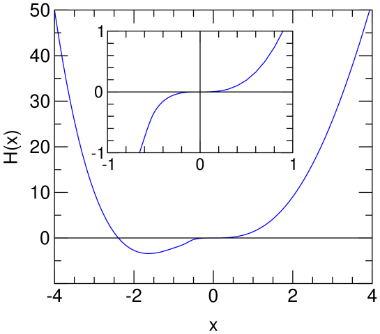
Figure 7: The universal function $H(x)$ for $-4\leq x\leq 4$. The solid line shows the result of the numerical calculation. The inset shows $H(x)$ for $-1\leq x\leq 1$ in more detail.

The inset shows $H(x)$ in the perturbative region $-1\leq x\leq 1$ in more detail. The local minimum for negative $x$ allows for a self-bound uniform system. (Repulsion at NLO was also observed in the modified loop expansion of Ref. WEHRBERGER90 .)

The energy per particle through NLO can be written in terms of $g$ and $x$ as

$$\frac{E}{N}=\frac{k_{\rm F}^{2}}{2M}\left[\left(\frac{3}{5}+\frac{2}{3}x\right)+\frac{1}{g}\left(\frac{3}{\pi}H(x)-\frac{2}{3}x+\frac{4}{35}(11-2\ln 2)x^{2}\right)\right]\ .$$ (56)

In Fig. 8, we show the energy per particle in units of the

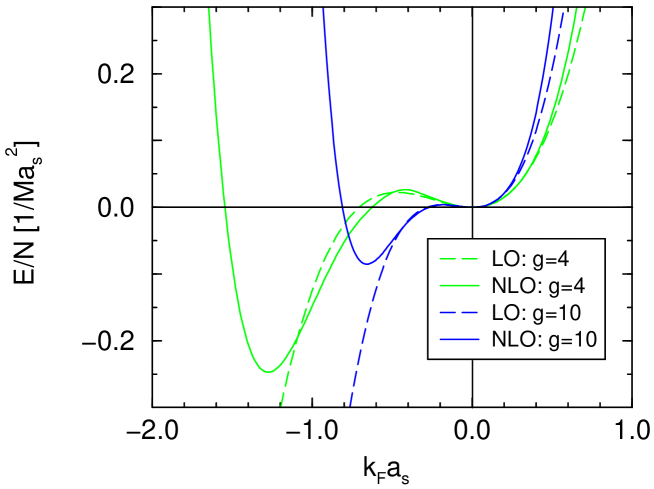
Figure 8: Energy per particle in units of $1/Ma_{s}^{2}$ at leading order (LO) and next-to-leading-order (NLO) in the $1/g$ expansion, for $g=4$ and $g=10$.

Fermi energy for two different values of $g$: $g=4$ and $g=10$. The dashed lines show the LO results while the solid lines show the NLO order results. The difference between LO and NLO gives an indication of where the expansion breaks down. The NLO result oscillates around the LO result in the vicinity of $k_{\rm F}a_{s}=0$ and grows without limit as $k_{\rm F}a_{s}\to\pm\infty$. As $g$ increases, the minimum becomes shallower and moves toward smaller values of $k_{\rm F}a_{s}$.

An important consideration is whether the energy calculated above actually corresponds to the true ground state of the system. There are two issues here: whether the state that evolves adiabatically from the noninteracting ground state is unstable to pairing near the Fermi surface and whether a homogeneous system is stable. There is no pairing instability if we restrict ourselves to repulsive interactions (e.g., a positive, natural-size scattering length), but pairing is inevitable with an attractive interaction (e.g., a negative scattering length or $x<0$). We will investigate the role of pairing in the EFT framework in future work. We note here that more conventional investigations typically find that the impact of pairing on the bulk properties (on which we focus) is small for natural scattering lengths Papenbrock:1998wb .

In order to investigate the stability of the homogeneous state, we calculate the compressibility JACKSON94

$$K = \frac{\partial}{\partial n}\left(n^{2}\frac{\partial}{\partial n}\frac{E}{N}\right)\,.$$ (57)

When the compressibility is positive, the system is stable with respect to infinitesimal long-range fluctuations in the density. When the compressibility is negative, however, long-range fluctuations will grow exponentially. As a consequence, the system will cluster and the homogeneous state is not the ground state. Using Eq. (36), the compressibility at leading order in the $1/g$ expansion is

$$K_{LO}=\frac{2k_{\rm F}^{2}}{3M}\left(\frac{gk_{\rm F}a_{s}}{\pi}+\frac{1}{2}\right)\,,$$ (58)

which turns negative for

$$x<x_{\rm crit}=-\frac{1}{2}\,.$$ (59)

As a consequence, the homogeneous system is unstable if $x<-1/2$. This constraint was previously obtained in Ref. JACKSON94 by identifying the radius of convergence for the exact fermion RPA energy, as well as from a variational argument. At next-to-leading order in the $1/g$ expansion, the compressibility $K_{NLO}$ follows from Eqs. (56) and (57) but we have not obtained an analytic expression. Furthermore, the point where the compressibility becomes negative now depends on $g$ and $k_{\rm F}a_{s}$ separately. Nevertheless, the numerical results for $K_{NLO}$ are close to the leading order values (59). For example, the next-to-leading order compressibility turns negative if $k_{\rm F}a_{s}<-0.73,-0.37,-0.15$ for $g=2,4,10$, respectively, as compared to $k_{\rm F}a_{s}<-0.79,-0.39,-0.16$ at leading order. This means that the self-bound uniform state given by the minimum of $E/N$ in Fig. 8 is not a stable ground state.

The above constraints can also be obtained directly from the effective action by looking for minima in Eq. (24) corresponding to a nonuniform state (with $\sigma_{c}=\sigma_{c}(x)$). The saddle points of the effective action determine where such minima appear. This analysis also determines the density fluctuation modes that destabilize the homogeneous state. In leading order, we require:

$$0=\frac{\delta^{2}}{\delta\sigma_{c}(x)\delta\sigma_{c}(y)}\Gamma_{LO}[\sigma_{c}(z)]=\frac{\delta^{2}}{\delta\sigma_{c}(x)\delta\sigma_{c}(y)}\left[\frac{g}{i}\,{\rm Tr}\ln[G_{H}^{-1}(x,y)]+\frac{C_{0}}{2}\int\!d^{4}x\,\sigma_{c}(x)^{2}\right]\,,$$ (60)

where $\sigma_{c}$ is a function of $x$. Using the identity

$$\frac{\delta^{2}}{\delta\sigma_{c}(x)\delta\sigma_{c}(y)}{\rm Tr}\ln[G_{H}^{-1}]=-C_{0}^{2}G_{H}(x,y)G_{H}(y,x)\,,$$ (61)

performing a Fourier transform with respect to $x-y$, and setting $q_{0}=0$, we obtain the equation

$$0=1-C_{0}\Pi_{0}(q_{0}=0,q)=1+x\left\{1-\frac{k_{\rm F}}{q}\left(1-\frac{q^{2}}{4k_{\rm F}^{2}}\right)\ln\left|\frac{1-q/(2k_{\rm F})}{1+q/(2k_{\rm F})}\right|\right\}\,,$$ (62)

whose solutions determine the long-range density fluctuation modes that destabilize the homogeneous system. The constraint obtained from solving Eq. (62) agrees with Eq. (59). At this order, the stability analysis in the effective action formalism is equivalent to identifying the poles in the $\sigma$ propagator $D_{\sigma}(q_{0}=0,q)$ from Eq. (48), as is done in conventional many-body approaches FETTER71 ; NEGELE88 . In principle, it is straightforward to extend the stability analysis to next-to-leading order by requiring

$$0=\frac{\delta^{2}}{\delta\sigma_{c}(x)\delta\sigma_{c}(y)}\left\{\Gamma_{LO}[\sigma_{c}(z)]+\Gamma_{NLO}[\sigma_{c}(z)]\right\}\,.$$ (63)

However, this analysis involves the evaluation of two-loop diagrams and is beyond the scope of this work.

V Bose limit

The EFT expansion is not limited, in general, to small values of $x$. For example, Eq. (56) implies that the $1/g$ expansion is valid for large $x$ if $g$ is also sufficiently large. The Bose limit, in which $x\rightarrow\infty$, provides an instructive example.

The energy density of a Bose system can be obtained from the energy density of a Fermi system by taking the limit $g\to\infty$, $k_{\rm F}\to 0$, but keeping $n=gk_{\rm F}^{3}/(6\pi^{2})$ constant JACKSON94 . Here $g$ is the degeneracy of an artificial “flavor” quantum number. This can be understood intuitively starting from a noninteracting Fermi system with large degeneracy. If the degeneracy $g$ is greater than the number of particles, the spatial state will be a symmetric wave function with all particles in the lowest momentum state. This is the same as the wave function of the Bose system with the same number of particles. If the interacting state evolves adiabatically from the noninteracting state, then the limiting Fermi system is the same as the interacting Bose system times a totally antisymmetric “flavor” wave function that has no physical consequences BRANDOW71 .

The Bose limit can be taken directly in Eq. (22), leading to the mean-field energy for a dilute Bose system. All terms vanish except for the part of the second term proportional to $g$, and the result is

$${\cal E}_{0}^{B}=\frac{2\pi a_{s}n^{2}}{M}\,,$$ (64)

in agreement with the literature FETTER71 . For higher-order terms, the analysis is more complicated since some contributions diverge as $g\to\infty$ and therefore need to be resummed. However, this is precisely the same resummation that is implemented in the one-loop effective action from the previous section.

In the Bose limit, the polarization insertion $\Pi_{0}$ [see Eq. (41)] has a simple analytic expression. In order to evaluate Eq. (42) most easily, we take the Bose limit of $\Pi_{0}$ before performing the $dy$ and $d^{4}q$ integrals. The polarization insertion can be written as

$$\Pi_{0}(q_{0},{\bf q})=g\int\frac{d^{3}p}{(2\pi)^{3}}\theta(k_{\rm F}-p)\left(\frac{\theta(|{\bf p}+{\bf q}|-k_{\rm F})}{q_{0}+\omega_{\bf p}-\omega_{{\bf p}+{\bf q}}+i\epsilon}-\frac{\theta(|{\bf p}-{\bf q}|-k_{\rm F})}{q_{0}-\omega_{\bf p}+\omega_{{\bf p}-{\bf q}}-i\epsilon}\right)\,.$$ (65)

If we let $|{\bf q}|=q\gg k_{\rm F}$ (or equivalently take $k_{\rm F}\to 0$), the $\theta$ functions involving ${\bf q}$ can be dropped. Expanding

$$\omega_{\bf p}-\omega_{{\bf p}\pm{\bf q}}=-\omega_{\bf q}(1+{\cal O}(p/q))\,,$$ (66)

the polarization insertion in the Bose limit becomes JACKSON94

$$\Pi_{0}^{B}(q_{0},{\bf q}) = g\int\frac{d^{3}p}{(2\pi)^{3}}\theta(k_{\rm F}-p)\left(\frac{1}{q_{0}-\omega_{\bf q}+i\epsilon}-\frac{1}{q_{0}+\omega_{\bf q}-i\epsilon}\right)$$ (67)

$$= \frac{2\omega_{\bf q}n}{(q_{0}-\omega_{\bf q}+i\epsilon)(q_{0}+\omega_{\bf q}-i\epsilon)}\,.$$

Thus $\Pi_{0}^{B}$ has simple poles in $q_{0}$ given by the noninteracting single-particle kinetic energy.

The ring sum leading to the integrand in Eq. (42) shifts the poles to the Bogoliubov quasiparticle energies:

$$\frac{y\Pi_{0}(q)}{1-y\Pi_{0}(q)}=\frac{y}{\Pi_{0}^{-1}(q)-y}=\frac{2\omega_{\bf q}ny}{q_{0}^{2}-\omega_{\bf q}^{2}-2\omega_{\bf q}ny+i\epsilon}=\frac{2\omega_{\bf q}ny}{q_{0}^{2}-\epsilon_{\bf q}^{2}+i\epsilon}\ ,$$ (68)

where

$$\epsilon_{\bf q}\equiv\sqrt{\omega_{\bf q}^{2}+2\omega_{\bf q}ny}\ .$$ (69)

The $dq_{0}$ integral in Eq. (42) is simply evaluated by contour integration and leads to

$${\cal E}_{1}^{B}=-\frac{\Gamma_{NLO}}{VT}=\frac{n}{2}\int_{0}^{C_{0}}\!dy\int\!\frac{d^{3}q}{(2\pi)^{3}}\frac{\omega_{\bf q}}{\epsilon_{\bf q}}=\frac{n}{2}\int_{0}^{C_{0}}\!dy\int\!\frac{d^{3}q}{(2\pi)^{3}}\frac{q^{2}}{q\sqrt{q^{2}+4Mny}}\ .$$ (70)

Note that an expansion of the final integrand in powers of $y$ would generate infrared (IR) divergences. The resummation of the one-loop fermion effective action is therefore required for bosons even in the low-density limit. This summation of ring diagrams because of IR divergences is analogous to the calculation of the correlation energy for a uniform electron gas, only in that case it is the interaction that is the source of the IR divergences FETTER71 .

The $d^{3}q$ integral in Eq. (70) can be evaluated in dimensional regularization with minimal subtraction. In particular, the formula

$$\int\!\frac{d^{d}k}{(2\pi)^{d}}\,\frac{k^{2}}{k\sqrt{k^{2}+\Lambda^{2}}}=\frac{\Gamma(-d/2)\Gamma(1/2+d/2)}{(4\pi)^{d/2}\Gamma(d/2)\Gamma(1/2)}(\Lambda^{2})^{d/2}$$ (71)

can be derived and applied for $d=3$ PESKIN95 . The end result is

$${\cal E}_{1}^{B} = \frac{n}{15\pi^{2}}(4Mn)^{3/2}C_{0}^{5/2}=\frac{2\pi a_{s}n^{2}}{M}\;\frac{128}{15\sqrt{\pi}}\sqrt{na_{s}^{3}}\,,$$ (72)

in agreement with the well-known result FETTER71 .

In principle, our numerical evaluation of the universal function $H(x)$, illustrated in Fig. 7, should match on to the Bose limit for large, positive $x\stackrel{{\scriptstyle>}}{{{}_{\sim}}}10$. We have not been able to demonstrate this matching. Indeed, the numerical continuation to large $x$ of $H(x)$ exhibits an entirely different behavior (e.g., it reaches a maximum and then turns negative, going to minus infinity with a different asymptotic power of $x$ then predicted by the Bose limit). It is not clear whether the problem is one of numerics (our calculations $x\stackrel{{\scriptstyle>}}{{{}_{\sim}}}10$ show severe round-off errors) or a more fundamental problem. Further investigations to resolve this issue are in progress.

VI Summary

In this paper, a system of fermions with short-range interactions at finite density is studied using the framework of effective field theory. The effective action formalism for fermions with auxiliary fields leads to a loop expansion in which particle-hole bubbles are resummed to all orders. For spin-independent interactions, the loop expansion is equivalent to a systematic expansion in $1/N$, where “$N$” is the spin-isospin degeneracy $g$. Thus we have a double expansion, in $1/g$ as well as $k_{\rm F}a_{s}$. The loop expansion differs from the dilute expansion described in Ref. HAMMER00 , even at leading order. At next-to-leading order, the expansion requires Hartree plus RPA contributions to the ground state FUKUDA94 ; WEHRBERGER90 ; TANAKA93 .

The formalism enables us to examine uniform systems for potential self-bound solutions. At next-to-leading order in $1/g$, the nonperturbative resummation leads for the uniform system to a non-trivial and non-analytic dependence on the Fermi momentum $k_{\rm F}$. There is a self-bound minimum within the radius of convergence of the EFT for sufficiently large $g$, but a stability analysis reveals that it is unstable to density fluctuations (e.g., clustering).

An interesting limit of the large $g$ expansion takes $g$ to infinity and $k_{\rm F}$ to zero, with the density $n$ held fixed. This limit reproduces the energy expansion for a dilute Bose gas, with the non-analytic dependence on $\sqrt{n}$ generated by the infinite summation of ring diagrams. We have not succeeded in reproducing the Bose limit starting from our explicit calculations for fermions, which may simply reflect the numerical difficulties in carrying out the limit but might also mean that there are subtleties we have not recognized. Work is in progress to resolve this issue.

While the present investigation illustrates some features of a systematic nonperturbative treatment of a Fermi system, we need to extend our treatment to include pairing and large scattering lengths to make contact with the physical systems of greatest interest. Investigations in these areas are in progress as well as work to adapt the effective action formalism to finite systems in the form of density functional theory PUGLIA02 .

Appendix A Higher-Order Two-Body and Many-Body Forces

In this appendix, we generalize the discussion of the $1/N$ expansion to consider higher-order two-body interactions ($C_{2}$, $C^{\prime}_{2}$, and so on) as well as many-body forces ($D_{0}$ and so on) that are present in a general EFT Lagrangian for the dilute system (see Ref. HAMMER00 for definitions and details):

$${\cal L} = \psi^{\dagger}\biggl{[}i\partial_{t}+\frac{\overrightarrow{\nabla}^{\,2}}{2M}\biggr{]}\psi-\frac{C_{0}}{2}(\psi^{\dagger}\psi)^{2}+\frac{C_{2}}{16}\Bigl{[}(\psi\psi)^{\dagger}(\psi\tensor{\nabla}^{2}\psi)+\mbox{ h.c.}\Bigr{]}$$ (73)

$$\hbox{}+\frac{C_{2}^{\prime}}{8}(\psi\tensor{\nabla}\psi)^{\dagger}\cdot(\psi\tensor{\nabla}\psi)-\frac{D_{0}}{6}(\psi^{\dagger}\psi)^{3}+\ldots\,.$$

There are various different ways of incorporating these interactions into the loop expansion, which correspond to different reorganizations of the original perturbative expansion, with different resummations of diagrams. The details of the system under consideration determine the power counting of the higher-order contributions; the most appropriate resummation will implement that power counting.

At the simplest level, we can incorporate all higher-order vertices perturbatively. This means that the only infinite summations based on large $g$ will be of the same subdiagrams with $C_{0}$ vertices we have already considered. We return to the generating functional in Eq. (2), but now with the full EFT Lagrangian for a dilute system with short-range interactions, and with Grassmann sources $\xi^{\dagger}$ and $\xi$ coupled to the fermion fields:

$$Z[\xi^{\dagger},\xi]=e^{-iE[\xi^{\dagger},\xi]}=\int{\cal D}{\psi^{\dagger}}{\cal D}\psi\,e^{i\int\!d^{4}x\,[{\cal L}+\xi^{\dagger}(x)\psi(x)+\psi^{\dagger}(x)\xi(x)]}\,,$$ (74)

where ${\cal L}$ is given by Eq. (16). [Spin indices are implicit in Eq. (74).] Functional derivatives with respect to the Grassmann sources can be used to generate the $n$-point fermion Green’s functions. If we isolate the quadratic part of the Lagrangian, this procedure generates the perturbative expansion of these functions in terms of the noninteracting fermion propagator (at finite chemical potential). The sum of closed, connected diagrams generated this way reproduces the perturbative expansion of the energy density from Ref. HAMMER00 .

In the present context, we use the Grassmann sources to remove all interaction terms from the path integral ${\cal L}_{I}(\psi^{\dagger},\psi)\rightarrow{\cal L}_{I}(-i\delta/\delta\xi,-i\delta/\delta\xi^{\dagger})$ except for the $C_{0}$ contact interaction. To carry out the procedure in Sect. II leading from Eq. (2) to Eq. (6), we need to incorporate the new Grassmann source terms. This is straightforward, since the identity

$$\psi^{\dagger}G^{-1}\psi+\psi^{\dagger}\xi+\xi^{\dagger}\psi=(\psi^{\dagger}+\xi^{\dagger}G)G^{-1}(\psi+G\xi)-\xi^{\dagger}G\xi\,,$$ (75)

and a shift in $\psi$ and $\psi^{\dagger}$ leaves the same integral as before (leading to the same ${\rm Tr}\ln$ term) plus a new term:

$$\exp\left[-i\int\!d^{4}x\,d^{4}y\,\xi^{\dagger}(x)G(x,y)\xi(y)\right]\,.$$ (76)

The new term still depends on $\sigma$ through $G(x,y)$.

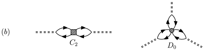
Figure 9: (a) New diagrams and (b) $\sigma$ propagator and vertex corrections generated by the perturbative inclusion of higher-order terms in the effective Lagrangian (73).

As in Eq. (11), we expand $\sigma$ about $\sigma_{c}$ in Eq. (76), which has the effect of expanding $G$ about $G_{H}$. The Grassmann sources $\xi$ and $\xi^{\dagger}$ in Eq. (76) have to match up with the derivatives in ${\cal L}_{I}(-i\delta/\delta\xi,-i\delta/\delta\xi^{\dagger})$ because the sources are set to zero in the end. This dictates how the higher-order vertices (e.g., $C_{2}$ and $D_{0}$) appear in Feynman diagrams attached to $G_{H}$ propagators. The quadratic term in $\eta$ can be directly incorporated into Eq. (26) while the higher-order terms generate additional connected 1PI-diagrams. (For consistency, one should expand the $\sigma$ propagators perturbatively in the higher-order interactions.) The $\eta$-independent part of Eq. (76), which has $G\rightarrow G_{H}$, generates tadpole-like diagrams with the new vertices, such as those illustrated in Fig. 9(a), as well as higher-order contributions. The new diagrams based on the $\eta$ expansion can be constructed by breaking every possible $G_{H}$ line (including those buried in the $\sigma$ propagator) and connecting the broken ends to the new vertices. Examples of $\sigma$-propagator and $V_{3}$ vertex corrections are shown in Fig. 9(b).

An alternative approach to incorporating higher-order two-body and many-body interactions is to generalize the $\sigma$ Lagrangian in Eq. (29) to include $\sigma^{3}$ and higher-order self-interactions, as well as terms with gradients (but not time derivatives) acting on $\sigma$. If we put back the fermion path integral and eliminate the $\sigma$ field by iteratively applying its Euler-Lagrange equation via field redefinitions, we reproduce an infinite subset of the terms in the general dilute effective Lagrangian. For example, we recover the $D_{0}$ vertex and the combination of $C_{2}$ and $C^{\prime}_{2}$ corresponding to a term proportional to $\nabla(\psi^{\dagger}\psi)\cdot\nabla(\psi^{\dagger}\psi)$. In general, we find all interaction terms with $\psi^{\dagger}_{\alpha}\psi_{\alpha}$ to some power and gradients acting on such factors (these are terms that depend only on the momentum transfer between the fermions).

The generalized $\sigma$ Lagrangian can be expanded about $\sigma_{c}$ as before, with the new terms treated to all orders (analogous to the treatment of the linear sigma model in Ref. PESKIN95 ) or as perturbative corrections. In the former case, the strict power counting in which all diagrams contribute at a given order in $1/g$ is violated unless the counting of the coefficient of the $\sigma^{3}$ term, $\widetilde{D}_{0}\propto D_{0}$, is promoted to ${\cal O}(1/g^{2})$ from ${\cal O}(1/g^{4})$ in the perturbative case. The latter case is similar to the discussion above, except that a given higher-order term in the generalized $\sigma$ Lagrangian will be equivalent to a selective summation of higher-order terms expressed in the basis of fermion fields alone.

References

- (1) S. Weinberg, Physica 96A, 327 (1979).
- (2) G.P. Lepage, “What is Renormalization?”, in From Actions to Answers (TASI-89), edited by T. DeGrand and D. Toussaint (World Scientific, 1989); arXiv:nucl-th/9706029.
- (3) D.B. Kaplan, arXiv:nucl-th/9506035.
- (4) Proceedings of the Joint Caltech/INT Workshop: Nuclear Physics with Effective Field Theory, ed. R. Seki, U. van Kolck, and M.J. Savage (World Scientific, 1998).
- (5) Proceedings of the INT Workshop: Nuclear Physics with Effective Field Theory II, ed. P.F. Bedaque, M.J. Savage, R. Seki, and U. van Kolck (World Scientific, 2000).
- (6) U. van Kolck, Prog. Part. Nucl. Phys. 43, 337 (1999).
- (7) S.R. Beane, P.F. Bedaque, W.C. Haxton, D.R. Phillips, and M.J. Savage, “From Hadrons to Nuclei: Crossing the Border”, in At the Frontier of Particle Physics, vol. 1, ed. M. Shifman (World Scientific, 2001). arXiv:nucl-th/0008064.
- (8) P.F. Bedaque and U. van Kolck, arXiv:nucl-th/0203055.
- (9) H.-W. Hammer and R.J. Furnstahl, Nucl. Phys. A 678, 277 (2000) [arXiv:nucl-th/0004043].
- (10) A.L. Fetter and J.D. Walecka, Quantum Theory of Many-Particle Systems (McGraw–Hill, 1971).
- (11) R.F. Bishop, Ann. Phys. (NY) 77, 106 (1973).
- (12) E. Braaten and A. Nieto, Phys. Rev. B 55, 8090 (1997); Eur. Phys. J. B 11, 143 (1999).
- (13) R.J. Furnstahl and H.-W. Hammer, Phys. Lett. B 531, 203 (2002) [arXiv:nucl-th/0108069].
- (14) R.J. Furnstahl, H.-W. Hammer, and N. Tirfessa, Nucl. Phys. A 689, 846 (2001) [arXiv:nucl-th/0010078].
- (15) U. van Kolck, Nucl. Phys. A 645, 273 (1999) [arXiv:nucl-th/9808007].
- (16) D.B. Kaplan, M.J. Savage, and M.B. Wise, Nucl. Phys. B 534, 329 (1998) [arXiv:nucl-th/9802075].
- (17) P.F. Bedaque, H.-W. Hammer, and U. van Kolck, Phys. Rev. Lett. 82, 463 (1999) [arXiv:nucl-th/9809025]; Nucl. Phys. A 646, 444 (1999) [arXiv:nucl-th/9811046].
- (18) P.F. Bedaque, H.-W. Hammer, and U. van Kolck, Nucl. Phys. A 676, 357 (2000) [arXiv:nucl-th/9906032].
- (19) J.V. Steele, arXiv:nucl-th/0010066.
- (20) S. Coleman, Aspects of Symmetry (Cambridge Univ. Press, New York, 1988).
- (21) E. Brezin and S.R. Wadia, The Large N Expansion In Quantum Field Theory And Statistical Physics: From Spin Systems To Two-Dimensional Gravity, (World Scientific, 1993)
- (22) F. Calogero and A. Degasperis, Phys. Rev. A 11, 265 (1975).
- (23) B. Yoon and J.W. Negele, Phys. Rev. A 16, 1451 (1977).
- (24) K. Tanaka, W. Bentz, and A. Arima, Nucl. Phys. A 555, 151 (1993).
- (25) J.W. Negele and H. Orland, Quantum Many-Particle Systems (Addison–Wesley, 1988).
- (26) R.J. Furnstahl and B.D. Serot, Nucl. Phys. A 673, 298 (2000) [arXiv:nucl-th/9912048].
- (27) J.V. Steele and R.J. Furnstahl, Nucl. Phys. A 645, 439 (1999) [arXiv:nucl-th/9808022].
- (28) R.J. Furnstahl, Nucl. Phys. A 706, 85 (2002) [arXiv:nucl-th/0112085] and references therein.
- (29) R.J. Furnstahl and B.D. Serot, Comments Nucl. Part. Phys. 2, A23 (2000) [arXiv:nucl-th/0005072].
- (30) G. Gentile, Nuovo Cimento 17, 492 (1940); 19, 109 (1942).
- (31) G. Schubert, Z. Naturforsch. 1, 113 (1946).
- (32) B.H. Brandow, Ann. Phys. (NY) 64, 21 (1971).
- (33) A.D. Jackson and T. Wettig, Phys. Rep. 237, 325 (1994).
- (34) M.E. Peskin and D.V. Schroeder, An Introduction to Quantum Field Theory (Addison–Wesley, 1995).
- (35) R. Fukuda, T. Kotani, Y. Suzuki, and S. Yokojima, Prog. Theor. Phys. 92, 833 (1994).
- (36) C. Itzykson and J.-B. Zuber, Quantum Field Theory (McGraw–Hill, 1980).
- (37) S. Weinberg, The Quantum Theory of Fields: vol. II, Modern Applications (Cambridge University Press, 1996).
- (38) J. Hubbard, Phys. Rev. Lett. 3, 77 (1959); R.L. Stratonovich, Dokl. Akad. Nauk S.S.R.S. 115, 1907 (1957).
- (39) N. Weiss, Phys. Rev. D 27, 899 (1983).
- (40) K. Wehrberger, R. Wittman, and B.D. Serot, Phys. Rev. C 42, 2680 (1990).
- (41) T. Papenbrock and G.F. Bertsch, Phys. Rev. C 59, 2052 (1999).
- (42) S. Puglia and R.J. Furnstahl, in preparation.