Quasiparticle Properties in Effective Field Theory

Abstract

The quasiparticle concept is an important tool for the description of many-body systems. We study the quasiparticle properties for dilute Fermi systems with short-ranged, repulsive interactions using effective field theory. We calculate the proper self-energy contributions at order $(k_{F}/\Lambda)^{3}$, where $\Lambda$ is the short-distance scale that sets the size of the effective range parameters and $k_{F}$ the Fermi momentum. The quasiparticle energy, width, and effective mass to ${\cal O}((k_{F}/\Lambda)^{3})$ are derived from the calculated self-energy.

I Introduction

A relatively new approach to many-body phenomena is that of effective field theory (EFT). The EFT approach is designed to exploit the separation of scales in physical systems WEINBERG79 ; LEPAGE89 ; KAPLAN95 . Only low-energy (or long-range) degrees of freedom are included explicitly, with the rest parametrized in terms of the most general local (contact) interactions. Using renormalization, the influence of high-energy states on low-energy observables is captured in a small number of low-energy constants. Thus, the EFT describes universal low-energy physics independent of detailed assumptions about the short-distance dynamics. Furthermore, the application of EFT methods to many-body problems gives a consistent organization of many-body corrections, with reliable error estimates, and insight into the analytic structure of observables. EFT provides a model independent description of finite density observables in terms of parameters that can be fixed from scattering in the vacuum. In low-energy particle and nuclear physics, EFT methods have successfully been applied to mesonic systems GaL85 , processes with one baryon Mei00 , and more recently also to processes involving two and more baryons BEANE99 ; Bedaque:2002mn .

A description in terms of quasiparticles is central to many approaches to the many-body problem. It has proven useful in many physical systems from condensed matter physics to nuclear physics NEGELE88 ; FETTER71 . If the states of the noninteracting system are gradually transformed into the interacting states when the interactions are switched on adiabatically, the excitations of the interacting system near the Fermi surface (the quasiparticles) have the same character as the excitations of the noninteracting Fermi gas. This is the basic assumption underlying Landau’s theory of Fermi liquids Landau56 ; Noz97 . The assumption holds, e.g., for a dilute Fermi system with repulsive, short-ranged interactions. This system has been a benchmark problem for many-body techniques for a long time efimov ; baker ; bishop ; HAMMER00 . In particular, the low density allows for a controlled expansion in $k_{F}a_{s}$ where $k_{F}$ is the Fermi momentum and $a_{s}$ is the S-wave scattering length of the fermions. In the framework of EFT, this corresponds to an expansion in $k_{F}/\Lambda$ where $\Lambda$ is the breakdown scale of the EFT. For a natural system the scale $\Lambda$ sets the scale of $a_{s}$ and all other effective range parameters. Initially, there were not many applications for this model system, but recently ultra-cold Fermi gases of atoms have been achieved jin99 ; hulet01 . The dilute Fermi gas also serves as a simpler test case on the way to an EFT description of nuclear matter. The quasiparticle properties in the dilute Fermi gas to ${\cal O}((k_{F}/\Lambda)^{2})$ were first calculated by Galitskii GALITSKII . An incomplete numerical study of the quasiparticle properties to ${\cal O}((k_{F}/\Lambda)^{3})$ was carried out in Ref. bund . In Ref. SARTOR80 , the proper self-energy was calculated off-shell to ${\cal O}((k_{F}/\Lambda)^{2})$ and the momentum dependence of the effective mass was studied in detail.

In this paper, we perform the first complete calculation of the quasiparticle properties in the dilute Fermi gas to ${\cal O}((k_{F}/\Lambda)^{3})$ in the low-density expansion. At this order both the S-wave effective range $r_{s}$ and the P-wave scattering length $a_{p}$ contribute. We calculate the quasiparticle energies $\epsilon_{k}$, width $\gamma_{k}$, and effective mass $M^{*}$. As a check, we also calculate the chemical potential $\mu$ and the energy per particle and compare with the known results efimov ; baker ; bishop ; HAMMER00 . The outline of this paper is as follows. In Sec. II we repeat briefly the elements of an EFT approach to dilute Fermi systems. In Sec. III, we calculate the proper self-energy at order $(k_{F}/\Lambda)^{3}$. The quasiparticle properties to ${\cal O}((k_{F}/\Lambda)^{3})$ are derived from the self-energy in Sec. IV. In Sec. V, we summarize and present our conclusions.

II Effective Field Theory for Dilute Fermi Systems

In this section, we review briefly the EFT approach for dilute Fermi systems. We will restrict ourselves to repulsive interactions. An EFT for such a system is discussed in detail in Ref. HAMMER00 . In contrast to more traditional many-body approaches efimov ; baker ; bishop the EFT for the dilute Fermi gas is fully perturbative. It is appropriate to consider a natural EFT for heavy, nonrelativistic fermions of mass M with spin-independent interactions whose strength is correctly determined by naive dimensional analysis. The scale of all effective range parameters is set by $1/\Lambda$, where $\Lambda$ is the breakdown scale of the theory. For momenta $k\ll\Lambda$, all interactions appear short-ranged and can be modeled by contact terms. Therefore, we consider a local Lagrangian for a nonrelativistic fermion field that is invariant under Galilean, parity, and time-reversal transformations:

$${\cal L} = \psi^{\dagger}\biggl{[}i\partial_{t}+\frac{\overrightarrow{\nabla}^{2}\!}{2M}\biggr{]}\psi-\frac{C_{0}}{2}(\psi^{\dagger}\psi)^{2}+\frac{C_{2}}{16}\Bigl{[}(\psi\psi)^{\dagger}(\psi\tensor{\nabla}^{2}\psi)+\mbox{ H.c.}\Bigr{]}$$ (1)

$$+\frac{C_{2}^{\prime}}{8}(\psi\tensor{\nabla}\psi)^{\dagger}\cdot(\psi\tensor{\nabla}\psi)+\ldots\,,$$

where $\tensor{\nabla}=\overleftarrow{\nabla}-\overrightarrow{\nabla}$ is the Galilean invariant derivative and H.c. denotes the Hermitian conjugate. Higher-order time derivatives are not included, since it is most convenient for our purposes to eliminate them in favor of spatial gradients.

For convenience, we choose dimensional regularization with minimal subtraction as our renormalization scheme. Calculating the two-particle scattering amplitude in the vacuum to ${\cal O}((k/\Lambda)^{3})$, the coefficients $C_{2i}$ can be determined by matching to the leading coefficients of the effective range expansion (see, e.g., Ref. HAMMER00 for details). Thus, the $C_{2i}$ can be expressed completely in terms of the effective range parameters:

$$C_{0}=\frac{4\pi a_{s}}{M},\qquad C_{2}=C_{0}\frac{a_{s}r_{s}}{2},\qquad\mbox{and}\qquad C_{2}^{\prime}=\frac{4\pi a_{p}^{3}}{M},$$ (2)

where $a_{s}$, $a_{p}$ and $r_{s}$ are the S- and P-wave scattering lengths and S-wave effective range, respectively.

We now turn to the finite density system. First, consider a noninteracting Fermi gas. The single particle states of the system are characterized by a momentum $k$ and a spin quantum number $s$. In particular, the ground-state of the system is the state in which all single-particle states with momentum less than the Fermi momentum $k_{F}$ are occupied and all other single-particle states are empty. Any excited state of the system can be created by removing particles with momentum less than $k_{F}$ and adding particles with momentum greater than $k_{F}$.

Now we turn on the interactions. We assume that there is a one-to-one correspondence between the states of the noninteracting Fermi gas and those of the interacting system if the interaction is switched on adiabatically. Note that this is not the case if the interaction is attractive. In this case, it is energetically favorable to form Cooper pairs and our calculation does not lead to the correct ground state. The elementary excitations of the interacting system correspond thus to the particle and hole excitations of the noninteracting Fermi gas, and are referred to as quasiparticles and quasiholes, respectively. Information about the properties of quasiparticles is contained in the proper self-energy $\Sigma^{*}(k_{0},{\bf k})$. In terms of diagrams, the proper self-energy represents one-particle irreducible and amputated self-energy insertions. The proper self-energy is related to the full Green’s function $G_{\alpha\beta}(\tilde{k})$ by Dyson’s equation FETTER71 :

$$G_{\alpha\beta}(\tilde{k})=G^{0}_{\alpha\beta}(\tilde{k})+G^{0}_{\alpha\lambda}(\tilde{k})\Sigma^{*}(\tilde{k})_{\lambda\mu}G_{\mu\beta}(\tilde{k})\,,$$ (3)

where ${\tilde{k}}\equiv(k_{0},{\bf k})$, $\alpha,\beta,...$ are spin indices, and the subscript $0$ denotes the noninteracting Green’s function defined in Eq. (5) below. For spin-independent interactions this equation can be solved analytically to give:

$$G_{\alpha\beta}(\tilde{k})=\frac{\delta_{\alpha\beta}}{k_{0}-{\bf k}^{2}/(2M)-\Sigma^{*}(\tilde{k})}\,.$$ (4)

Here, we only repeat the Feynman rules for the proper self-energy: The vertices that follow from the Lagrangian (1) are illustrated in Fig. 1. For short-range interactions the direct and exchange contributions differ only by a spin degeneracy factor. As a consequence, it is convenient to use so-called “Hugenholtz” diagrams where the direct and exchange contributions are combined in local four-fermion vertices.

Figure 1: Feynman rules for the vertices arising from the Lagrangian (1). The relative momenta of the incoming and outgoing particles, are $2{\bf k}$ and $2{\bf k}^{\prime}$, respectively. The spin indices have been suppressed.

The Feynman rules are HAMMER00 :

1. Write down all Hugenholtz diagrams that scale with a given order in $k_{F}$ as determined by the power counting rules given below.

2. Assign nonrelativistic four-momenta (frequency and three-momentum) to all lines and enforce four-momentum conservation at each vertex.

3. For each vertex, include the corresponding expression from Fig. 1. For spin-independent interactions, the two-body vertices have the structure $(\delta_{\lambda\gamma}\delta_{\beta\delta}+\delta_{\lambda\delta}\delta_{\beta\gamma})$, where $\lambda,\beta$ are the spin indices of the incoming lines and $\gamma,\delta$ are the spin indices of the outgoing lines. For each internal line include a factor $iG_{0}(\widetilde{k})_{\lambda\gamma}$, where $\widetilde{k}\equiv(k_{0},{\bf k})$ is the four-momentum assigned to the line, $\lambda$ and $\gamma$ are spin indices, and

   $$iG_{0}(\widetilde{k})_{\lambda\gamma}=i\delta_{\lambda\gamma}\left(\frac{\theta(k-k_{F})}{k_{0}-{\bf k}^{2}/(2M)+i\epsilon}+\frac{\theta(k_{F}-k)}{k_{0}-{\bf k}^{2}/(2M)-i\epsilon}\right)\ .$$ (5)

4. Perform the spin summations in the diagram. In every closed fermion loop, substitute a spin degeneracy factor $-g$ for each $\delta_{\lambda\lambda}$.

5. Integrate over all independent momenta with a factor $\int\!d^{4}k/(2\pi)^{4}$ where $d^{4}k\equiv dk_{0}\,d^{3}k$. If the spatial integrals are divergent, they are defined in $D$ spatial dimensions and renormalized using minimal subtraction as discussed in Ref. HAMMER00 . For a tadpole line with four-momentum $\tilde{k}$, multiply by $\exp(ik_{0}\eta)$ and take the limit $\eta\to 0^{+}$ after the contour integrals have been carried out. This procedure automatically takes into account that such lines must be hole lines.

6. Multiply every Hugenholtz diagram by the appropriate symmetry factor.

Furthermore, we repeat the power-counting rules that determine the power of $k_{F}$ with which a given diagram scales:

• for every propagator a factor $M/k_{F}^{2}$ ,

• for every loop integration a factor of $k_{F}^{5}/M$ ,

• for every n-body vertex with $2i$ derivatives a factor $k_{F}^{2i}/(M\Lambda^{2i+3n-5})$ ,

where $\Lambda$ is the breakdown scale of the theory which is determined by the physics not included in the EFT (such as the mass of a heavy exchanged particle). Thus, $k_{F}$ has to be much smaller than $\Lambda$, which is just the case for low density systems with short-range interactions where $\rho\propto k_{F}^{3}\ll 1/a_{s}^{3}\sim\Lambda^{3}$. In the above power counting rules, the external momentum ${\bf k}$ in $\Sigma^{*}$ is also counted as order $k_{F}$. This is appropriate, since the external momentum is converted to $k_{F}$ if observables like the energy density or quasiparticle properties are calculated. All proper self-energy diagrams have an overall factor of the Fermi energy $k_{F}^{2}/(2M)$ which we suppress in the labeling of different orders. The leading order contribution then starts at ${\cal O}(k_{F}/\Lambda)$. As a consequence, the expansion of $\Sigma^{*}$ reads:

$$\Sigma^{*}(k_{0},{\bf k})=\Sigma^{*}_{1}+\Sigma^{*}_{2}(k_{0},{\bf k})+\Sigma^{*}_{3}(k_{0},{\bf k})+\ldots\,,$$ (6)

where the lower index indicates the corresponding power of $k_{F}/\Lambda$. In a homogeneous system $\Sigma^{*}(k_{0},{\bf k})$ depends only on $k=|{\bf k}|$. The expressions for the self-energy through ${\cal O}((k_{F}/\Lambda)^{2})$ for $k_{0}=k^{2}/(2M)$ (sometimes called “on shell”) were first calculated by Galitskii GALITSKII . The general expressions for arbitrary $k_{0}$ were obtained in Ref. SARTOR80 . For completeness, we quote the on-shell expressions for $\Sigma^{*}_{1}$ and $\Sigma^{*}_{2}$ which will be needed later on:

$$\Sigma^{*}_{1}=\frac{k_{F}^{2}}{2M}(g-1)\frac{4}{3\pi}(k_{F}a_{s})\,,$$ (8)

$${\rm Re}\,\Sigma^{*}_{2}(\mbox{$\frac{k^{2}}{2M}$},k)=\frac{k_{F}^{2}}{2M}(g-1)(k_{F}a_{s})^{2}\frac{4}{15\pi^{2}}\frac{1}{v}\biggl{[}11v+2v^{5}\ln\biggl{|}\frac{v^{2}}{v-1}\biggr{|}$$

$$\quad\qquad-10(v^{2}-1)\ln\biggl{|}\frac{v+1}{v-1}\biggr{|}-(2-v^{2})^{5/2}\ln\biggl{|}\frac{1+v\sqrt{2-v^{2}}}{1-v\sqrt{2-v^{2}}}\biggr{|}\biggr{]}\,,$$

$$0<k<k_{F}:\, {\rm Im}\,\Sigma^{*}_{2}(\mbox{$\frac{k^{2}}{2M}$},k)=(g-1)\frac{k_{F}^{2}}{4\pi M}(k_{F}a_{s})^{2}(1-v^{2})^{2}\,,$$ (9)

$$k_{F}<k<\sqrt{2}k_{F}:\, {\rm Im}\Sigma^{*}_{2}(\mbox{$\frac{k^{2}}{2M}$},k)=(1-g)\frac{k_{F}^{2}}{15\pi M}(k_{F}a_{s})^{2}\frac{1}{v}\biggl{(}5v^{2}-7+2(2-v^{2})^{5/2}\biggr{)}\,,$$ (10)

with $v=k/k_{F}$. If the imaginary parts in Eqs. (9) and (10) are expanded around the Fermi surface at $v=1$, the first nonvanishing contribution occurs at ${\cal O}((1-v)^{2})$ as required by Luttinger’s general theorem LUTTINGER61 . In the next section, we calculate the proper self-energy contribution $\Sigma^{*}_{3}$ at ${\cal O}((k_{F}/\Lambda)^{3})$ for $k_{0}=k^{2}/(2M)$. As we will show in Section IV, only the on-shell value of $\Sigma^{*}_{3}$ is required for the quasiparticle properties.

III Proper Self-Energy at ${\cal O}((k_{F}/\Lambda)^{3})$

In this section, we calculate the contribution to the proper self-energy at ${\cal O}((k_{F}/\Lambda)^{3})$: $\Sigma^{*}_{3}$.

Figure 2: Hugenholtz diagrams contributing to $\Sigma^{*}_{3}(k_{0},k)$. Solid lines indicate noninteracting fermion propagator (5), while dotted lines indicate amputated fermion propagators. The expressions for the vertices are given in Fig. 1.

$\Sigma^{*}_{(3)}(k_{0},k)$ is given by the nine diagrams in shown Fig. 2. We will omit the calculational details in this section and show a sample calculation of diagram (7) in Appendix A. Diagrams (1) to (3) vanish when evaluated. Diagrams (4) and (5) can be related to the derivative of $\Sigma^{*}_{2}(k_{0},k)$ with respect to $k_{0}$:

$$\Sigma^{*}_{3(4)}(k_{0},k)+\Sigma^{*}_{3(5)}(k_{0},k)=-\Sigma^{*}_{1}\left.\frac{\partial\Sigma^{*}_{2}(k_{0},k)}{\partial k_{0}}\right|_{k_{0}=\frac{k^{2}}{2M}}\,.$$ (11)

They do not contribute the quasiparticle properties at ${\cal O}((k_{F}/\Lambda)^{3})$ as will be shown in the next section. Diagrams (8) and (9) can be evaluated analytically and give purely real results. For diagrams (6) and (7), we could not obtain analytical results; instead we have simplified the analytical expressions as far as possible and calculated them numerically using the Vegas Monte Carlo integration routine vegas . Below, we give parametrizations for the contributions of diagrams (6) and (7) to $\Sigma^{*}_{3}$ from a fit to the numerical results. We have fitted the results for different external momenta $k$ to polynomials in $(k_{F}-k)$ in an expansion around the Fermi surface. We have truncated the expansion at the order in $(k_{F}-k)$ at which adding another term does not improve the $\chi^{2}$ of the fit anymore. According to this criterion a polynomial of seventh degree is sufficient for the real parts, while the imaginary parts require a polynomial of ninth degree in $(k_{F}-k)$. The results for the contributions to the proper self-energy at ${\cal O}((k_{F}/\Lambda)^{3})$ are:

$$\hbox{Re}\,\Sigma^{*}_{3(6)}(\mbox{$\frac{k^{2}}{2M}$},k) = \frac{k_{F}^{2}}{2M}(g-1)(g-3)\frac{2^{3}}{\pi^{3}}(k_{F}a_{s})^{3}~{}\biggl{\{}0.5908-0.8829(1-v)$$ (12)

$$\qquad+0.2140(1-v)^{2}+3.7284(1-v)^{3}-2.7392(1-v)^{4}$$

$$\qquad-4.7509(1-v)^{5}+7.0977(1-v)^{6}-2.6709(1-v)^{7}\biggr{\}}\,,$$

$$\hbox{Re}\,\Sigma^{*}_{3(7)}(\mbox{$\frac{k^{2}}{2M}$},k) = \frac{k_{F}^{2}}{2M}(g-1)\frac{2^{3}}{\pi^{3}}(k_{F}a_{s})^{3}\biggl{\{}0.7811+1.0589(1-v)$$ (13)

$$\qquad+0.4160(1-v)^{2}+1.9942(1-v)^{3}-3.1936(1-v)^{4}$$

$$\qquad-4.8352(1-v)^{5}+9.6964(1-v)^{6}-4.1846(1-v)^{7}\biggr{\}}~{},$$

$$\hbox{Re}\,\Sigma^{*}_{3(8)}(\mbox{$\frac{k^{2}}{2M}$},k) = \frac{k_{F}^{2}}{2M}\frac{(g+1)}{\pi}(k_{F}a_{p})^{3}\biggl{\{}\frac{1}{5}+\frac{1}{3}v^{2}\biggr{\}}\,,$$ (14)

$$\hbox{Re}\,\Sigma^{*}_{3(9)}(\mbox{$\frac{k^{2}}{2M}$},k) = \frac{k_{F}^{2}}{2M}\frac{(g-1)}{2\pi}\,k_{F}^{3}a_{s}^{2}r_{s}\,\biggl{\{}\frac{1}{5}+\frac{1}{3}v^{2}\biggr{\}}\,,$$ (15)

$$\hbox{Im}\,\Sigma^{*}_{3(6)}(\mbox{$\frac{k^{2}}{2M}$},k) = \frac{k_{F}^{2}}{2M}\frac{16(g-1)(g-3)}{\pi^{2}}(k_{F}a_{s})^{3}\biggl{[}\biggl{\{}-0.0065(1-v)^{2}-1.0778(1-v)^{3}$$ (16)

$$\;+5.2913(1-v)^{4}-13.0528(1-v)^{5}+18.7234(1-v)^{6}$$

$$\;-15.4468(1-v)^{7}+6.7036(1-v)^{8}-1.1653(1-v)^{9}\biggr{\}}\theta(1-v)$$

$$\;+\biggl{\{}-0.0700(1-v)^{2}-5.3866(1-v)^{3}-84.0177(1-v)^{4}$$

$$\;-721.4519(1-v)^{5}-3546.7045(1-v)^{6}-9902.6272(1-v)^{7}$$

$$\;-14617.8867(1-v)^{8}-8855.7811(1-v)^{9}\biggr{\}}\theta(v-1)\biggr{]}\,,$$

$$\hbox{Im}\,\Sigma^{*}_{3(7)}(\mbox{$\frac{k^{2}}{2M}$},k) = \frac{k_{F}^{2}}{2M}\frac{8(g-1)}{\pi^{2}}(k_{F}a_{s})^{3}\biggl{[}\biggl{\{}-0.3835(1-v)^{2}+3.1281(1-v)^{3}$$ (17)

$$\;-7.1868(1-v)^{4}+12.1392(1-v)^{5}-16.3114(1-v)^{6}$$

$$\;+14.4972(1-v)^{7}-7.2813(1-v)^{8}+1.5639(1-v)^{9}\biggr{\}}\theta(1-v)$$

$$\;+\biggl{\{}0.3715(1-v)^{2}+8.0530(1-v)^{3}+77.9691(1-v)^{4}$$

$$\;+532.4357(1-v)^{5}+2237.8794(1-v)^{6}+5462.8759(1-v)^{7}$$

$$\;+7100.2592(1-v)^{8}+3791.8271(1-v)^{9}\biggr{\}}\theta(v-1)\biggr{]}~{},$$

$$\hbox{Im}\,\Sigma^{*}_{3(8)}(\mbox{$\frac{k^{2}}{2M}$},k) = 0\,,$$

$$\hbox{Im}\,\Sigma^{*}_{3(9)}(\mbox{$\frac{k^{2}}{2M}$},k) = 0\,,$$ (18)

where $v=k/k_{F}$. In Eqs. (12), (13), (16), and (17), we give the numerical constants to four decimal places to ensure that the parametrizations differ from the exact numerical values by less than $1\%$. Also, note that the parametrizations for the imaginary parts start with the $(1-v)^{2}$ term and satisfy Luttinger’s theorem LUTTINGER61 by construction.

IV Quasiparticle Properties

The elementary excitations of the interacting system correspond to the particle and hole excitations of the noninteracting Fermi gas, and are referred to as quasiparticles and quasiholes, respectively. Information about the properties of quasiparticles is contained in the proper self-energy $\Sigma^{*}(k_{0},k)$. The singularities of the full Green’s function (4) determine the excitation energies $\epsilon_{k}$ of the system and their corresponding widths $\gamma_{k}$. In the quasiparticle approximation, the full Green’s function (4) can be written as

$$G(k_{0},k)=\frac{Z}{k_{0}-\epsilon_{k}-i\gamma_{k}}\quad+\quad\mbox{regular terms}\,,$$ (19)

where $Z$ is the wave function renormalization. To determine $\epsilon_{k}$ and $\gamma_{k}$, we have to solve the equation:

$$\epsilon_{k}+i\gamma_{k}-\frac{k^{2}}{2M}-\Sigma^{*}(\epsilon_{k}+i\gamma_{k},k)=0\,,$$ (20)

while the wave function renormalization $Z$ is given by

$$Z^{-1}=1-\left.\frac{\partial\Sigma^{*}(k_{0},k)}{\partial k_{0}}\right|_{k_{0}=\epsilon_{k}+i\gamma_{k},\,k=k_{F}}\,.$$ (21)

The effective mass $M^{*}$ of the quasiparticle is defined using the group velocity of a quasiparticle state at the Fermi surface; that is the slope of the excitation energy at $p=k_{F}$ FETTER71 :

$$M^{*}=k_{F}\biggl{(}\frac{\partial\epsilon_{k}}{\partial k}\biggl{|}_{k=k_{F}}\biggr{)}^{-1}~{}.$$ (22)

The effective mass can be extracted from the heat capacity of the system in the zero temperature limit FETTER71 :

$$\frac{C_{V}}{V}=\frac{k_{B}^{2}TM^{*}k_{F}}{3}\quad\hbox{as}\quad T\rightarrow 0~{}.$$ (23)

Various other observables can be computed from these results as well. The chemical potential $\mu$ describes the minimal energy required to add an additional particle to a system. Consequently, it is given by the quasiparticle excitation energy at the Fermi surface:

$$\mu=\left.\epsilon_{k}\right|_{k=k_{F}}\,.$$ (24)

Another observable, which allows a simple check of the calculated excitation energies, is the energy per particle. One can compute the energy per particle directly from the proper self-energy $\Sigma^{*}(p_{0},p)$. It is easier, however, to use thermodynamical identities. The chemical potential at zero entropy $S$ is related to the exact ground-state energy $E$ by the thermodynamic identity:

$$\mu=\biggl{(}\frac{\partial E}{\partial N}\biggr{)}_{V}\quad\hbox{at}\quad S=0~{}.$$ (25)

Integrating this equation at a constant volume $V$ and zero entropy gives:

$$E=\int_{0}^{N}\hbox{d}N^{\prime}\mu(S=0,V,N^{\prime})~{}.$$ (26)

Since the $N$ dependence of $\mu$ is hidden in the Fermi momentum $k_{F}$ through the relation $k_{F}=(6\pi^{2}N/gV)^{1/3}$, the energy per particle is easily evaluated by multiplying each term in the chemical potential of order $(k_{F})^{\lambda}$ by a factor of $3/(3+\lambda)$.

To obtain all these quantities, we solve Eq. (20) perturbatively in $k_{F}/\Lambda$. We therefore expand $\epsilon_{k}$ and $\gamma_{k}$ in powers of $k_{F}/\Lambda$ as well:

$$\epsilon_{k} = \epsilon_{k,0}+\epsilon_{k,1}+\epsilon_{k,2}+\ldots\,,$$

$$\gamma_{k} = \gamma_{k,0}+\gamma_{k,1}+\gamma_{k,2}+\ldots\,.$$ (27)

Inserting Eqs. (6) and (27) into Eq. (20) and requiring Eq. (20) to hold for every order in $k_{F}/\Lambda$, we obtain the matching equations. The solutions through order $(k_{F}/\Lambda)^{2}$ were first obtained by Galitskii GALITSKII (see also Ref. FETTER71 ). For completeness, we quote their results:

$$\epsilon_{k,0}=\frac{k^{2}}{2M}\,, \gamma_{k,0}=0\,,$$

$$\epsilon_{k,1}=\Sigma^{*}_{1}\,, \gamma_{k,1}=0\,,$$

$$\epsilon_{k,2}=\hbox{Re}\,\Sigma^{*}_{2}(\mbox{$\frac{k^{2}}{2M}$},k)\,, \gamma_{k,2}=\hbox{Im}\,\Sigma^{*}_{2}(\mbox{$\frac{k^{2}}{2M}$},k)\,.$$ (28)

At ${\cal O}((k_{F}/\Lambda)^{3})$ we find the equation:

$$\epsilon_{k,3}+i\gamma_{k,3}=\Sigma^{*}_{3}(\mbox{$\frac{k^{2}}{2M}$},k)+\Sigma^{*}_{1}\frac{\partial\Sigma^{*}_{2}(k_{0},k)}{\partial k_{0}}\biggr{|}_{k_{0}=\frac{k^{2}}{2M}}~{}.$$ (29)

Then the third order contribution to $\epsilon_{p}$ and $\gamma_{p}$ is just given by the sum of real and imaginary parts of the diagrams, respectively:

$$\epsilon_{k,3} = \hbox{Re}\,\Sigma^{*}_{3(6)}(\mbox{$\frac{k^{2}}{2M}$},k)+\hbox{Re}\,\Sigma^{*}_{3(7)}(\mbox{$\frac{k^{2}}{2M}$},k)+\hbox{Re}\,\Sigma^{*}_{3(8)}(\mbox{$\frac{k^{2}}{2M}$},k)+\hbox{Re}\,\Sigma^{*}_{3(9)}(\mbox{$\frac{k^{2}}{2M}$},k)~{},$$ (30)

$$\gamma_{k,3} = \hbox{Im}\,\Sigma^{*}_{3(6)}(\mbox{$\frac{k^{2}}{2M}$},k)+\hbox{Im}\,\Sigma^{*}_{3(7)}(\mbox{$\frac{k^{2}}{2M}$},k)~{}.$$ (31)

The real and imaginary parts of quasiparticle energy and width in units of the Fermi energy $E_{F}=k_{F}^{2}/2M$ up to order $(k_{F}/\Lambda)^{3}$ are shown in Figs. 3 and 4, respectively.

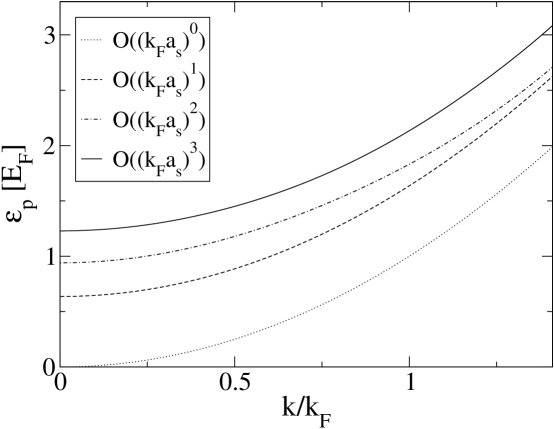
Figure 3: The quasiparticle energy $\epsilon_{p}$ in units of the Fermi energy $E_{F}$ up to order $(k_{F}/\Lambda)^{0}$ (dotted line), $(k_{F}/\Lambda)^{1}$ (dashed line), $(k_{F}/\Lambda)^{2}$ (dash-dotted line), and $(k_{F}/\Lambda)^{3}$ (solid line) for $k_{F}a_{s}=k_{F}a_{p}=k_{F}r_{s}=0.5$ and $g=4$.

As an example, we have chosen the parameters $k_{F}a_{s}=k_{F}a_{p}=k_{F}r_{s}=0.5$ and $g=4$. The width $\gamma_{k}$ shows the behavior predicted by the Lehmann representation, that is $\gamma_{k}>0$ for $k<k_{F}$ and $\gamma_{k}<0$ for $k>k_{F}$.

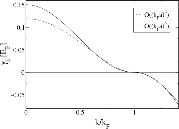
Figure 4: The quasiparticle width $\gamma_{p}$ in units of the Fermi energy $E_{F}$ up to order $(k_{F}/\Lambda)^{2}$ (dash-dotted line) and up to order $(k_{F}/\Lambda)^{3}$ (solid line) for $k_{F}a_{s}=k_{F}a_{p}=k_{F}r_{s}=0.5$ and $g=4$.

Our results agree qualitatively with the previous incomplete calculation of Bund and Wajntal bund where the particle-hole and effective range contributions were omitted. For those contributions for which a detailed comparison is possible, quantitative agreement is obtained as well.

Using Eqs. (28,30,31), we can immediately calculate the third order contributions to the above mentioned observables. As the effective mass $M^{*}$ is proportional to the inverse of the slope of the excitation energy at the Fermi surface, we need the complete result for $\epsilon_{k}$ up to order $(k_{F}/\Lambda)^{3}$:

$$\frac{M^{*}}{M} = \biggl{(}1+(g-1)\frac{8}{15\pi^{2}}(k_{F}a_{s})^{2}(1-7\log 2)+\frac{(g+1)}{3\pi}(k_{F}a_{p})^{3}+\frac{(k_{F}a_{s})^{2}k_{F}r_{s}}{6\pi}(g-1)$$ (32)

$$\qquad+0.11(g-1)(g-3)(k_{F}a_{s})^{3}-0.15(g-1)(k_{F}a_{s})^{3}\biggr{)}^{-1}$$

In order to check our calculation, we calculate the third order contribution to the chemical potential and the energy per particle. According to Eq. (24), the contribution to the chemical potential at ${\cal O}((k_{F}/\Lambda)^{3})$ is given by:

$$\mu_{(3)} = \frac{k_{F}^{2}}{2M}\biggl{[}(g-1)\frac{4}{15\pi}(k_{F}a_{s})^{2}k_{F}r_{s}+(g+1)\frac{8}{15\pi}(k_{F}a_{p})^{3}$$ (33)

$$\qquad+(g-1)\bigl{\{}0.20+(g-3)0.15\bigr{\}}(k_{F}a_{s})^{3}\biggr{]}~{}.$$

The third order contribution to the energy per particle is then given by:

$$\biggl{(}\frac{E}{N}\biggr{)}_{(3)} = \frac{k_{F}^{2}}{2M}\biggl{[}(g-1)\frac{1}{10\pi}(k_{F}a_{s})^{2}k_{F}r_{s}+(g+1)\frac{1}{5\pi}(k_{F}a_{p})^{3}$$ (34)

$$\quad+(g-1)\bigl{\{}0.076+(g-3)0.057\bigr{\}}(k_{F}a_{s})^{3}\biggr{]}~{},$$

which is in good agreement with previous results efimov ; baker ; bishop ; HAMMER00 .

Finally, we also calculate the wave function renormalization $Z$ defined in Eq. (21). It is related to the discontinuity in the momentum distribution at the Fermi surface Migdal57 . We obtain for $Z(k_{F})$:

$$Z(k_{F})^{-1} = 1-\frac{4(g-1)}{\pi^{2}}\log 2\,(k_{F}a_{s})^{2}$$ (35)

$$\qquad+\frac{8(g-1)}{\pi^{3}}\{0.184-(g-3)\,0.224\}(k_{F}a_{s})^{3}~{}.$$

We used the results of Sartor and Mahaux SARTOR80 for the occupation numbers to obtain an analytical expression for the second order term. We verified this result numerically. At third order, the results were computed numerically.

V Summary and Conclusions

In this paper, we have performed the first complete calculation of the the quasiparticle excitation energies and widths in the dilute Fermi gas to order $(k_{F}/\Lambda)^{3}$. In order to check our calculation, we have derived and compared the chemical potential and the energy per particle at $(k_{F}/\Lambda)^{3}$ to previous results.

The calculation has been carried out using an EFT for dilute Fermi systems HAMMER00 . Using dimensional regularization with minimal subtraction the power counting in this EFT is particularly simple. All loop momenta are converted to Fermi momenta which leads to a fully perturbative expansion. This is in contrast to previous calculations efimov ; baker ; bishop . There, a more general set of diagrams had to be first summed and then expanded with care to avoid double counting. The EFT approach is controlled and allows for systematic improvements by simply going to the next order in the power counting. Errors can be estimated reliably using dimensional analysis and error plots.

To order $(k_{F}/\Lambda)^{3}$ , no three-body input is required. At ${\cal O}((k_{F}/\Lambda)^{4})$, however, a contact three-body interaction enters. Without the three-body term, the logarithmic divergence appearing at this order can not be renormalized HAMMER00 . A complete calculation of the energy density to this order is in progress Luc02 .

The extension of the present EFT to the nuclear matter problem is not straightforward. The breakdown scale is set by the lowest momentum scale in the effective range expansion which is of order 10 MeV for nuclear matter because of the large S-wave scattering lengths. Similar problems arise for atomic systems near a Feshbach resonance. For scattering in the vacuum, the appropriate power counting to deal with the large scattering lengths is known vanKolck:1998bw ; ksw . It requires to sum all $C_{0}$ interactions which for two-particle nonrelativistic scattering simply involves summing a geometric series. At finite density, the diagrams involving only $C_{0}$ vertices are not easily summed because both particles and holes are present. To make the problem tractable, an additional ordering scheme such as the hole-line expansion in the standard nuclear physics approach is needed. Whether the hole-line expansion can be justified in EFT using power counting arguments remains to be seen. An interesting possibility is to exploit the geometry of intersecting Fermi spheres inherent in the finite density loop integrals which leads to an expansion in $1/D$ where $D$ is the space time dimension STEELE00 . Furthermore, an expansion in the inverse spin-isospin degeneracy $g=4$ might prove useful FURNSTAHL02 . The nuclear matter problem provides additional challenges. Since $k_{F}\approx 270$ MeV, the pion exchange is long range and cannot be treated within a purely short range EFT. Both the large scattering length problem and the inclusion of the long range pion exchange are important questions to be addressed by future work.

Recent progress in the field of cold Fermi gases jin99 ; hulet01 also opens the possibility of applications of EFT methods in the physics of cold fermionic atoms. In the case of cold bosons, EFT methods have already been applied successfully to a number of processes Bedaque:2000ft ; Braaten:2001hf ; Braaten:2001ay ; Bedaque:2002xy .

Appendix A Proper Self-Energy Integrals

We illustrate the calculation of the self-energy diagrams in Section III by applying the Feynman rules to diagram (7) from Fig. 2. This diagram has a symmetry factor of $1/4$. Thus, one obtains the following expression:

$$\Sigma^{*}_{3(7)}(\tilde{p})=(-iC_{0})^{3}\frac{i}{4}\frac{4(1-g)}{(2\pi)^{12}}\int\hbox{d}^{4}k\int\hbox{d}^{4}q\int\hbox{d}^{4}l\;i^{5}G_{0}(\tilde{k})G_{0}(\tilde{p}-\tilde{q})G_{0}(\tilde{k}+\tilde{q})G_{0}(\tilde{p}-\tilde{l})~{}.$$ (36)

After performing the contour integrations we have:

$$\Sigma^{*}_{3(7)}(\tilde{p}) = C_{0}^{3}\frac{g-1}{(2\pi)^{9}}\int\hbox{d}^{3}k\int\hbox{d}^{3}q\int\hbox{d}^{3}l$$

$$\Biggl{[}\frac{2\theta(k-k_{F})\theta(|\mathbf{k}+\mathbf{l}|-k_{F})\theta(|\mathbf{p}-\mathbf{l}|-k_{F})\theta(k_{F}-|\mathbf{k}+\mathbf{q}|)\theta(k_{F}-|\mathbf{p}-\mathbf{q}|)}{(p_{o}+\omega_{k}-\omega_{\mathbf{k}+\mathbf{q}}-\omega_{\mathbf{p}-\mathbf{q}}-i\epsilon)(\omega_{\mathbf{k}+\mathbf{q}}-\omega_{\mathbf{k}+\mathbf{l}}-\omega_{\mathbf{p}-\mathbf{l}}+\omega_{\mathbf{p}-\mathbf{q}}+i\epsilon)}$$

$$-\frac{\theta(k-k_{F})\theta(k_{F}-|\mathbf{k}+\mathbf{l}|)\theta(k_{F}-|\mathbf{p}-\mathbf{l}|)\theta(k_{F}-|\mathbf{k}+\mathbf{q}|)\theta(k_{F}-|\mathbf{p}-\mathbf{q}|)}{(p_{o}+\omega_{k}-\omega_{\mathbf{k}+\mathbf{l}}-\omega_{\mathbf{p}-\mathbf{l}}-i\epsilon)(p_{o}+\omega_{k}-\omega_{\mathbf{k}+\mathbf{q}}-\omega_{\mathbf{p}-\mathbf{q}}-i\epsilon)}$$

$$-\frac{2\theta(k_{F}-k)\theta(|\mathbf{k}+\mathbf{l}|-k_{F})\theta(|\mathbf{p}-\mathbf{l}|-k_{F})\theta(k_{F}-|\mathbf{k}+\mathbf{q}|)\theta(k_{F}-|\mathbf{p}-\mathbf{q}|)}{(p_{o}+\omega_{k}-\omega_{\mathbf{k}+\mathbf{l}}-\omega_{\mathbf{p}-\mathbf{l}}+i\epsilon)(\omega_{\mathbf{k}+\mathbf{l}}-\omega_{\mathbf{k}+\mathbf{q}}+\omega_{\mathbf{p}-\mathbf{l}}-\omega_{\mathbf{p}-\mathbf{q}}-i\epsilon)}$$

$$+\frac{\theta(k_{F}-k)\theta(|\mathbf{k}+\mathbf{l}|-k_{F})\theta(|\mathbf{p}-\mathbf{l}|-k_{F})\theta(|\mathbf{k}+\mathbf{q}|-k_{F})\theta(|\mathbf{p}-\mathbf{q}|-k_{F})}{(p_{o}+\omega_{k}-\omega_{\mathbf{k}+\mathbf{l}}-\omega_{\mathbf{p}-\mathbf{l}}+i\epsilon)(p_{o}+\omega_{k}-\omega_{\mathbf{k}+\mathbf{q}}-\omega_{\mathbf{p}-\mathbf{q}}+i\epsilon)}\Biggr{]}~{}.$$

By setting this expression on-shell (that is $p_{0}=p^{2}/(2M)$) and an appropriate substitution to dimensionless variables using

$$\mathbf{k}=k_{F}\mathbf{u},\quad\mathbf{q}=k_{F}\frac{1}{2}(\mathbf{v}-\mathbf{u}-2\mathbf{t}),\quad\mathbf{l}=k_{F}\frac{1}{2}(\mathbf{v}-\mathbf{u}-2\mathbf{r}),\quad\mathbf{p}=k_{F}\mathbf{v}~{},$$ (38)

Eq. (A) can be simplified significantly:

$$\Sigma^{*}_{3(7)}(\tilde{p}) = \frac{C_{0}^{3}M^{2}k_{F}^{5}(g-1)}{(2\pi)^{9}}\int\hbox{d}^{3}u\int\hbox{d}^{3}t\int\hbox{d}^{3}r$$

$$\Biggl{[}\frac{2\theta(u-1)\theta(|\mathbf{s}-\mathbf{r}|-1)\theta(|\mathbf{s}-\mathbf{r}|-1)\theta(1-|\mathbf{s}-\mathbf{t}|)\theta(1-|\mathbf{s}+\mathbf{t}|)}{(2q^{2}-2t^{2}-i\epsilon)(2t^{2}-2r^{2}-i\epsilon)}$$

$$-\frac{\theta(u-1)\theta(1-|\mathbf{s}-\mathbf{r}|)\theta(1-|\mathbf{s}-\mathbf{r}|)\theta(1-|\mathbf{s}-\mathbf{t}|)\theta(1-|\mathbf{s}+\mathbf{t}|)}{(2q^{2}-2r^{2}-i\epsilon)(2q^{2}-2t^{2}-i\epsilon)}$$

$$-\frac{2\theta(1-u)\theta(|\mathbf{s}-\mathbf{r}|-1)\theta(|\mathbf{s}-\mathbf{r}|-1)\theta(1-|\mathbf{s}-\mathbf{t}|)\theta(1-|\mathbf{s}+\mathbf{t}|)}{(2q^{2}-2r^{2}-i\epsilon)(2r^{2}-2t^{2}-i\epsilon)}$$

$$+\frac{\theta(1-u)\theta(|\mathbf{s}-\mathbf{r}|-1)\theta(|\mathbf{s}-\mathbf{r}|-1)\theta(|\mathbf{s}-\mathbf{t}|-1)\theta(|\mathbf{s}+\mathbf{t}|-1)}{(2q^{2}-2r^{2}+i\epsilon)(2q^{2}-2t^{2}+i\epsilon)}\Biggr{]}~{}.$$

We consider only the first term in the square brackets:

$$\mathcal{I}_{1}=\int\hbox{d}^{3}u\int\hbox{d}^{3}t\int\hbox{d}^{3}r\frac{2\theta(u-1)\theta(|\mathbf{s}-\mathbf{r}|-1)\theta(|\mathbf{s}-\mathbf{r}|-1)\theta(1-|\mathbf{s}-\mathbf{t}|)\theta(1-|\mathbf{s}+\mathbf{t}|)}{(2q^{2}-2t^{2}-i\epsilon)(2t^{2}-2r^{2}-i\epsilon)}~{},$$ (40)

where the constant overall prefactor in Eq. (A) has been dropped. By analyzing the step function, we can rewrite the integral as

$$\mathcal{I}_{1}=8\pi^{3}\int_{-1}^{1}\hbox{d}x\int_{1}^{\infty}\hbox{d}u\int_{0}^{1}\hbox{d}z\int_{0}^{z_{-}(s,z)}\hbox{d}t\int_{0}^{1}\hbox{d}y\int_{z_{+}(s,y)}^{\infty}\hbox{d}r\frac{u^{2}t^{2}r^{2}\theta(1-s)}{(q^{2}-t^{2}-i\epsilon)(t^{2}-r^{2}+i\epsilon)}~{},$$ (41)

with

$$z_{\pm}(s,z)=\pm sz+\sqrt{1-s^{2}(1-z^{2})}~{}.$$ (42)

The integral over $r$ contains a linearly divergent term which can be separated by writing

$$\int_{z_{+}(s,y)}^{\infty}\hbox{d}r\frac{r^{2}}{t^{2}-r^{2}+i\epsilon}=\int_{0}^{\infty}\hbox{d}r\frac{r^{2}}{t^{2}-r^{2}+i\epsilon}+\int_{0}^{z_{+}(s,y)}\hbox{d}r\frac{r^{2}}{t^{2}-r^{2}+i\epsilon}~{}.$$ (43)

The ultraviolet divergence is contained in the first term on the right-hand side of Eq. (43). In dimensional regularization with minimal subtraction the linear divergence is subtracted automatically and the finite part of this term is purely imaginary. Thus, we can write $\mathcal{I}_{1}$ as:

$$\mathcal{I}_{1} = 8\pi^{3}\int_{-1}^{1}\hbox{d}x\int_{1}^{\infty}\hbox{d}u\int_{0}^{1}\hbox{d}z\int_{0}^{z_{-}(s,z)}\hbox{d}t\quad\frac{u^{2}t^{2}\theta(1-s)}{(q^{2}-t^{2}-i\epsilon)}\biggl{(}-\frac{i\pi t}{2}\biggr{)}$$

$$-8\pi^{3}\int_{-1}^{1}\hbox{d}x\int_{1}^{\infty}\hbox{d}u\int_{0}^{1}\hbox{d}z\int_{0}^{z_{-}(s,z)}\hbox{d}t\int_{0}^{1}\hbox{d}y\int_{0}^{z_{+}(s,y)}\hbox{d}r\frac{u^{2}t^{2}r^{2}\theta(1-s)}{(q^{2}-t^{2}-i\epsilon)(t^{2}-r^{2}+i\epsilon)}~{}.$$

Separating the real and imaginary part of this integral and some further straightforward manipulations lead to expressions that can be integrated numerically. The remaining terms in the square brackets in Eq. (A) are treated analogously.

References

• (1) S. Weinberg, Physica 96A (1979) 327.
• (2) G.P. Lepage, “What is Renormalization?”, in From Actions to Answers (TASI-89), edited by T. DeGrand and D. Toussaint (World Scientific, Singapore, 1989); arXiv:nucl-th/9706029.
• (3) D.B. Kaplan, arXiv:nucl-th/9506035.
• (4) J. Gasser and H. Leutwyler, Nucl. Phys. B 250 (1985) 465.
• (5) U.-G. Meißner,“Chiral QCD: Baryon Dynamics”, in At the Frontier of Particle Physics, vol. 1, ed. M. Shifman (World Scientific, 2001) [arXiv:hep-ph/0007092]; V. Bernard, N. Kaiser, and U.-G. Meißner, Int. J. Mod. Phys. E 4 (1995) 193.
• (6) S.R. Beane, P.F. Bedaque, W.C. Haxton, D.R. Phillips, and M.J. Savage, “From Hadrons to Nuclei: Crossing the Border”, in At the Frontier of Particle Physics, vol. 1, ed. M. Shifman (World Scientific, 2001) [arXiv:nucl-th/0008064].
• (7) P.F. Bedaque and U. van Kolck, arXiv:nucl-th/0203055.
• (8) J.W. Negele and H. Orland, Quantum Many-Particle Systems (Addison-Wesley, New York, 1988).
• (9) A.L. Fetter and J.D. Walecka, Quantum Theory of Many-Particle Systems (McGraw–Hill, New York, 1971).
• (10) L.D. Landau, Sov. Phys. JETP 3 (1956) 920; 5 (1957) 101; 8 (1959) 70.
• (11) P. Nozieres, Theory of Interacting Fermi Systems, (Addison Wesley, Reading, 1997).
• (12) V.N. Efimov and M.Y. Amusia, Ann. Phys. (NY) 47 (1968) 377.
• (13) G.A. Baker, Phys. Rev. 140 (1965) B9; Rev. Mod. Phys. 43 (1971) 479.
• (14) R.F. Bishop, Ann. Phys. (NY) 77 (1973) 106.
• (15) H.-W. Hammer and R.J. Furnstahl, Nucl. Phys. A 678 (2000) 277, [arXiv:nucl-th/0004043].
• (16) B. DeMarco and D.S. Jin, Science 285 (1999) 1703.
• (17) A.G. Truscott, K.E. Strecker, W.I. McAlexander, G.B. Partridge, and R.G. Hulet, Science 291 (2001) 2570.
• (18) V.M. Galitskii, Sov. Phys. JETP 34 (1958) 104.
• (19) G.W. Bund and W. Wajntal, Nuovo Cimento 27 (1963) 1019.
• (20) R. Sartor and C. Mahaux, Phys. Rev. C 21 (1980) 1546.
• (21) J.M. Luttinger, Phys. Rev. 121 (1961) 942.
• (22) G.P. Lepage, J. Comp. Phys. 27 (1978) 192.
• (23) A.B. Migdal, Sov. Phys. JETP 5 (1957) 333.
• (24) R.J. Furnstahl and H.-W. Hammer, Phys. Lett. B 531 (2002) 203.
• (25) L. Platter, H.-W. Hammer, and U.-G. Meißner, in progress.
• (26) U. van Kolck, Nucl. Phys. A 645, 273 (1999).
• (27) D.B. Kaplan, M.J. Savage, and M.B. Wise, Nucl. Phys. B 534, 329 (1998).
• (28) J.V. Steele, arXiv:nucl-th/0010066.
• (29) R.J. Furnstahl and H.-W. Hammer, in preparation.
• (30) P.F. Bedaque, E. Braaten, and H.-W. Hammer, Phys. Rev. Lett.  85, 908 (2000).
• (31) E. Braaten and H.-W. Hammer, Phys. Rev. Lett.  87, 160407 (2001).
• (32) E. Braaten, H.-W. Hammer, and T. Mehen, Phys. Rev. Lett.  88, 040401 (2002).
• (33) P.F. Bedaque and G. Rupak, arXiv:cond-mat/0206527.