Scalar ground-state observables in the random phase approximation
Abstract
We calculate the ground-state expectation value of scalar observables in the matrix formulation of the random phase approximation (RPA). Our expression, derived using the quasiboson approximation, is a straightforward generalization of the RPA correlation energy. We test the reliability of our expression by comparing against full diagonalization in shell-model spaces. In general the RPA values are an improvement over mean-field (Hartree-Fock) results, but are not always consistent with shell-model results. We also consider exact symmetries broken in the mean-field state and whether or not they are restored in RPA.
pacs:
21.60.Jz,21.60.Cs,21.10.Ft,21.10.HwI introduction
Mean-field theory is the starting point for most microscopic models of many-body systems such as nuclei. In fact, for global studies of nuclear properties, such as nuclear binding energies, mean-field theory in the form of Hartree-Fock (HF) and related approximations are still the only viable microscopic approach HFmass ; otherwise one turns to semiclassical methods such as liquid drop MN95 and Thomas-Fermi AP95 .
Unfortunately, mean-field theory ignores particle-hole correlations and can break fundamental symmetries such as rotational and translational invariance. The next logical step beyond the static mean-field is known as the random phase approximation, or RPA, which can be derived in the small amplitude limit of time-dependent mean-field theory, and which implicitly allows for small correlations in the ground state Rowe70 ; ring ; BB .
The main applications of RPA have been to transition strengths and excitation spectra. One can also calculate the correction to the ground state energy due to RPA correlations, which was the basis of a recent proposal to use mean-field + RPA to compute global binding energy systematics bertsch2000 .
There are other potential quantities of interest, namely the ground state expectation value of observables other than the Hamiltonian. An important application is the root-mean-square radius. Any global fit of nuclear systematics involves both binding energies and nuclear radii. Indeed, most global fits to binding energies and radii with nonrelativistic phenomenological interactions such as Skyrme require density-dependent forces, although we will not deal specifically with that issue in this paper. Further challenges to mean-field calculations are isotopic shifts in the charge radius pa73 , and parity-violating electron scattering, which is sensitive to the difference between the neutron and proton rms radii pvrms .
In section II of this paper we present an expression for the ground-state expectation value of a general observable in RPA. This expression is derived using the quasiboson approximation, in exact analogy with the RPA correlation energy, and is a generalization of the RPA one-particle density derived by Rowe Rowe70 ; ro68 . Because the RPA ground state is approximated by a quasiboson vacuum, one can read off directly the expectation value without having to construct an explicit wavefunction.
Having an expression is not sufficient. Does it produce useful and reliable results? After all, RPA is an approximation, and because it violates the Pauli exclusion principle RPA is not even variational. Despite this, rigorous tests of the accuracy of RPA calculations have been spotty. For example, although the RPA correlation energy has been in the literature for decades, the only tests were in toy models toyrpa . Recently we compared the RPA correlation energy against exact shell-model results stetcu2002 . We found that generally RPA gave very good agreement–albeit with some significant failures which reduce the reliability of RPA binding energies.
We continue this program by computing the ground-state expectation value of observables both in exact shell-model calculations and in RPA. As discussed below, in this paper we limit ourselves to scalar operators. Unfortunately in harmonic oscillator model spaces is trivial, so we instead compute and compare the expectation values of a one-body operator: the number of particles outside the orbit; and several two-body operators: , , , and the pairing Hamiltonian .
The results are found in Section III. In general, RPA offers an improvement over the mean-field (HF) expectation values. This is not always the case, however, and even when HF+RPA is closer to the exact shell-model results than HF values, the improved agreement is sometimes still unsatisfactory. (The situation is reminiscent of variational calculations, where one typically gets much better agreement in energy than in the wavefunction. But again, RPA is not a variational theory.)
In section IV we turn to another issue of relevance to RPA: the restoration of symmetries, such as rotational invariance, broken by the mean field. We compute the expectation value of and compare the exact shell-model result against the Hartree-Fock and RPA values. If RPA “restores” the broken symmetry then one expects that either one regains the correct ground state value of or gets a much better value than the Hartree-Fock value. We find that, although often is improved by RPA corrections, one does not always regain a very good estimate of the ground state angular momentum. We interpret this to mean that RPA only approximately restores broken symmetries.
Nonetheless, we consider our results relevant. The RPA is not new, but we remind the reader that for global approaches to nuclear structure the state of the art is still mean-field theory; ab initio methods can only be applied to very light nuclei, and shell model diagonalization can only be applied piecewise. Consistent calculations using HF+RPA throughout the nuclides is conceiveable, however, and this paper is part of a larger program to rigorously test the reliability of RPA as an approximation to much larger microscopic calculations.
II corrections to a general operator in RPA
Before we derive the expectation value of an operator in RPA, we first begin with a brief pedagogical review of the derivation of the RPA correlation energy, including proper treatment of zero modes that correspond to broken symmetries. The RPA expectation value of a general operator then follows naturally.
There are many ways to derive RPA ring ; BB . One approach is to expand the energy about the Hartree-Fock miminum. Let be the Hartree-Fock Slater determinant, and let be small perturbations from the Hartree-Fock state. We follow the usual convention where denote single-particle states above the Fermi surface in the Hartree-Fock state, or “particle” states, while denote “hole” states below the Fermi surface. Then one can expand the energy surface in the vicinity of the Hartree-Fock minimum in terms of the particle-hole amplitudes up to second order:
| (1) |
where
| (2) | |||
| (3) |
We restrict ourselves to real wavefunctions, so that A, B are also real. There is no linear term in (1) because by the definition of the Hartree-Fock state. This quadratic surface can be mapped to a harmonic oscillator, replacing the by boson operators
| (4) |
which has analogous commutation relations, e.g., , etc. The boson Hamiltonian can be written in matrix form, which induces an additional constant term:
| (5) |
We want to put (5) into diagonal form, the first step of which is to solve the well-known RPA matrix equation:
| (6) |
The solutions have normalization .
Before going on one must treat carefully the case of zero modes, . Zero modes arise in RPA when an exact symmetry is broken. Suppose the HF state is deformed. The HF energy will not change as the orientation is rotated; this invariance is reflected in and resurfaces as RPA zero modes. (This is also a good check of one’s RPA codes. One expects three zero-frequency modes for triaxially deformed states, and two zero modes for an axisymmetric deformed state: rotation about an axis of symmetry takes one to the same, indistiguishable state.) One cannot define properly normalized for zero modes. Instead one introduces collective coordinates and conjugate momenta ring ; Rowe70 ; weneser , which satisfy
| (7) |
Here is a constant, interpretable as mass or moment of inertia but whose value depends on the normalization of , which are only constrained by
| (8) |
Now one obtains a generalized Bogoliubov transformation of the boson operators , , not only to quasibosons , , but also to the zero-mode collective coordinate operator and conjugate momentum operator :
| (9) | |||
Application of (9) and its Hermitian conjugate to (5) puts it in diagonal form:
| (10) |
The ground state is the quasiboson vacuum, and one can easily read off the RPA ground state energy, which is just the zero-point energy:
| (11) |
One can expand
| (12) |
where the second term is restricted to zero modes, and then obtain an expression equivalent to (11),
| (13) |
an expression which explicitly segregates out the contribution from zero modes.
The above derivation of the RPA correlation energy is well-known. We derive the RPA expectation value of any generator operator in exactly analogous fashion. Define , as in Eqs. (2) and (3), respectively, by replacing the Hamiltonian by the observable , that is,
| (14) | |||
| (15) |
and define , which does not in general vanish. (Because we restrict the Hartree-Fock state to real Slater determinants, and are real.) Please note that in computing , , and one still uses the Hartree-Fock state from minimizing the Hamiltonian , not from minimizing ; we are finding the expectation value in the vicinity of the minimum of .
The form of the operator in the harmonic oscillator bosons is
| (19) | |||
| (25) |
By transforming to the collective quasibosons (9), we again can trivially read off the quasiboson vacuum expectation value, which is the RPA ground-state expectation value, without explicit construction of a wavefunction:
| (26) |
where
| (27) |
Substitution of Eq. (6) with , derived from the Hamiltonian immediately regains the RPA binding energy (11). It is important to emphasize again that the , used here are those calculated from Eq. (6) using the original , matrices (from the Hamiltonian); one does not compute , using , .
As before we can rewrite (26) into an expression with explicit segregation of the zero modes:
| (28) | |||||
We have confirmed numerically that (28) yields the same values as (26).
As we will see in the next section, Eq. (26) reduces to that derived by Rowe for one-particle densities in spherical nuclei Rowe70 ; ro68 .
If is a scalar, so that it is invariant under rotation, translation, etc., then the above is sufficient. Nonscalar observables require a little more thought. In particular, consider observables that are angular momentum tensors, , with a nonzero rank . Here is the magnetic quantum number. If one applies the generalized Bogoliubov transformation (9) then the linear terms in do not vanish. The linear terms proportional to the quasiboson operators , are transitions to excited states; but, for nonscalars, there will be terms also proportional to and to . Furthermore, there will be quadratic terms, such as , , etc., which manifestly do not contribute to the ground state, but also terms quadratic in , . These terms arise from rotations (and in the more general case, translations, etc.): because they correspond to zero-frequency modes, they connect only to the ground state, but in a different orientation. If is a spherical tensor, we know how it transforms under a rotation, and the linear and quadratic terms in , etc., are simply the linear and quadratic terms for small rotation angles. Nonetheless, the issue of nonscalar observables is not trivial, and we leave it to future work.
To summarize a first result of the present work, we have extended the usual expansion of the Hamiltonian operator in the neighborhood of the HF solution to any operator, with the purpose to incorporate RPA correlations in computation of expectation values of relevant observables. In the next section we test the reliability of this formula in a non-trivial model, that is, the shell-model restricted space using realistic Hamiltonians.
III RPA vs. shell-model for scalar observables
In this section we test the RPA expectation value found in Eqs. (26), (28), against an exact numerical solution computed by diagonalizing a Hamiltonian in a shell-model basis. We work in complete spaces where the valence particles are restricted to the single-particle states of a single major harmonic oscillator shell, e.g., -- for sd or --- for pf shell. The cores are inert, 16O for the sd and 40Ca for the pf shell. In the the valence space we use realistic interactions: Wildenthal “USD” in the sd shell wildenthal and the monopole-modified Kuo-Brown “KB3” in the pf shell KB3 .
As mentioned in the introduction, an operator one would like to measure is . Unfortunately in a shell-model space is trivial. The operator has two pieces, a one-body piece , which has a constant expectation value in a single major harmonic oscillator shell, and a two-body piece ; but because is an odd-parity operator, the two-body piece is non-zero only across major shells. Therefore in this paper we consider other one- and two-body operators.
III.1 One-body operators
Using the quasiboson approximation, Rowe derived the RPA one-particle densities for spherical nuclei Rowe70 ; ro68 ; related formulas have been used to compute the isotope shift in calcium pa73 , ignoring the two-body contribution. Let be the number of particles excited above the Fermi surface into the particle state . ( is not a magnetic quantum number.) Here and from (28)
| (29) |
which is Rowe’s result for spherical Hartree-Fock states. If the HF state is deformed, however, one has to take into account zero modes. The second term in (28) can be simplified if one sums over all particle states , that is, the total number of particles excited above the Fermi surface; in that case one can use Eq. (8) and find
| (30) |
where is the number of zero modes, for an axisymmetric Hartree-Fock state, such as for 20Ne, and =3 for a triaxial state, found for 24Mg. We find often leads to negative occupation numbers! Note, however, that is not an angular momentum scalar, nor even a spherical tensor of fixed rank, for deformed states.
Instead we considered the only scalar one-body operators in our system, the occupation numbers of a -shell. Table 1 tabulates the Hartree-Fock, RPA, and exact shell-model (SM) values of . The results are rather poor, except for three cases with spherical Hartree-Fock states, 22O, 24O, and 48Ca (for which we instead tabulate ). 21O is weakly deformed and also shows a reasonable, albeit imperfect, improvement as one goes from the Hartree-Fock value to the RPA value.
| Nucleus | HF | RPA | SM |
|---|---|---|---|
| 20Ne | 1.60 | 1.75 | 1.60 |
| 22Ne | 1.49 | 1.64 | 1.47 |
| 24Mg | 2.13 | 1.85 | 2.31 |
| 28Si | 3.87 | 3.77 | 3.15 |
| 20O | 0.24 | 0.46 | 0.54 |
| 21O | 0.06 | 0.53 | 0.38 |
| 22O∗ | 0.00 | 0.67 | 0.54 |
| 24O∗ | 2.00 | 2.50 | 2.25 |
| 48Ca∗† | 8.00 | 7.73 | 7.78 |
| 22Na | 1.51 | 1.69 | 1.52 |
| 26Al | 2.29 | 2.51 | 2.18 |
| 19F | 1.02 | 1.10 | 1.52 |
| 21F | 0.84 | 0.56 | 0.87 |
| 25Mg | 2.21 | 3.09 | 1.96 |
To explore this issue further, we took 28Si and lowered the single-particle energy; eventually the Hartree-Fock state changes from deformed to spherical. The results are plotted in Figure 1. Again we see reasonable agreement for the spherical region, but poor agreement in the deformed regime.
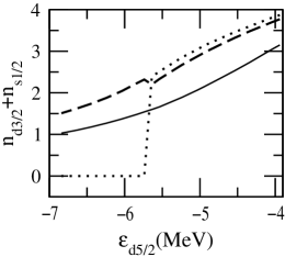
To summarize our results for one-body operators: we regain, for spherical Hartree-Fock states, Rowe’s one-particle occupation numbers and get improved values over the Hartree-Fock occupation numbers. For deformed nuclides, however, the RPA value is generally worse than the HF value. The fault does not appear to lie in the corrections due to zero modes; in the next section, we will find that the RPA expectation value of is more accurate in the deformed regime than in the spherical regime.
III.2 Two-body operators
We now turn to two-body operators, or more properly operators with both one- and two-body pieces. (We investigated the pure two-body pieces but found no qualitative differences; the pure two-body pieces performed neither better nor worse on the whole than the one-body pieces, which here are linear combinations of number operators.)
In Table 2 we show results for (total spin) and (total orbital angular momentum). The RPA expectation value is generally a significant improvement over the Hartree-Fock value, relative to the exact result. On the other hand, the RPA values, while closer to the mark, are not in very good agreement with the exact shell-model values, and sometimes overcorrect to negative, nonphysical expectation values (this can happen because RPA does not respect the Pauli exclusion principle).
In Table 3 we consider the expectation value of the pairing interaction, where , and of . We also show the ratio of correlation energies stetcu2002 which is a measure of how well the RPA binding energy tracks the exact binding energy. There appears to be no correspondence: a good RPA value for the binding energy does not correspond to a good RPA expectation value. In particular, note the single-species (oxygen) results, where the RPA binding energy is particularly bad; yet for these nuclides and are very good.
| Nucleus | |||||||
|---|---|---|---|---|---|---|---|
| HF | RPA | SM | HF | RPA | SM | ||
| 20Ne | 0.35 | 0.33 | 0.26 | 15.90 | -0.25 | 0.26 | |
| 22Ne | 1.48 | 0.48 | 0.88 | 16.76 | 0.31 | 0.88 | |
| 24Mg | 1.39 | 1.38 | 1.03 | 20.65 | -1.17 | 1.03 | |
| 26Mg | 2.04 | 1.14 | 1.45 | 18.94 | -0.34 | 1.45 | |
| 28Si | 1.62 | 1.28 | 1.45 | 21.50 | -0.75 | 1.45 | |
| 44Ti | 1.03 | 0.75 | 0.64 | 30.34 | -2.48 | 0.64 | |
| 46Ti | 2.24 | 1.20 | 1.36 | 29.72 | -2.94 | 1.36 | |
| 48Cr | 3.12 | 0.99 | 1.70 | 29.77 | 5.38 | 1.70 | |
| 20O | 1.50 | 0.45 | 0.75 | 6.80 | 0.92 | 0.75 | |
| 22O | 2.40 | -0.15 | 1.26 | 2.40 | 6.36 | 1.26 | |
| 24O | 2.40 | -0.27 | 1.29 | 2.39 | 6.06 | 1.29 | |
| 20F | 2.00 | 1.44 | 1.74 | 14.21 | 8.09 | 3.55 | |
| 22Na | 2.20 | 1.90 | 2.14 | 21.32 | 9.08 | 8.07 | |
| 26Al | 3.14 | 1.96 | 1.45 | 29.56 | 20.14 | 1.45 | |
| 46V | 2.51 | 1.50 | 1.36 | 35.39 | 16.33 | 1.36 | |
| 19F | 1.09 | 0.80 | 0.87 | 12.61 | 4.39 | 0.22 | |
| 21F | 2.11 | 0.76 | 1.52 | 13.31 | 5.60 | 6.41 | |
| 21Ne | 1.11 | 0.44 | 1.00 | 17.55 | 10.11 | 3.22 | |
| 23Na | 2.02 | 0.88 | 1.15 | 18.81 | 7.46 | 3.93 | |
| 25Mg | 2.04 | 0.38 | 1.73 | 22.56 | 11.77 | 7.68 | |
| Nucleus | Pairing | ||||||
|---|---|---|---|---|---|---|---|
| HF | RPA | SM | HF | RPA | SM | ||
| 20Ne | 2.99 | 5.47 | 6.81 | 715 | 825 | 793 | 0.75 |
| 22Ne | 3.99 | 7.25 | 9.31 | 876 | 1007 | 944 | 0.97 |
| 24Mg | 5.99 | 10.14 | 11.72 | 1167 | 1263 | 1268 | 0.92 |
| 26Mg | 6.99 | 11.51 | 14.56 | 1001 | 1104 | 1048 | 0.94 |
| 28Si | 8.99 | 12.73 | 15.16 | 1304 | 1389 | 1214 | 0.90 |
| 20O | 2.00 | 5.18 | 7.25 | 257 | 353 | 339 | 1.09 |
| 22O | 3.00 | 5.83 | 6.20 | 163 | 277 | 270 | 1.67 |
| 24O | 4.00 | 6.52 | 6.58 | 122 | 194 | 191 | 1.83 |
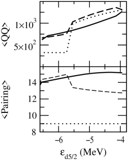
Again we look at the transition from deformed to spherical in 28Si for and , in Fig. 2, which clearly shows the RPA values are in better agreement in the spherical regime than in the deformed regime. (As it happens, of the nuclides we investigated 28Si, while convenient for comparing spherical vs deformed regimes, is the only nuclide for which the RPA value of is worse than the HF value, using the original Wildenthal single-particle energies.) This is not universal behavior; as seen in Table 2 and will be seen in the next section for , the RPA expectation value for some operators is better in the deformed regime.
IV Restoration of broken symmetries?
The random phase approximation respects broken symmetries by separating out exactly, as zero modes, spurious motion. This is sometimes interpreted as an “approximate restoration of the symmetry” ring . The restoration cannot be exact, because the RPA wavefunction is valid only in the vicinity of the Hartree-Fock state weneser and cannot be extrapolated to, for example, large rotation angles.
Still, we now have a tool to further explore symmetry restoration, by computing Casimir operators of symmetry groups. Specificially, we consider . Ideally, if the RPA restores a broken symmetry, one might imagine that one either regains the exact ground state value of or gets very close to it.
We present our results in Table 4. The pattern is the same as with other operators: is generally better in RPA than in Hartree-Fock but not always very close to the exact shell-model value. Even worse are the cases with a closed shell in HF, such as 22,24O: the HF value is correct, while the RPA value is terrible!
| Nucleus | HF | RPA | SM |
| 20Ne | 16.06 | -0.45 | 0 |
| 22Ne | 17.17 | -1.16 | 0 |
| 24Mg | 20.13 | -2.52 | 0 |
| 26Mg | 18.61 | -1.72 | 0 |
| 28Si | 20.89 | -1.99 | 0 |
| 44Ti | 31.65 | -3.10 | 0 |
| 46Ti | 31.53 | -5.00 | 0 |
| 48Cr | 29.37 | 4.72 | 0 |
| 20O | 6.07 | 1.76 | 0 |
| 22O | 0.00 | 7.99 | 0 |
| 24O | 0.00 | 7.38 | 0 |
| 20F | 18.46 | 12.41 | 6 |
| 22Na | 25.57 | 14.57 | 12 |
| 26Al | 35.98 | 27.92 | 0 |
| 46V | 39.56 | 20.00 | 0 |
| 19F | 15.12 | 5.52 | 0.75 |
| 21F | 15.51 | 9.47 | 8.75 |
| 21Ne | 19.05 | 12.68 | 3.75 |
| 23Na | 19.42 | 11.87 | 3.75 |
| 25Mg | 23.87 | 14.51 | 8.75 |
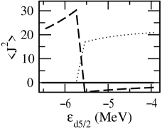
To examine this issue more closely, in Fig. 3 we again plot, for 28Si, versus the single-particle energy through the transition from deformed to spherical HF state. The results are better for the deformed HF state, although we obtain slightly negative, and thus nonphysical, values of .
An additional test of symmetry restoration would be computation of the expectation value of a nonscalar observable, such as the magnetic dipole moment or electric quadrupole moment, for a deformed nucleus with a shell-model ground state. We have preliminary, unpublished calculations which suggest that indeed the RPA ground state of even-even nuclides retains a significant quadrupole moment, another piece of evidence that symmetry is incompletely restored.
There are other observables one would like to compute relevant to broken symmetries. Aside from the Casimir itself, the dispersion of a Casimir would be a useful measure. For example, consider quasi-particle RPA (QRPA), where particle number is broken in the Hartree-Fock-Bogoliubov state. One would like to see the QRPA value of the dispersion move close to zero. Another example would be proton-neutron RPA (pnRPA) or pnQRPA, allowing protons and neutrons to mix, so that is no longer an good quantum number; this is applicable to beta decay. Here one might consider . Unfortunately, we suspect that the dispersion would also signal incomplete symmetry restoration.
V Summary and conclusion
We derived a expression for the ground-state expectation value of observables in the matrix formulation of RPA, and tested it against exact shell-model calculations for selected scalar operators. The RPA value was in general an improvement over the Hartree-Fock value, but failed to be a consistent and reliable estimate of the exact expectation value. Nonetheless this work should be considered a starting point for any modified RPA calculations, such as renormalized RPA, etc.
In particular we considered the expectation value of . If one starts with a deformed Hartree-Fock state, which breaks rotational invariance, the RPA approximately restores rotational symmetry, as evinced by better values of The results are not wholly satisfactory, however, as can take on unphysical (negative) values; furthermore, if one starts from a Hartree-Fock state with good symmetry, the HF value of is correct while the RPA value is large and positive, a disappointing result. Thus, while the RPA respects or identifies broken symmetries exactly, one can only characterize the restoration of symmetry in the RPA as approximate and somewhat unreliable.
Acknowledgements.
The U.S. Department of Energy supported this investigation through grant DE-FG02-96ER40985.References
- (1) F. Tondeur, S. Goriely, J.M. Pearson, and M. Onsi, Phys. Rev. C 62, 024308 (2000).
- (2) P. Möller, J.R. Nix, W.D. Myers, and W.J. Swiatecki, At. Data Nucl. Data Tables 59, 185 (1995).
- (3) Y. Aboussir, J.M. Pearson, A.K. Dutta, and F. Tondeur, At. Data Nucl. Data Tables 61, 127 (1995).
- (4) D. J. Rowe, Nuclear Collective Motion, Methuen and Co. Ltd., London 1970.
- (5) P. Ring and P. Shuck, The Nuclear Many-Body Problem, 1st edition, Springer-Verlag, New York 1980.
- (6) G. F. Bertsch and R. A. Broglia, Oscillations in Finite Quantum Sytems, Cambridge University Press, Cambridge, 1994
- (7) G.F. Bertsch and K. Hagino, Yad. Fiz. 64, 646 (2001) [Phys. Atom. Nucl. 64, 588 (2001)] preprint arXiv: nucl-th/0006032].
- (8) J. K. Parikh, Phys. Rev. C 8, 1433 (1973); E. Tinková and M. Gmitro, Phys. Rev. C 14, 1213 (1976).
- (9) C. J. Horowitz, S. J. Pollock, P. A. Souder, and R. Michaels Phys. Rev. C 63, 025501 (2001); D. Vretenar, P. Finelli, A. Ventura, G. A. Lalazissis, and P. Ring, Phys. Rev. C 61, 064307 (2000); B. Q. Chen and P. Vogel, Phys. Rev. C 48, 1392 (1993); S. J. Pollock, E. N. Fortson, and L. Wilets, Phys. Rev. C 46, 2587 (1992).
- (10) D. J. Rowe, Phys. Rev. 175, 1283 (1968).
- (11) K. Hagino and G.F. Bertsch, Phys. Rev. C61 024307 (2000); K. Hagino and G.F. Bertsch, Nucl. Phys. A679 163 (2000); N. Ullah and D.J. Rowe, Phys. Rev. 188, 1640 (1969); J.C. Parikh and D.J. Rowe, Phys. Rev. 175, 1293 (1968).
- (12) I. Stetcu and C.W. Johnson, accepted for publication in Phys. Rev. C; preprint arXiv:nucl-th/0205029.
- (13) E. R. Marshalek and J. Weneser, Ann. Phys. 53, 569 (1969).
- (14) B.H. Wildenthal, Prog. Part. Nucl. Phys. 11, 5 (1984).
- (15) T.T.S. Kuo and G.E. Brown, Nucl. Phys. A114, 235 (1968); A. Poves and A.P. Zuker, Phys. Rep. 70, 235 (1981).