Negative heat capacities and first order phase transitions in nuclei

Abstract

Anomalous negative heat capacities have been claimed as indicators of first order phase transitions in finite systems in general, and for nuclear systems in particular.  A thermodynamic approach allowing for all $Q$ value terms is used to evaluate heat capacities in finite van der Waals fluids and finite lattice systems in the coexistence region. Fictitious large effects and negative heat capacities are observed in lattice systems when periodic boundary conditions are introduced.  Small anomalous effects are predicted for small drops and for finite lattice systems.  A straightforward application of the analysis to nuclei shows that negative heat capacities cannot be observed for $A>60$.

The quest for discovery of the liquid to vapor phase transition in nuclei has progressed along two lines.  On one hand, the cluster abundance has been studied as a function of mass and temperature and the phase diagram has been generated [1] in terms of Fisher’s theory of clusterization [2].  On the other, caloric curves have been analyzed to look for plateaus and breaks possibly associated with the phase transition [3]; and fluctuations have been translated into heat capacities in the hope of discovering negative values which are widely considered to be indicators of phase coexistence in small systems [4, 5].

Regarding experimental caloric curves, it has been pointed out that their interpretation hinges upon an unknown pressure-volume relationship in the experiment, e.g. constant pressure or constant volume [6, 7].

Regarding the heat capacities, negative values are typically obtained in lattice gas, Ising, or Potts model calculations for finite systems [8, 9, 10].  The origin of these negative values is generically attributed to the generation of surface with its attendant energy cost, which is significant in small systems and which disappears in the thermodynamic limit.  However, with numerical calculations, it is not clear how this effect actually comes about, and if and how it may apply to actual systems like nuclei.  The issue is all the more interesting since claims of negative heat capacities have been made for nuclear systems [4, 5].

In this paper we are going to investigate the subject of caloric curves and heat capacities of finite systems in the coexistence region and the underlying role of varying potential energies (“ground states”) with system size on the basis of simple and very general thermodynamical concepts, in the hope of obtaining solid and unambiguous conclusions on these matters.

Our study applies to leptodermous (thin skinned) van der Waals-like fluids and to models such as Ising, Potts, and lattice gas, which are capable of reproducing their general features.  We shall show that:

1. drops of leptodermous systems can indeed show negative heat capacities as a slight effect if allowed to evaporate at constant pressure;

2. finite lattice systems can also present negative heat capacities as a slight effect if open boundary conditions are applied;

3. finite lattices systems present negative heat capacities as a much greater effect if periodic boundary conditions are applied, the main signal being associated with the latter, very artificial conditions;

4. nuclei cannot show negative heat capacities above $A\approx 60$, while negative heat capacities are possible for $A$ values below $60$.

Let us consider a macroscopic drop of a van der Waals fluid with $A$ constituents in equilibrium with its vapor.  The vapor pressure $p$ at temperature $T$ is given by the Clapeyron equation

$$\frac{dp}{dT}=\frac{\Delta H_{m}}{T\Delta V_{m}}$$ (1)

where $\Delta H_{m}$ is the molar vaporization enthalpy and $\Delta V_{m}$ is the molar change in volume.  The Clapeyron equation gives a direct connection between what we might call the “ground state” properties of the system and the saturation pressure along the coexistence line.  In fact, we can write

$$\Delta H_{m}=\Delta E_{m}+P\Delta V_{m}\sim\Delta E_{m}+T$$ (2)

and for $T\ll\Delta E$, $\Delta H_{m}\approx a_{v}$ can be identified approximately with the liquid-drop volume coefficient in the absence of other terms like surface and Coulomb, etc.  Assuming $\Delta V_{m}\approx V_{m}^{\text{vapor}}$, that the vapor is an ideal gas and that $\Delta H_{m}$ is constant with temperature, Eq. (1) can be integrated to give

$$p\simeq p_{o}\exp\left(-\frac{\Delta H_{m}}{T}\right).$$ (3)

Equation (3) represents the $p$-$T$ univariant line in the phase diagram of the system if $\Delta H_{m}$ is assigned its bulk value $\Delta H^{0}_{m}$.  It was observed long ago that for a drop of finite size $\Delta H_{m}$ must be corrected for the surface energy of the drop [11]

$$\Delta H_{m} = \Delta H_{m}^{0}+\Delta H_{m}^{s}=\Delta H_{m}^{0}-\gamma S_{m}$$ (4)

$$= \Delta H_{m}^{0}-a_{s}\frac{A^{2/3}}{A}=\Delta H_{m}^{0}-\frac{K}{r}$$ (5)

where $\gamma$ is the surface tension, $S_{m}$ is the molar surface of the drop of radius $r$, $a_{s}$ is the surface energy coefficient and $K$ is a geometrical constant.  Substitution in Eq. (3) leads to

$$p = p_{0}\exp\left(-\frac{\Delta H_{m}^{0}}{T}+\frac{a_{s}}{A^{1/3}T}\right)$$ (6)

$$= p_{\text{bulk}}\exp\left(\frac{a_{s}}{A^{1/3}T}\right)=p_{\text{bulk}}\exp\left(\frac{K}{rT}\right).$$ (7)

At constant temperature the vapor pressure increases with decreasing size of the drop.  In other words, each drop of constant radius $r$ has its own $r$-dependent coexistence line with the vapor as shown in Fig. 1.

FIG. 1.: The natural log of the saturated vapor pressure as a function of the inverse temperature for different droplet radii.  The size of the open circles is proportional to the droplet radius.  Arrows illustrate the path of evaporation at constant pressure.

Let us now consider the case of isobaric evaporation of a drop starting from a drop with $A_{0}$ constituents and evaporating into a drop with $A<A_{0}$ constituents.  Let us now define the drop size parameter

$$y=\frac{A_{0}-A}{A_{0}}.$$ (8)

At constant pressure

$$p_{0}\exp\left(-\frac{\Delta H_{m}^{0}}{T}\right)=p_{0}\exp\left(-\frac{\Delta H_{m}(y)}{T_{y}}\right).$$ (9)

Remembering that in most liquids $\left|a_{v}\right|\approx\left|a_{s}\right|$ and that in the lattice gas $\left|a_{v}\right|=\left|a_{s}\right|$, we have

$$\Delta H_{m}(y)\simeq a_{v}\left(1-\frac{1}{A_{0}^{1/3}(1-y)^{1/3}}\right)$$ (10)

from which follows

$$\frac{T_{y}}{T_{\infty}}\simeq\frac{\Delta H_{m}(y)}{\Delta H_{m}^{0}}\simeq 1-\frac{1}{A^{1/3}}\simeq 1-\frac{1}{A_{0}^{1/3}(1-y)^{1/3}}.$$ (11)

Thus, a slight decrease in temperature is predicted as the drop evaporates isobarically, thus leading to a negative isobaric heat capacity in the coexistence region as illustrated in Fig. 2.  In this figure, the abscissa is trivially related to $\Delta H$, the heat absorbed by the evaporating drop at constant pressure, by the relationship

$$\Delta H=A_{0}\int_{0}^{y}dy\Delta H_{m}(y)=A_{0}y\overline{\Delta H_{m}}.$$ (12)

The same decrease can be more visually appreciated from Fig. (1).  As the drop is evaporating at constant pressure, the drop moves from one coexistence curve to another according to its decrease in radius, and thus to progressively lower temperatures.  This slight effect is due not to an increase in surface as the drop evaporates, since the drop surface of course diminishes as $A^{2/3}$, but to the slight increase of molar surface which does increase as $A^{-1/3}$ as shown in Fig. 3.  Also, the formation of bubbles in the body of the drop is thermodynamically disfavored by the factor $f=\exp(-\gamma\Delta S/T)$ where $\Delta S$ is the surface of the bubble.

FIG. 2.: The temperature as a function of droplet size for a drop evaporating at constant pressure in a system with open boundary conditions.  The solid line shows the case of a spherical drop, while the dotted line shows the case of a finite cubic lattice evolving as in Fig. 3 top.

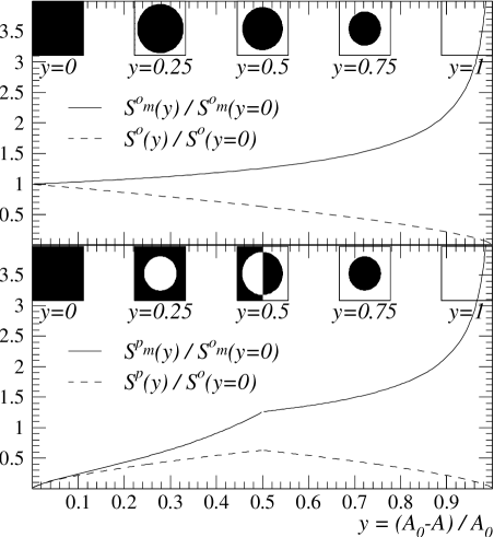
FIG. 3.: Top: The surface $S^{o}$ (dashed) and molar surface $S^{o}_{m}$ (solid) area of a drop for open boundary conditions normalized to their values at $y=0$.  Bottom: The surface $S^{p}$ (dashed) and molar surface $S^{p}_{m}$ (solid) area of a drop for periodic boundary conditions normalized to their values at $y=0$.  In-sets show the configurations at various values of $y$.

It is worth pointing out that the smallness of the effect ($\sim 4$% decrease in $T$ as a droplet of $A\sim 200$ evaporates all the way to $A\sim 100$), is needlessly magnified by the widely practiced artful translation of the caloric curve into heat capacity, which jumps from $+\infty$ to $-\infty$ as the slope of the caloric curve changes from constant to a slightly negative value.

It might be argued that cluster formation may be responsible for negative heat capacities.  In physical fluids as well as in the Ising model the “mean” molecular weight of the equilibrium vapor remains very close to that of the monomer, as confirmed by the adherence of the vapor pressure vs. temperature to the Clapeyron-Clausius formula with constant $\Delta H_{m}$ [12].  Furthermore, if such an effect existed it would operate already for the infinite systems, which, patently, it does not.

Let us now move to the amply studied cases of lattice gas, Ising, and Potts models.  Here as above, the study of the evolution of the ground state properties can be directly translated into the liquid-vapor coexistence properties.  We consider first an evaporating finite system in three dimensions of size $A_{0}=L^{3}$, with open boundary conditions.  This case is essentially identical to the case of a drop discussed above (see Fig. 2).

For maximal density at $T=0$ (the ground state) $y=0$ and the entire cubic lattice is filled.  For decreasing densities, always at $T=0$ a single cluster of minimum surface is present, which evolves from a cube to a sphere.  The associated change in surface is shown in Fig. (3).

Since a cube has only a slightly larger surface than a sphere of the same volume by a factor of $6/\left(\left(4\pi\right)^{1/3}3^{2/3}\right)$ the resulting decrease of $T_{y}$ at $y=1$ is nearly exactly what a sphere of the same volume would experience in going from $y=0$ to $y=1/2$ ($A_{0}\sim 200$).  Thus the caloric curve from $y=0$ to $y=1/2$ is essentially flat like in the infinite system, and the heat capacity is trivially infinite.

So, where are the large effects reported in so many papers [8, 9, 10]?  We shall see below the effect created by the introduction of periodic boundary conditions.

The introduction of periodic boundary conditions rids the system of “dangling bonds,” as it were, by repeating a cubic lattice of side $L$ periodically along the three coordinates.  These conditions, originally introduced to mimic the infinite system, lead here to peculiar consequences.

At $y=0$, the lattice is filled with particles so that $\Delta H_{m}(0)=\Delta H_{m}^{0}$ characteristic of the infinite system.  As $y$ increases at fixed lattice size, a bubble develops in the cube and surface is rapidly created.  This is shown in Fig. (3).  The bubble develops since the periodic boundary conditions prevent ’as it were’ evaporation from the surface.  The bubble grows with increasing $y$ until it touches the sides of the lattice.  This occurs for $y\approx 1/2$.  At nearly $y=1/2$ and beyond, the “stable” configuration is a drop that eventually vanishes at $y=1$.  The change in surface associated with the range $0\leq y\leq 1$ as well as the molar surface are shown in the bottom panel of Fig. 3.

FIG. 4.: The temperature as a function of droplet size for a drop evaporating at constant pressure in a system with periodic boundary conditions.  The solid line shows the case of a finite cubic lattice with periodic boundary conditions evolving as in Fig. 3 bottom, while the dotted line and the dashed line are the same as in Fig. 2 and the vertical dash-dotted line indicates the case of $50$% lattice occupation.

The evaporation enthalpy thus becomes

$$\Delta H_{m}(y)\simeq a_{v}\left(1-\frac{y^{2/3}}{A_{0}^{1/3}\left(1-y\right)}\right)$$ (13)

from $y=0$ to $y=1/2$, and

$$\Delta H_{m}(y)\simeq a_{v}\left(1-\frac{1}{A_{0}^{1/3}\left(1-y\right)^{1/3}}\right)$$ (14)

from $y=1/2$ to $y=1$.

As a consequence, for periodic boundary conditions

$$\frac{T_{y}}{T_{\infty}}\simeq 1-\frac{y^{2/3}}{A_{0}^{1/3}\left(1-y\right)}$$ (15)

from $y=0$ to $y=1/2$, while from $y=1/2$ to $y=1$ Eq. (11) holds.

The results contained in equations (11) and (15) are very general and convenient.  They bypass the clumsy numerical calculations for individual systems, and require, for any case, just the knowledge of the geometry and of the surface energy coefficient.

The dramatic effect of periodic boundary conditions can now be seen in Fig. 4.  The temperature decreases substantially with increasing $y$, due to the fact that the molar enthalpy at $y=0$ assumes its bulk value $\Delta H_{m}^{0}$ and must meet the previous case of open boundary conditions for $y=1/2$.  This may well explain the calculated negative heat capacities reported in literature, as an artifact due to the unnatural choice of boundary conditions.  The conclusion of this exercise is the following: if $\Delta H_{m}(y)$ decreases with $y$ (with decreasing drop size), for any reason, we expect negative heat capacities.  Alternatively we expect the normal infinite heat capacities if $\Delta H_{m}=$ constant or positive heat capacities if $\Delta H_{m}$ increases with $y$.

With the lessons learned above we can evaluate the heat capacities for nuclei.  It is apparent from the above arguments that the key quantity is $\Delta H_{m}$ and its dependence on the drop size, irrespective of the physical causes that determine its magnitude and dependence.  In the case of nuclei the quantity $\Delta H_{m}$ is determined not only by the volume and surface, but also by all the other terms in the liquid drop model, such as the Coulomb and symmetry energy all of which contribute to the mean binding energy per nucleon.  Consequently one can immediately infer that when the binding energy per nucleon decreases with $A$, the heat capacity should be positive, and vice-versa.  Thus, since the maximum binding energy per nucleon occurs at $A\sim 60$, negative heat capacities should be possible only for $A<60$.  Let us proceed more precisely.  We can rely again on the Clapeyron equations to calculate the heat capacity as follows

$$C_{p}=\left.\frac{dH}{dT}\right|_{p}=-\left.\frac{dH}{dA}\right|_{p}\left.\frac{dA}{dT}\right|_{p}=-\left.\Delta H_{m}(A)\frac{dA}{dT}\right|_{p}$$ (16)

but

$$\left.\frac{dT}{dA}\right|_{p}=\left.\frac{dp}{dA}\right|_{T}\left.\frac{dT}{dp}\right|_{p}.$$ (17)

From the integrated form of the Clapeyron equation we have

$$\left.\frac{dp}{dA}\right|_{p}=-\frac{1}{T}\frac{d\Delta H_{m}}{dA}p$$ (18)

so

$$\left.\frac{dT}{dA}\right|_{T}=-\frac{1}{T}\frac{d\Delta H_{m}}{dA}p\frac{TV_{m}}{\Delta H_{m}}=-\frac{T}{\Delta H_{m}}\frac{d\Delta H_{m}}{dA}.$$ (19)

Finally

$$C_{p}=\frac{\frac{\left(\Delta H_{m}(A)\right)^{2}}{T}}{\frac{d\Delta H_{m}}{dA}}.$$ (20)

The derivative in the denominator can be evaluated approximately from the dependence on the binding energy per nucleon $B$ upon the mass number

$$\frac{d\Delta H_{m}}{dA}=\frac{dB}{dA}.$$ (21)

The liquid drop model allows us to estimate such a derivative.  Without the Coulomb term, of course, we recover the results presented above for a drop: the binding energy increases with increasing $A$ and tends asymptotically to the value $a_{v}\approx 15$MeV.  Thus negative heat capacities should be expected and the caloric curves should look like that shown in Fig. 2.  The Coulomb and symmetry terms, however, become very important at large values of $A$, say, along the line of $\beta$-stability.  From Fig. 5 it is apparent that the binding energy decreases with $A$ for $A>\sim 60$.  Consequently in all this region of $A$, positive specific heats should be expected.  Only for $A<\sim 60$, negative specific heats are predicted.

FIG. 5.: Top: The binding energy per nucleon of atomic nuclei.  Bottom: The associated heat capacity.

Despite the assumption of a temperature independent $\Delta H_{m}$ we expect these results to hold over a very broad range of temperatures.  On one hand a monotonic change of $\Delta H_{m}$ with $T$ should not alter the result; on the other hand it is known that for van der Waals fluids their vapor pressure $p=p(T)$ is well defined up to the critical point by a constant $\Delta H_{m}$ [12].  Furthermore the appearance of clusters has minimal influence on $\Delta H_{m}$ and therefore on our results, because the vapor concentration is dominated by monomers [1].

This straightforward result based on elementary thermodynamics and ground state binding energies raises serious questions as to the meaning of the negative heat capacities that have been claimed for large nuclear systems.

In conclusion, we have shown that:

1. it is possible to generate caloric curves and heat capacities in the coexistence region from the knowledge of the molar heat of vaporization, which must include all $Q$-value terms;

2. simple drops and Ising, Potts models with open boundary conditions show minimal anomalies, while periodic boundary conditions introduce strong anomalies as artifacts;

3. nuclei with $A>\sim 60$ should present no anomalous negative heat capacities while this is possible for $A\leq\sim 60$.

This work was supported by the Director, Office of Energy Research, Office of High Energy and Nuclear Physics, Nuclear Physics Division of the US Department of Energy, under Contract No. DE-AC03-76SF00098.

REFERENCES

- [1] J. B. Elliott et al., Phys. Rev. Lett. 88, 042701 (2002).
- [2] M.E. Fisher, Physics 3, 255 (1967).
- [3] J. Pochodzalla et al., Phys. Rev. Lett. 75, 1040 (1995).
- [4] M. D’Agostino et al., Phys. Lett. B 473, 219 (2000).
- [5] M. D’Agostino et al., Nucl. Phys. A 699, 795 (2002).
- [6] L. G. Moretto et al., Phys. Rev. Lett. 76, 2282 (1996).
- [7] J. B. Elliott and A. S. Hirsch, Phys. Rev. C 61 054605 (2000).
- [8] T. L. Hill, J. Chem. Phys. 23, 812 (1955).
- [9] D. H. E. Gross, Phys. Rep. 279, 119 (1997).
- [10] Ph. Chomaz, et al., Phys. Rev. Lett. 85, 3587 (2000).
- [11] L. Rayleigh, Phil. Mag. 34, 94 (1917).
- [12] E.A. Guggenheim, “Thermodynamics”, th ed. (North-Holland, 1993).