A computer program for nuclear scattering at intermediate and high energies

Abstract

A computer program is presented which calculates the elastic and inelastic scattering in intermediate and high energy nuclear collisions. A coupled-channels method is used for Coulomb and nuclear excitations of E1, E2, E3, M1, and M2 multipolarities, respectively. The program applies to an arbitrary nucleus, specified by the spins and energies of the levels and by reduced matrix elements. For given bombarding conditions, the angular distribution of elastic and inelastic scattered particles and angular distributions of gamma-rays from the excited nucleus are computed.

I PROGRAM SUMMARY

1. Title of program: DWEIKO (Distorted Wave EIKOnal Approximation)

   Program obtainable from: CPC Program Library, Queen’s University of Belfast, N. Ireland

   Computers: The code has been created on an IBM-PC, but also runs on UNIX machines.

   Operating systems: WINDOWS or UNIX

   Program language used: Fortran-77

   Memory required to execute with typical data: 8 Mbytes of RAM memory and 1 MB of hard disk space

   No. of bits in a word: 64

   Memory required for test run with typical data: 1 MB

   No. of bytes in distributed program, including test data, etc.: 82238

   Distribution format: ASCII

   Keywords: Elastic scattering; Coulomb excitation; Relativistic collisions; Coupled-channels; Nuclear excitation

   Nature of physical problem: The program calculates elastic scattering differential cross sections, probabilities, and cross sections for inelastic scattering in nuclear collisions at intermediate and high energies ($E_{lab}\geq 50$ MeV/nucleon). It is particularly useful in the analysis of experiments with stable and unstable nuclear beams running at several intermediate-energy heavy ion accelerators around the world.

   Method of solution: Eikonal wavefunctions are used for the scattering. For each “impact parameter” entering the scattering matrix elements, one solves coupled-channels equations for the time-dependent Coulomb + nuclear field expanded into multipoles. A four-point Runge-Kutta procedure is used to solve the coupled-channels equations. The elastic scattering is calculated purely with the eikonal approximation. The coupled-channels is a separate calculation for the inelastic amplitudes. The inelastic couplings, therefore, have no effect on the obtained elastic scattering cross sections.

   Typical running time: Almost all the CPU time is consumed by the solution of the coupled-channels equations. It is about 2 min on a 1GHz Intel P4-processor machine for the inclusion of 5 nuclear states.

II LONG WRITE-UP

II.1 Introduction

The eikonal approximation is very useful in the study of nucleus-nucleus scattering at high energies Gl59 . In the Distorted Wave Born Approximation (DWBA) the transition amplitude for the reaction $A(a,b)B$ involves a matrix element of the form BHM02

$$T_{DWBA}=\int\Psi^{(-)*}_{\beta}(\mathbf{r})\langle b,B|U_{int}(\mathbf{r})|a,A\rangle\Psi^{(+)}_{\alpha}(\mathbf{r})d^{3}r_{\alpha}d^{3}r_{\beta},$$ (1)

where $U_{int}(\mathbf{r})$ is the interaction potential, and $\Psi_{\alpha}$ ($\Psi_{\beta}$) is the scattering wave function in the entrance (exit) channel, $\alpha=a+A$ ($\beta=b+B$). $\langle a,A|$ and $\langle b,B|$ are the initial and final intrinsic wavefunctions of the system, respectively. Using the eikonal approximation for the wave functions one has Gl59

$$\Psi^{(-)\ast}(\mathbf{r})\Psi^{(+)}(\mathbf{r})\simeq\exp\left\{i\mathbf{q.r}+i\chi(\mathbf{b})\right\}\ ,$$ (2)

where $\chi(\mathbf{b})$ is the eikonal phase, given by

$$\chi(\mathbf{b})=-{\frac{1}{\hbar\mathrm{v}}}\int_{-\infty}^{\infty}dz\ U_{opt}(\mathbf{r})\ .$$ (3)

The conditions of validity of the eikonal approximation are: (a) forward scattering, i.e., $\theta\ll 1$ radian, and (b) small energy transfers from the bombarding energy to the internal degrees of freedom of the projectile, or target. Both conditions apply perfectly well to direct processes in nuclear scattering at $E_{lab}\geq 50$ MeV/nucleon Gl59 .

In the above equation, $U_{opt}(\mathbf{r})$ is the optical potential, with $r=\sqrt{b^{2}+z^{2}}$, where $b$ can be interpreted as the impact parameter. For the Coulomb part of the optical potential this integral diverges. One solves this by using $\chi=\chi_{N}+\chi_{C}$, where $\chi_{N}$ is given by the equation above without the Coulomb potential and writing the Coulomb eikonal phase, $\chi_{C}$ as

$$\chi_{C}(b)=2\eta\ln(kb)\ ,$$ (4)

where $\eta=Z_{1}Z_{2}e^{2}/\hbar\mathrm{v}$, $Z_{1}$ and $Z_{2}$ are the charges of projectile and target, respectively, $v$ is their relative velocity, $k$ their wavenumber in the center of mass system. Eq. 4 reproduces the exact Coulomb scattering amplitude when used in the calculation of the elastic scattering with the eikonal approximation BHM02 :

$$f_{C}(\theta)={\frac{Z_{1}Z_{2}e^{2}}{2\mu v^{2}\ \sin^{2}(\theta/2)}}\ \exp\Big{\{}-i\eta\ \ln\Big{[}\sin^{2}(\theta/2)\Big{]}+i\pi+2i\phi_{0}\Big{\}}$$ (5)

where $\phi_{0}=arg\Gamma(1+i\eta/2)$. This is convenient for the numerical calculations since, as shown below, the elastic scattering amplitude can be written with the separated contribution of the Coulomb scattering amplitude. Then, the remaining integral (the second term on the r.h.s. of eq. 24) converges rapidly for the scattering at forward angles.

Although the Coulomb phase in eq. 4 diverges at $b=0$, this does not pose a real problem, since the strong absorption suppresses the scattering at small impact parameters. One can correct it for a finite charge distribution of the nucleus Fa72 . For example, assuming a uniform charge distribution with radius $R$ the Coulomb phase becomes

$$\chi_{C}(b) =2\eta\ \bigg{\{}\Theta(b-R)\ \ln(kb)+\Theta(R-b)\Big{[}\ln(kR)+\ln(1+\sqrt{1-b^{2}/R^{2}})$$

$$-\sqrt{1-b^{2}/R^{2}}-{\frac{1}{3}}(1-b^{2}/R^{2})^{3/2}\Big{]}\bigg{\}}\ ,$$ (6)

where $\Theta$ is the step function. This expression is finite for $b=0$, contrary to eq. 4. If one assumes a gaussian distribution of charge with radius $R$, appropriate for light nuclei, the Coulomb phase becomes

$$\chi_{C}(b)=2\eta\ \Big{\{}\ln(kb)+{\frac{1}{2}}E_{1}(b^{2}/R^{2})\Big{\}}\ ,$$ (7)

where the error function $E_{1}$ is defined as

$$E_{1}(x)=\int_{x}^{\infty}{\frac{e^{-t}}{t}}\ dt\ .$$ (8)

This phase also converges, as $b\rightarrow 0$. The cost of using the expressions 6 and 7 is that the Coulomb scattering amplitude becomes more complicated than 5. Moreover, we have verified that the elastic and inelastic scattering cross sections change very little by using eqs. 6 or 7, instead of eq. 4.

The simplification introduced by the eikonal approximation is huge, as one avoids the calculation of scattering wavefunctions by solving numerically the Schrödinger equation for each partial wave, as is done DWBA for nuclear scattering at low energies. For computer programs appropriate for nuclear scattering at low energies, see, e.g., the codes FRESCO Ian1 and DWUCK4 KR93 .

The eikonal approximation is also valid in relativistic collisions, as it can be derived from relativistic wave equations, e.g., the Klein-Gordon equation Pil79 . Moreover, since it involves directions transverse to the beam, it is relativistically invariant. The eikonal wavefunction also allows the interpretation of the internal wave function variable $b$ as an impact parameter. Thus, one can use the concept of classical trajectories, to obtain excitation amplitudes and use them as input to the scattering amplitudes.

At intermediate energy collisions ($E_{lab}\simeq 50$ MeV/nucleon), one must perform a correction due to the Coulomb deflection of the particle’s trajectory. This correction amounts to calculating all elastic and inelastic integrals replacing the asymptotic impact parameter $b$ by the distance of closest approach in Rutherford orbits, i.e.,

$$b^{\prime}=a_{0}+\sqrt{a_{0}^{2}+b^{2}}\ ,$$ (9)

where $a_{0}=Z_{1}Z_{2}e^{2}/m\mathrm{v}^{2}$ is half the distance of closest approach in a head-on collision of point charged particles. This correction leads to a considerable improvement of the eikonal amplitudes for the scattering of heavy systems in collisions at intermediate energies.

As has been shown in ref. AAB90 , the nucleus-nucleus elastic and inelastic scattering at intermediate and high energies is corrected appropriately for relativistic kinematics if one replaces the quantity $a_{0}$ in eq. 9 by $a^{\prime}_{0}=Z_{1}Z_{2}e^{2}/\gamma m\mathrm{v}^{2}$, where $\gamma=(1-\mathrm{v}^{2}/c^{2})^{-1/2}$ is the Lorentz factor.

III The optical potentials

Usually, the optical potentials used in DWBA calculations are described in terms of Woods-Saxon functions, both for the real and for the imaginary part of the potentials, i.e.,

$$U_{opt}=-V_{0}\ f(r,R_{r},a_{r})-iW_{0}\ f(r,R_{i},a_{i})\ ,$$ (10)

where $f(r,R,a)=1/\{1+\exp[(r-R)/a]\}$. The parameters entering these potentials are fitted to reproduce the elastic scattering data Satchler .

In nuclear collisions at intermediate and high energies ($E_{lab}\geq 50$ MeV/nucleon) the elastic scattering data are very scarce. One has to resort to folding models with effective interactions, at least as a guide for the experimental analysis. Among these models, the M3Y interaction is very popular. It has been shown to work quite reasonably for elastic and inelastic scattering of heavy ions at low and intermediate energy collisions Ber77 ; Kob84 .

In its simplest form the M3Y interaction is given by two direct terms with different ranges, and an exchange term represented by a delta interaction:

$$t(s)=A{\frac{e^{-\beta_{1}s}}{\beta_{1}s}}+B{\frac{e^{-\beta_{2}s}}{\beta_{2}s}}+C\delta(\mathbf{s})\ ,$$ (11)

where A=7999 MeV, $B=-2134$ MeV, $C=-276$ MeV $fm^{3}$, $\beta_{1}=4$ $fm^{-1}$, and $\beta_{2}=2.5$ $fm^{-1}$. The real part of the optical potential is obtained from a folding of this interaction with the ground state densities, $\rho_{A}$ and $\rho_{B}$, of the nuclei A and B:

$$U_{M3Y}(\mathbf{r})=\int d^{3}r_{1}\;d^{3}r_{2}\;\rho_{A}(\mathbf{r}_{1})\rho_{B}(\mathbf{r}_{2})\;t(s)\ ,$$ (12)

with $\mathbf{s}=\mathbf{r}+\mathbf{r}_{2}-\mathbf{r}_{1}$. The imaginary part of the optical potential is usually parameterized as Im $U_{opt}=\lambda U_{M3Y}$, with $\lambda=0.6-0.8$ Ber77 ; Kob84 .

This double folding M3Y potential yields values at the central region, $r\simeq 0$, which are too large compared to usual optical potentials. However, one has to consider that the nuclear scattering at intermediate and high energies ($E_{lab}\geq 50$ MeV/nucleon) is mostly peripheral. Central collisions will lead to fragmentation reactions which are not being considered here. Thus, the only requirement here is that the optical potential reproduces well the peripheral processes. This is the case of the M3Y potential and the “t-$\rho\rho$” potential discussed below.

Another simple method to relate the nuclear optical potential to the ground-state densities is the “t$\rho\rho$” approximation. This approximation has been extensively discussed in the literature HRB91 ; Feshbach . In its simplest version, neglecting the spin-orbit and surface terms, the optical potential for proton-nucleus collisions is given by

$$U_{opt}(\mathbf{r})=<t_{pn}>\rho_{n}(\mathbf{r})+<t_{pp}>\rho_{p}(\mathbf{r})$$ (13)

where $\rho_{n}$ ($\rho_{p}$) are the neutron (proton) ground state densities and $<t_{pi}>$ is the (isospin averaged) transition matrix element for nucleon-nucleon scattering at forward directions,

$$t_{pi}(\mathbf{q}=0)=-{\frac{2\pi\hbar^{2}}{\mu}}f_{pi}(\mathbf{q}=0)=-{\frac{\hbar\mathrm{v}}{2}}\ \sigma_{pi}\ (\alpha_{pi}+i)$$ (14)

where $\sigma_{pi}$ is the free proton-nucleon cross section and $\alpha_{pi}$ is the ratio between the imaginary and the real part of the proton-nucleon scattering amplitude. The basic assumption here is that the scattering is given solely in terms of the forward proton-nucleon scattering amplitude and the local one-body density HRB91 .

For nucleus-nucleus collisions, the extension of this method leads to an optical potential of the form

$$U_{opt}(\mathbf{r})=\int<t_{NN}(\mathbf{q}=0)>\ \rho_{A}(\mathbf{r-r^{\prime}})\ \rho_{B}(\mathbf{r^{\prime}})\ d^{3}r^{\prime}\ ,$$ (15)

where $\mathbf{r}$ is the distance between the center-of-mass of the nuclei. In this expression one uses the isospin average

$$<t_{NN}>={\frac{Z_{1}Z_{2}+N_{1}N_{2}}{A_{1}A_{2}}}t_{pp}+{\frac{Z_{1}N_{2}+Z_{2}N_{1}}{A_{1}A_{2}}}t_{pn}.$$ (16)

The parameters of the nucleon-nucleon cross scattering amplitudes for $E_{lab}\geq 100$ MeV/nucleon are shown in Table II, extracted from ref. Ra79 . At lower energies one can use the isospin average values of Table II, which describes well the nucleus-nucleus elastic scattering at lower energies LVZ88 .

E	$\sigma_{pp}$	$\alpha_{pp}$	$\xi_{pp}$	$\sigma_{pn}$	$\alpha_{pn}$	$\xi_{pn}$
[MeV/nucl]	[mb]		[fm2]	[mb]		[fm2]
100	33.2	1.87	0.66	72.7	1.00	0.36
150	26.7	1.53	0.57	50.2	0.96	0.58
200	23.6	1.15	0.56	42.0	0.71	0.68
325	24.5	0.45	0.26	36.1	0.16	0.36
425	27.4	0.47	0.21	33.2	0.25	0.27
550	36.9	0.32	0.04	35.5	-0.24	0.085
650	42.3	0.16	0.07	37.7	-0.35	0.09
800	47.3	0.06	0.09	37.9	-0.20	0.12
1000	47.2	-0.09	0.09	39.2	-0.46	0.12
2200	44.7	-0.17	0.12	42.0	-0.50	0.14

Table I. Parameters Ra79 for the nucleon-nucleon amplitude, as given by eq. 17.

The formula 15 can be improved to account for the scattering angle dependence of the nucleon-nucleon amplitudes. A good parametrization Ra79 for the nucleon-nucleon scattering amplitude is given by

$$f_{NN}(\mathbf{q})={\frac{k_{NN}}{4\pi}}\sigma_{NN}\ (i+\alpha_{NN})\ e^{-\xi_{NN}\mathbf{q}^{2}}.$$ (17)

The nuclear scattering phase then becomes Gl59

$$\chi_{N}(\mathbf{b})=\int\int d\mathbf{r}\ d\mathbf{r}^{\prime}\ \rho_{1}(\mathbf{r})\ \gamma_{NN}(|\mathbf{b-s-s^{\prime}}|)\ \rho_{2}(\mathbf{r}^{\prime})$$ (18)

where the profile function $\gamma_{NN}(\mathbf{b})$ is defined in terms of the two-dimensional Fourier transform of the elementary scattering amplitude

$$\gamma_{NN}(\mathbf{b})={\frac{1}{2\pi ik_{NN}}}\ \int\exp\Big{[}-i\mathbf{q.b}\Big{]}\ f_{NN}(\mathbf{q})\ d\mathbf{q}\ ,$$ (19)

and $\mathbf{s}$, $\mathbf{s^{\prime}}$ are the projections of the coordinate vectors $\mathbf{r}$, $\mathbf{r}^{\prime}$ of the nuclear densities on the plane perpendicular to the $z$-axis (beam-axis). For spherically symmetric ground-state densities eq. 18 reduces to the expression

$$\chi_{N}(b)=\int_{0}^{\infty}dq\ q\ \tilde{\rho}_{A}(q)\ f_{NN}(q)\ \tilde{\rho}_{B}(q)\ J_{0}(qb)\ ,$$ (20)

where $\tilde{\rho}_{i}(q)$ are the Fourier transforms of the ground state densities.

E [MeV/nucl]	$<\sigma_{NN}>$ [fm2]	$<\alpha_{NN}>$
30	19.6	0.87
38	14.6	0.89
40	13.5	0.9
49	10.4	0.94
85	6.1	1

Table II. Same as in table I, but for lower incident energies LVZ88 . The values are averaged over pp and pn collisions. $<\xi_{N}>$ is taken as zero at these energies.

The optical potential can also be obtained by using an inversion method of the eikonal phases. These phases might be chosen to fit the experimental data. In this approach, one uses the Abel transform Gl59

$$U_{opt}(r)={\frac{\hbar\mathrm{v}}{i\pi r}}{\frac{d}{dr}}\int_{r}^{\infty}{\frac{\chi(b)}{(b^{2}-r^{2})^{1/2}}}\ r\ dr\ .$$ (21)

This procedure has been tested in ref. AV87 leading to effective potentials which on the tail, where the process takes place, are very close to those obtained with phenomenological potentials of refs. Al84 ; Bue83 . It can also be proved that under certain approximations, and for Gaussian density distributions, the potential obtained through eq. 21 coincides with that obtained with the double folding procedure AV87 .

IV Elastic scattering

The elastic scattering in nucleus-nucleus collisions is a well established tool for the investigation of ground state densities Satchler . This is because the optical potential can be related to the ground state densities by means of a folding of the nucleon-nucleon interaction with the nuclear densities of two colliding nuclei. But, as we have seen in the last section, this relationship is not straightforward. It depends on the effective interaction used, a proper treatment of polarization effects, and so on (for a review see, e.g., HRB91 ). At higher bombarding energies ($E_{Lab}\geq 50$ MeV/nucleon), a direct relationship between the nuclear densities and the optical potential is possible, as long as the effects of multiple nucleon-nucleon scattering can be neglected KMT . The effects of real, or virtual, nuclear excitations should also be considered, especially for radioactive beams, involving small excitation energies.

The calculation of elastic scattering amplitudes using eikonal wavefunctions, eq. 2, is very simple. They are given by Gl59

$$f_{el}(\theta)=ik\ \int_{0}^{\infty}db\ b\ J_{0}(qb)\ \Big{\{}1-\exp\Big{[}i\chi(b)\Big{]}\Big{\}}\ ,$$ (22)

where $q=2k\sin(\theta/2)$, and $\theta$ is the scattering angle. The elastic scattering cross section is

$${\frac{d\sigma_{el}}{d\Omega}}=\Big{|}f_{el}(\theta)\Big{|}^{2}\ .$$ (23)

For numerical purposes, it is convenient to make use of the analytical formula for the Coulomb scattering amplitude. Thus, if one adds and subtracts the Coulomb amplitude, $f_{C}(\theta)$ in eq. 22, one gets

$$f_{el}(\theta)=f_{C}(\theta)+ik\ \int_{0}^{\infty}db\ b\ J_{0}(qb)\ \exp\Big{[}i\chi_{C}(b)\Big{]}\Big{\{}1-\exp\Big{[}i\chi_{N}(b^{\prime})\Big{]}\Big{\}}\ ,$$ (24)

where we replaced $b$ in $\chi_{N}(b)$ by $b^{\prime}$ as given by eq. 9 to account for the nuclear recoil, as explained at the end of section II.

The advantage in using this formula is that the term $1-\exp\Big{[}i\chi_{N}(b)\Big{]}$ becomes zero for impact parameters larger than the sum of the nuclear radii (grazing impact parameter). Thus, the integral needs to be performed only within a small range. In this formula, $\chi_{C}$ is given by eq. 4 and $f_{C}(\theta)$ is given by eq. 5, with

$$\phi_{0}=-\eta C+\sum_{j=0}^{\infty}\left({\frac{\eta}{j+1}}-\arctan{\frac{\eta}{j+1}}\right)\ ,$$ (25)

and $C=0.5772156...$ is the Euler’s constant.

At high energies the elastic scattering cross section for proton-nucleus collisions is also well described by means of the eikonal approximation Gl59 . The optical potential for proton-nucleus scattering is assumed to be of the form Satchler

$$U_{opt}(r)=U_{0}(r)+U_{S}(r)\ (\mathbf{L.S})+U_{C}(r)$$ (26)

where

$$U_{0}(r)=V_{0}\ f_{R}(r)+iW_{0}\ f_{I}(r)+4\ i\ a_{S}\ W_{S}\ {\frac{d}{dr}}f_{I}(r)$$ (27)

and

$$U_{S}(r)=2\ \Big{(}{\frac{\hbar}{m_{\pi}c}}\Big{)}^{2}\ V_{S}\ {\frac{1}{r}}\ {\frac{d}{dr}}f_{S}(r)$$ (28)

are the central and spin-orbit part of the potential, respectively, and $U_{C}(r)$ is the proton-nucleus Coulomb potential. The Fermi (or Woods-Saxon) functions $f_{i}(r)$ are defined as before. The third term in eq. 27 accounts for an increase of probability for nucleon-nucleon collisions at the nuclear surface due to the Pauli principle. The existence of collective surface modes, the possibility of nucleon transfer between ions suffering peripheral collisions, and the possibility of breakup of the projectile and the target make possible enhanced absorption at the surface. The spin-orbit interaction in eq. 28 is usually parametrized in terms of the pion mass, $m_{\pi}$: $2(\hbar/m_{\pi}c)^{2}=4$ fm².

In the eikonal approximation, the proton-nucleus elastic scattering cross section is given by Gl59

$${\frac{d\sigma_{el}}{d\Omega}}=\Big{|}F(\theta)\Big{|}^{2}+\Big{|}G(\theta)\Big{|}^{2}\ ,$$ (29)

where

$$F(\theta)=f_{C}(\theta)+ik\ \int_{0}^{\infty}db\ b\ J_{0}(qb)\ \exp\Big{[}i\chi_{C}(b)\Big{]}\ \bigg{\{}1-\exp\Big{[}i\chi(b)\Big{]}\ \cos\Big{[}kb\ \chi_{S}(b)\Big{]}\bigg{\}}$$ (30)

and

$$G(\theta)=ik\ \int_{0}^{\infty}db\ b\ J_{1}(qb)\ \exp\Big{[}i\chi_{C}(b)+i\chi(b)\Big{]}\ \sin\Big{[}kb\ \chi_{S}(b)\Big{]}\ .$$ (31)

In the equation above $q=2k\sin(\theta/2)$, where $\theta$ is the scattering angle, $\chi=\chi_{N}+\chi_{C}$, $J_{0}$ ($J_{1}$) is the zero (first) order Bessel function. The eikonal phase $\chi_{S}$ is given by Gl59

$$\chi_{S}(\mathbf{b})=-{\frac{1}{\hbar\mathrm{v}}}\ \int_{-\infty}^{\infty}U_{S}(\mathbf{b},\ z)\ dz\ .$$ (32)

Eqs. 23-32 describe the elastic scattering cross section of $A\ (\mathrm{projectile})+B$ in the center of mass system. In the laboratory the scattering angle is given by Go80

$$\theta_{L}=\arctan\left\{{\frac{\sin\theta}{\gamma\left[\cos\theta+\rho g(\rho,\mathcal{E}_{1})\right]}}\right\}\ ,$$ (33)

where, $\rho=M_{A}/M_{B}$,

$$\mathcal{E}_{1}={\frac{E_{lab}\ \mathrm{[MeV/nucleon]}}{m_{N}c^{2}}}\ ,$$ (34)

where $m_{N}$ is the nucleon mass, and

$$g(\rho,\mathcal{E}_{1})={\frac{1+\rho(1+\mathcal{E}_{1})}{1+\mathcal{E}_{1}+\rho}}\ ,\ \ \ \ \ \gamma={\frac{1+\mathcal{E}_{1}+\rho}{\sqrt{(1+\rho)^{2}+2\rho\mathcal{E}_{1}}}}\ .$$ (35)

$\gamma$ is the relativistic Lorentz factor of the motion of the center of mass system with respect to the laboratory.

The laboratory cross section is

$${\frac{d\sigma_{el}}{d\Omega_{L}}}(\theta_{L})={\frac{\left\{\gamma^{2}\left[\rho g(\rho,\mathcal{E}_{1})+\cos\theta\right]^{2}+\sin^{2}\theta\right\}^{3/2}}{\gamma\left[1+\rho g(\rho,\mathcal{E}_{1})\cos\theta\right]}}\ {\frac{d\sigma_{el}}{d\Omega}}(\theta)\ .$$ (36)

V Total nuclear reaction cross sections

The total nuclear inelastic cross section (including fragmentation processes) can be easily calculated within the optical limit of the Glauber model Gl59 . It is given by

$$\sigma_{R}=2\pi\int_{0}^{\infty}\left[1-T(b)\right]b\ db\ ,$$ (37)

where $T(b)$, the “transparency function”, is given by

$$T(b)=\exp\left[2\mathrm{Im}\chi_{N}(b)\right]\ .$$ (38)

VI The semiclassical method and coupled-channels problem

Coulomb Excitation (CE) in high energy collisions is a well established tool to probe several aspects of nuclear structure WA79 ; baur ; Glasm . The CE induced by large-Z projectiles and/or targets, often yields large excitation probabilities in grazing collisions. This results from the large nuclear response to the acting electromagnetic fields. As a consequence, a strong coupling between the excited states is expected.

Since there will be very little deflection by the Coulomb field in collisions with impact parameter greater than the grazing one, the excitation amplitudes can be calculated assuming a straight-line trajectory for the projectile. A small Coulomb deflection correction can be used at the end, with the recipe given by eq. 9.

We describe next a method for the calculation of multiple excitation among a finite number of nuclear states. The system of coupled differential equations for the time-dependent amplitudes of the eigenstates of the free nucleus is solved numerically for electric dipole (E1), electric quadrupole (E2), electric octupole (E3), magnetic dipole (M1), and magnetic quadrupole (M2) excitations.

Similarly, one can also calculate the amplitudes for (nuclear) monopole, dipole, quadrupole, and octupole excitations.

In high energy nuclear collisions, the wavelength associated to the projectile-target relative motion is much smaller than the characteristic lengths of the system. It is, therefore, a reasonable approximation to treat $\mathbf{r}$ as a classical variable $\mathbf{r}(t)$, given at each instant by the trajectory followed by the relative motion. At high energies it is also a good approximation to replace this trajectory by a straight line. The intrinsic dynamics can then be handled as a quantum mechanics problem with a time-dependent Hamiltonian. This treatment is discussed in full details by Alder and Winther in ref. AW65 .

The intrinsic state $|\psi(t)>$ satisfies the Schrödinger equation

$$\left\{H_{0}\ +\ V\left[\mathbf{r}{(t)}\right]\right\}\mid\psi(t)\rangle=i\hbar{\frac{\partial\mid\psi(t)\rangle}{\partial t}}\;.$$ (39)

Above, $H_{0}$ is the intrinsic Hamiltonian and $V$ is the channel-coupling interaction.

Expanding the wave function in the set $\{\mid j\rangle;\ j=1,N\}$ of eigenstates of $H_{0}$, where $N$ is the number states included in the coupled-channels (CC) problem, we obtain a set of coupled equations. Taking the scalar product with each of the states $<k|$, we get

$$i\hbar\ {\dot{a}}_{k}(t)=\sum_{j=1}^{N}\ \langle k\mid V(t)\mid j\rangle\;\exp\left[i(E_{k}-E_{j})t/\hbar\right]\;a_{j}(t)\;,\qquad\qquad k=1\;\mathrm{to}\;\;N\ ,$$ (40)

where $E_{n}$ is the energy of the state $\left|n\right\rangle.$ It should be remarked that the amplitudes depend also on the impact parameter $b$ specifying the classical trajectory followed by the system. For the sake of keeping the notation simple, we do not indicate this dependence explicitly. We write, therefore, $a_{n}(t)$ instead of $a_{n}(b,t)$, restoring the notation with $b$, or $t$, whenever necessary. Since the interaction $V$ vanishes as $t\rightarrow\pm\infty$, the amplitudes have as initial condition $a_{n}(t\rightarrow-\infty)=\delta_{n1}$ and they tend to constant values as $t\rightarrow\infty$.

A convenient measure of time is given by the dimensionless quantity $\tau=\gamma\mathrm{v}t/b$, where $\gamma=(1-\mathrm{v}^{2}/c^{2})^{-1/2}$ is the Lorentz factor for the projectile velocity v. A convenient measure of energy is $E_{0}=\gamma\hbar\mathrm{v}/b.$ In terms of these quantities the CC equations become

$$\frac{da_{k}(\tau)}{d\tau}=-i\sum_{j=1}^{N}\ \langle k\mid W(\tau)\mid j\rangle\;\exp\left(i\xi_{kj}\tau\right)\;a_{j}(\tau)\;;\;\;\;W(\tau)=\frac{V(\tau)}{E_{0}}\;;\;\;\xi_{kj}=\frac{E_{k}-E_{j}}{E_{0}}\;\;.$$ (41)

The nuclear states are specified by the spin quantum numbers $I$ and $M$. Therefore, the excitation probability of an intrinsic state $\mid n\rangle\equiv\mid I_{n},M_{n}\rangle$ in a collision with impact parameter $b$ is obtained from an average over the initial orientation $\left(M_{1}\right),$ and a sum over the final orientation of the nucleus, respectively:

$$P_{n}(b)=\frac{1}{2I_{1}+1}\sum_{M_{1},M_{n}}|a_{I_{n},M_{n}}^{M_{1}}(b)|^{2}\;.$$ (42)

The total cross section for excitation of the state $|n>$ is obtained by the classical expression

$$\sigma_{n}=2\pi\ \int\ P_{n}(b)\ b\;db\;.$$ (43)

VII Time-dependent electromagnetic interaction

We consider a nucleus 2 which is at rest and a projectile nucleus 1 which moves along the $z$-axis. Nucleus 2 is excited from the initial state $|I_{j}M_{j}>$ to the state $|I_{k}M_{k}>$ by the electromagnetic field of nucleus 1. The nuclear states are specified by the spin quantum numbers $I_{j}$, $I_{k}$ and by the corresponding magnetic quantum numbers $M_{j}$ and $M_{k}$. We assume that nucleus 1 moves along a straight-line trajectory with impact parameter $b$, which is therefore also the distance of the closest approach between the center of mass of the two nuclei at the time $t=0$. The interaction, $V_{C}(t),$ due to the electromagnetic field of the nucleus 1 acting on the charges and currents nucleus 2 can be expanded into multipoles, as explained in ref. BC96 . One has

$$W_{C}(\tau)=\frac{V_{C}(\tau)}{E_{0}}=\sum_{\pi\lambda\mu}W_{\pi\lambda\mu}(\tau)\ ,$$ (44)

where $\pi=E,\;M$ denotes electric and magnetic interactions, respectively, and

$$W_{\pi\lambda\mu}(\tau)=\left(-1\right)^{\lambda+1}\frac{Z_{1}e}{\hbar\mathrm{v}b^{\lambda}}\frac{1}{\lambda}\;\sqrt{\frac{2\pi}{\left(2\lambda+1\right)!!}}\;Q_{\pi\lambda\mu}(\xi,\tau)\;\mathcal{M}(\pi\lambda,-\mu)\;,$$ (45)

where $\mathcal{M}(\pi\lambda,\mu)$ is the multipole moment of order $\lambda\mu$ EG88 ,

$$\mathcal{M}(E\lambda,\mu)=\int d^{3}r\ \rho_{C}(\mathbf{r})\ r^{\lambda}\ Y_{1\mu}(\mathbf{r})\ ,$$ (46)

and

$$\mathcal{M}(M1,\mu)=-{\frac{i}{2c}}\ \int d^{3}r\ \mathbf{J}_{C}(\mathbf{r}).\mathbf{L}\left(rY_{1\mu}\right)\ ,$$ (47)

$\rho_{C}$ ($\mathbf{J}_{C}$) being the nuclear charge (current). The quantities $Q_{\pi\lambda\mu}(\tau)$ were calculated in ref. BC96 ; Ber99 , and for the E1, E2, and M1 multipolarities. We will extend the formalism to M2 and E3 excitations.

We use here the notation of Edmonds Ed60 where the reduced multipole matrix element is defined by

$$\mathcal{M}_{kj}(\pi\lambda,\mu)=(-1)^{I_{k}-M_{k}}\ \left({{{{{\ {{\genfrac{}{}{0.0pt}{}{I_{k}}{-M_{k}}}}}}}}}{{{{{\ {{\genfrac{}{}{0.0pt}{}{\lambda}{\mu}}}}}}}}{{{{{{{\genfrac{}{}{0.0pt}{}{I_{j}}{M_{j}}}}}}}}}\right)<I_{k}||\mathcal{M}(\pi\lambda)||I_{j}>\ .$$ (48)

To simplify the expression (41) we introduce the dimensionless parameter $\psi_{kj}^{(\lambda\mu)}$ by the relation

$$\psi_{kj}^{(\lambda\mu)}=\left(-1\right)^{\lambda+1}\frac{Z_{1}e}{\hbar\mathrm{v}b^{\lambda}}\frac{1}{\lambda}\sqrt{\frac{2\pi}{\left(2\lambda+1\right)!!}}\;\mathcal{M}_{kj}(\pi\lambda,-\mu)\ .$$

Then we may write eq. 41 in the form

$$\frac{da_{k}(\tau)}{d\tau}=-i\sum_{r=1}^{N}\ \sum_{\pi\lambda\mu}Q_{\pi\lambda\mu}(\xi_{kj},\tau)\psi_{kj}^{\left(\lambda\mu\right)}\;\exp\left(i\xi_{kj}\tau\right)\;a_{j}(\tau)\;.$$ (49)

The explicit expressions for eq. 45 can also be obtained by a Fourier transform of the excitation amplitudes found in ref. WA79 , i.e.,

$$W_{\pi\lambda\mu}(\tau)=\frac{1}{E_{0}}\cdot\frac{1}{2\pi}\int_{-\infty}^{\infty}e^{i\omega t}\;V_{\pi\lambda\mu}(\omega)d\omega=\frac{1}{2\pi\hbar}\int_{-\infty}^{\infty}e^{i\xi\tau}\;V_{\pi\lambda\mu}(\xi)d\xi,$$ (50)

where $\omega=(E_{k}-E_{j})/\hbar=E_{0}\xi/\hbar$  (here we omit the sub-indexes $kj$ for convenience). The expressions for $V_{\pi\lambda\mu}(\omega_{ij})$ are given by WA79

$$V_{\pi\lambda\mu}(\omega_{ij})=\frac{Z_{1}e}{\mathrm{v}\gamma}\left(-1\right)^{\mu}\sqrt{2\lambda+1}\left(\frac{\omega_{ij}}{c}\right)^{\lambda}G_{\pi\lambda\mu}\left(\frac{c}{\mathrm{v}}\right)K_{\mu}\left(\xi_{ij}\right)\mathcal{M}(\pi\lambda,-\mu).$$ (51)

Using the properties of $V_{\pi\lambda\mu}(\omega)$ for negative $\omega$, one can show that $V_{\pi\lambda\mu}(-\omega)=(-1)^{\lambda+\mu}V_{\pi\lambda\mu}^{\ast}(\omega)$. Then, one gets from eq. 50

$$W_{\pi\lambda\mu}(\tau)=\frac{Z_{1}e}{2\pi\hbar\mathrm{v}\gamma}\left(-1\right)^{\mu}\left({\frac{\gamma\mathrm{v}}{bc}}\right)^{\lambda}\;\sqrt{2\lambda+1}\;G_{\pi\lambda\mu}\left(\frac{c}{\mathrm{v}}\right)F_{\lambda\mu}\left(\xi_{ij},\tau\right)\mathcal{M}(\pi\lambda,-\mu),$$ (52)

where

$$F_{\lambda\mu}\left(\xi,\tau\right) =2\int_{0}^{\infty}\cos\left(\xi\tau\right)\xi^{\lambda}K_{\mu}\left(\xi\right)d\xi,\;\;\;\;\;\mathrm{for}\;\;\;\;\;\lambda+\mu=\mathrm{even},$$

$$=\frac{2}{i}\int_{0}^{\infty}\sin\left(\xi\tau\right)\xi^{\lambda}K_{\mu}\left(\xi\right)d\xi,\;\;\;\;\;\mathrm{for}\;\;\;\;\;\lambda+\mu=\mathrm{odd}.$$ (53)

These integrals can be obtained analytically.

Using the functions $G_{\pi\lambda\mu}\left(c/\mathrm{v}\right)$ derived in ref. WA79 we get explicit closed forms for the E1, E2, E3, M1 and M2 multipolarities,

$$Q_{E10}(\xi_{ij},\tau)=-\frac{\sqrt{2}}{\gamma}\tau\phi^{3}(\tau)\;;\;\;\;\;\;Q_{E1\pm 1}(\xi_{ij},\tau)=\mp\phi^{3}(\tau)\;,$$ (54)

$$Q_{M10}(\xi_{ij},\tau)=0\;;\;\;\;\;\;Q_{M1\pm 1}(\xi_{ij},\tau)=i\left(\frac{\mathrm{v}}{c}\right)\phi^{3}(\tau)\;,$$ (55)

$$Q_{E20}(\xi_{ij},\tau) =\sqrt{6}\left(2\tau^{2}-1\right)\phi^{5}(\tau)\;,$$

$$Q_{E2\pm 1}(\xi_{ij},\tau) =\pm 3\left(2-\beta^{2}\right)\gamma\tau\phi^{5}(\tau)\;;\;\;\;\;Q_{E2\pm 2}(\tau)=3\phi^{5}(\tau)\;,$$ (56)

$$Q_{M20}(\xi_{ij},\tau) =0\;,$$

$$Q_{M2\pm 1}(\xi_{ij},\tau) =-3i\left(\frac{\mathrm{v}}{c}\right)\gamma\tau\phi^{5}(\tau)\;;\;\;\;\;Q_{M2\pm 2}(\tau)=\mp 3i\left(\frac{\mathrm{v}}{c}\right)\phi^{5}(\tau)\;,$$ (57)

and

$$Q_{E30}(\xi_{ij},\tau) =-3\sqrt{\frac{3}{10}}\gamma\left(5-\beta^{2}\right)\tau\left(2\tau^{2}-3\right)\phi^{7}(\tau)\;,$$

$$Q_{E3\pm 1}(\xi_{ij},\tau) =\mp\frac{3}{2\sqrt{10}}\left(15-11\beta^{2}\right)\gamma^{2}\left(4\tau^{2}-1\right)\phi^{7}(\tau)\;,$$

$$Q_{E3\pm 2}(\xi_{ij},\tau) =-\gamma\frac{15}{2}\left(3-\beta^{2}\right)\tau\phi^{7}(\tau);\;\;\;\;Q_{E3\pm 3}(\xi_{ij},\tau)=\mp\frac{15}{2}\sqrt{\frac{3}{2}}\phi^{7}(\tau)\;,$$ (58)

where $\phi\left(\tau\right)=\left(1+\tau^{2}\right)^{-1/2}$, and $\beta=\mathrm{v}/c$.

The fields $Q_{\pi\lambda\mu}(\xi_{ij},\tau)$ peak around $\tau=0$, and decrease rapidly within an interval $\Delta\tau\simeq 1$, corresponding to a collision time $\Delta t\simeq b/\gamma\mathrm{v}$. This means that numerically one needs to integrate the CC equations in time within an interval of range $n\times\Delta\tau$ around $\tau=0$, with $n$ equal to a small integer number.

It is important to notice that the multipole interactions derived in this section assume that the Coulomb potential has an $1/r$ shape (when $\gamma\rightarrow 1$) even inside the nuclei. This is a simplification justified by the strong absorption at small impact parameters for which the Coulomb potential deviates from its $1/r$ form. We have not included the deviations to the $1/r$ behavior of the Coulomb interaction inside the nuclei, as the proper relativistic treatment of it is rather complicated. This has been discussed in details in ref. Esb02 .

VIII Time-dependent nuclear excitation: Collective model

In peripheral collisions the nuclear interaction between the ions can also induce excitations. According to the collective, or Bohr-Mottelson, particle-vibrator coupling model the matrix element for the transition $j\longrightarrow k$ is given by Satchler ; Sa87

$$V_{N(\lambda\mu)}^{(kj)}(\mathbf{r})\equiv<I_{k}M_{k}|V_{N(\lambda\mu)}|I_{j}M_{j}>=-{\frac{\delta_{\lambda}}{\sqrt{2\lambda+1}}}\ <I_{k}M_{k}|Y_{\lambda\mu}|I_{j}M_{j}>\ Y_{\lambda\mu}(\hat{\mathbf{r}})\ U_{\lambda}(r)$$ (59)

where $\delta_{\lambda}$ is the vibrational amplitude and $U_{\lambda}(r)$ is the transition potential. To follow the convention of ref. Sa87 , we use $\alpha_{0}$ instead of $\delta_{0}$ in the equation above.

The transition potentials for nuclear excitations can be related to the optical potential in the elastic channel. This is discussed in details in ref. Sa87 . The transition potentials for isoscalar excitations are

$$U_{0}(r)=3U_{opt}(r)+r{\frac{dU_{opt}(r)}{dr}}\ ,$$ (60)

for monopole,

$$U_{1}(r)={\frac{dU_{opt}}{dr}}+{\frac{1}{3}}\ R_{0}\ {\frac{d^{2}U_{opt}}{dr^{2}}}\ ,$$ (61)

for dipole, and

$$U_{2}(r)={\frac{dU_{opt}(r)}{dr}}\ ,$$ (62)

for quadrupole and octupole modes. $R_{0}$ is the nuclear radius at ${\frac{1}{2}}$ the central nuclear density.

The deformation length $\delta_{\lambda}$ can be directly related to the reduced matrix elements for electromagnetic transitions. Using well-known sum-rules for these matrix elements one finds a relation between the deformation length, and the nuclear sizes and the excitation energies. For isoscalar excitations one obtains Sa87

$$\alpha_{0}^{2}=2\pi\ {\frac{\hbar^{2}}{m_{N}}}\ {\frac{1}{<r^{2}>AE_{x}}}\ ,\ \ \ \ \ \ \ \ \ \delta_{\lambda\geq 2}^{2}={\frac{2\pi}{3}}\ {\frac{\hbar^{2}}{m_{N}}}\ \lambda\ (2\lambda+1)\ {\frac{1}{AE_{x}}}$$ (63)

where $A$ is the atomic number, $<r^{2}>$ is the r.m.s. radius of the nucleus, and $E_{x}$ is the excitation energy.

For dipole isovector excitations Sa87

$$\delta_{1}^{2}={\frac{\pi}{2}}\ {\frac{\hbar^{2}}{m_{N}}}\ {\frac{A}{NZ}}\ {\frac{1}{E_{x}}}\ ,$$ (64)

where $Z$ ($N$) the charge (neutron) number. The transition potential in this case is modified from eq. 61 to account for the isospin dependence Sa87 . It is given by

$$U_{1}(r)=-\Lambda\ \Big{(}{\frac{N-Z}{A}}\Big{)}\ \Big{(}{\frac{dU_{opt}}{dr}}+{\frac{1}{3}}\ R_{0}\ {\frac{d^{2}U_{opt}}{dr^{2}}}\Big{)}\ ,$$ (65)

where the factor $\Lambda$ depends on the difference between the proton and the neutron matter radii as

$$\Lambda{\frac{2(N-Z)}{3A}}={\frac{R_{n}-R_{p}}{{\frac{1}{2}}\ (R_{n}+R_{p})}}={\frac{\Delta R_{np}}{R_{0}}}\ .$$ (66)

Thus, the strength of isovector excitations increases with the difference between the neutron and the proton matter radii. This difference is accentuated for neutron-rich nuclei and should be a good test for the quantity $\Delta R_{np}$ which enters the above equations.

Notice that the reduced transition probability for electromagnetic transitions is defined by EG88

$$B\left(\pi\lambda;i\rightarrow j\right)={\frac{1}{2I_{i}+1}}\ \left|<I_{j}||\mathcal{M}(\pi\lambda)||I_{i}>\right|^{2}\ .$$ (67)

These can be related to the deformation parameters by Sa87

$$B(E0)=\left[{\frac{3ZeR_{0}^{2}}{10\pi}}\right]^{2}\alpha_{0}^{2}\ ,\ \ \ \ \ \ B(E1)={\frac{9}{4\pi}}\left({\frac{NZe}{A}}\right)^{2}\delta_{1}^{2}\ ,$$ (68)

and

$$B(E\lambda)_{\lambda\geq 2}=\left[{\frac{3}{4\pi}}ZeR_{0}^{\lambda-1}\right]^{2}\delta_{\lambda}^{2}\ .$$ (69)

The time dependence of the matrix elements above can be obtained by making a Lorentz boost. One gets

$$V_{N(\lambda\mu)}^{(kj)}(t) \equiv<I_{k}M_{k}|U|I_{j}M_{j}>$$

$$=-\gamma\ {\frac{\delta_{\lambda}}{\sqrt{2\lambda+1}}}\ <I_{k}M_{k}|Y_{\lambda\mu}|I_{j}M_{j}>Y_{\lambda\mu}\left(\theta(t){,0}\right)\ U_{\lambda}[r(t)]\ ,$$ (70)

where $r(t)=\sqrt{b^{2}+\gamma^{2}\mathrm{v}^{2}t^{2}}=b/\phi\left(\tau\right)$, $\theta=\tau\phi(\tau)$, and

$$<I_{k}M_{k}|Y_{\lambda\mu}|I_{j}M_{j}>=(-1)^{I_{k}-M_{k}}\ \left[{\frac{(2I_{k}+1)(2\lambda+1)}{4\pi(2I_{j}+1)}}\right]^{1/2}\ \left({{{{{{\genfrac{}{}{0.0pt}{}{I_{k}}{-M_{k}}}}}}}}{{{{{{\genfrac{}{}{0.0pt}{}{\lambda}{\mu}}}}}}}{}{{{{{{\genfrac{}{}{0.0pt}{}{I_{j}}{M_{j}}}}}}}}\right)\left({{{{{{\genfrac{}{}{0.0pt}{}{I_{k}}{0}}}}}}}{{{{{{\genfrac{}{}{0.0pt}{}{\lambda}{0}}}}}}}{{{{{{\genfrac{}{}{0.0pt}{}{I_{j}}{0}}}}}}}\right)\ .$$ (71)

To put it in the same notation as in eq. (49), we define $Q_{N\lambda\mu}^{(kj)}(\tau)=V_{N(\lambda\mu)}^{(kj)}(t)/E_{0}$, and the coupled-channels equations become

$$\frac{da_{k}(\tau)}{d\tau}=-i\sum_{j=1}^{N}\ \sum_{\lambda\mu}\sum_{\pi}\left[Q_{N\lambda\mu}^{(kj)}(\xi_{kj},\tau)+Q_{C\pi\lambda\mu}(\xi_{kj},\tau)\right]\psi_{kj}^{\left(\lambda\right)}\;\exp\left(i\xi_{kj}\tau\right)\;a_{j}(\tau)\;.$$ (72)

IX Absorption at small impact parameters

If the optical potential $U_{opt}(\mathbf{r})$ is known, the absorption probability in grazing collisions can be calculated in the eikonal approximation as

$$A(b)=\exp\left[\frac{2}{\hbar\mathrm{v}}\int_{-\infty}^{\infty}\mathrm{Im}\left[U_{opt}(\mathbf{r})\right]dz\right]\;,$$ (73)

where $r=\sqrt{b^{2}+z^{2}}$. If the optical potential is not known, the absorption probability can be calculated from the optical limit of the Glauber theory of multiple scattering (also from the “t-$\rho\rho$” approximation), which yields:

$$A(b)=\exp\left\{-\sigma_{NN}\int_{-\infty}^{\infty}\ \left[\int\rho_{1}(\mathbf{r}^{\prime})\ \rho_{2}(\mathbf{r-r^{\prime}})\ d^{3}r^{\prime}\right]dz\right\}\;.$$ (74)

where $\sigma_{NN}$ is the nucleon-nucleon cross section and $\rho_{i}$ is the ground state density of the nucleus $i.$ For stable nuclei, these densities are taken from the droplet model densities of Myers and Swiatecki MS69 , but can be easily replaced by more realistic densities.

Including absorption, the total cross section for excitation of the state $|n>$ is obtained by

$$\sigma_{n}=2\pi\ \int\ A(b)P_{n}(b)\ bdb\;.$$ (75)

X Angular distribution of inelastically scattered particles

The angular distribution of the inelastically scattered particles can be obtained from the semiclassical amplitudes, $a_{I_{n},M_{n}}^{M_{1}}(b)$, described in section VII. For the excitation of a generic state $|n>$, it is given by BN93

$$f_{inel}^{\mu}(\theta)=ik\int_{0}^{\infty}db\ b\ J_{\mu}(qb)\ e^{i\chi(b)}\ a_{\mu}(b)\ ,$$ (76)

where we simplified the notation: $a_{\mu}\equiv a_{I_{n},M_{n}}^{M_{1}}$, with $\mu=M_{n}-M_{1}$.

The inelastic scattering cross section is obtained by an average over the initial spin and a sum over the final spin:

$${\frac{d\sigma_{inel}}{d\Omega}}=\frac{1}{2I_{1}+1}\sum_{M_{1},M_{n}}|f_{inel}^{\mu}|^{2}\ .$$ (77)

The program DWEIKO uses eq. 77 to calculate the angular distribution in inelastic scattering. But it is instructive to show how it relates to the usual semiclassical approximation. For collisions at high energies, the integrand of eq. 76 oscillates wildly at the relevant impact parameters and scattering angles. One can use the approximation

$$J_{\mu}(qb) \simeq\sqrt{\frac{2}{\pi qb}}\cos\left(qb-{\frac{\pi\mu}{2}}-{\frac{\pi}{4}}\right)$$

$$={\frac{1}{\sqrt{2\pi qb}}}\left\{e^{iqb}e^{-i\pi(\mu+1/2)/2}+e^{-iqb}e^{i\pi(\mu+1/2)/2}\right\}\ ,$$ (78)

together with the stationary-phase approximation MF53

$$\int G(x)e^{i\phi(x)}dx\simeq\left({\frac{2\pi i}{\phi^{\prime\prime}(x_{0})}}\right)^{1/2}G(x_{0})e^{i\phi(x_{0})}\ ,$$ (79)

where $x_{0}$ is the point of stationary phase, satisfying

$$\phi^{\prime}(x_{0})=0\ .$$ (80)

This approximation is valid for a slowly varying function $G(x)$.

Only the second term in the brackets of eq. 78 will have a positive ($b=b_{0}>0$) stationary point, and eq. 76 becomes

$$f_{inel}^{\mu}(\theta)\simeq i{\frac{k}{\sqrt{q}}}\left({\frac{i}{\phi^{\prime\prime}(x_{0})}}\right)^{1/2}\sqrt{b_{0}}\exp\left[{\mathrm{Im}\chi_{N}(b_{0})}\right]\ \exp\left[i\chi(b_{0})+i\pi(m+1/2)/2\right]\ a_{\mu}(b_{0})\ ,$$ (81)

where

$$\phi=-qb+2\eta\ln(kb)+\mathrm{Re}\chi^{\prime}_{N}(b)\ ,$$ (82)

and $b_{0}$, the “classical impact parameter” is the solution of

$$-q+{\frac{2\eta}{b_{0}}}+\mathrm{Re}\chi^{\prime}_{N}(b_{0})=0\ .$$ (83)

This equation has 2 solutions: (a) one corresponding to close (or nearside) collisions, (b) and another corresponding to far (or farside) collisions. These are collisions passing by one side and the opposite side of the target, but leading to the same scattering angle. They thus lead to interferences in the cross sections.

In collisions at high energies, the inelastic scattering is dominated by close collisions and, moreover, one can neglect the third term in eq. 83. The condition $\phi^{\prime}(b_{0})=0$ implies

$$b_{0}={\frac{2\eta}{q}}={\frac{a_{0}}{\sin(\theta/2)}}\ ,\ \ \ \ a_{0}={\frac{Z_{1}Z_{2}e^{2}}{2k\mathrm{v}}}\ ,\ \ \ \ \mathrm{and}\ \ \phi^{\prime\prime}(b_{0})=-{\frac{2\eta}{b_{0}^{2}}}=-{\frac{q^{2}}{2\eta}}\ .$$ (84)

We observe that the relation 84 is the same [with $\cot(\theta/2)\simeq\sin^{-1}(\theta/2)$] as that between the impact parameter and the deflection angle of a particle following a classical Rutherford trajectory.

Inserting these results in eqs. 76 and 77, one gets

$${\frac{d\sigma_{inel}^{(n)}}{d\Omega}}=\left({\frac{4\eta^{2}k^{2}}{q^{4}}}\right)\frac{1}{2I_{1}+1}\sum_{M_{1},M_{n}}|a_{I_{n},M_{n}}^{M_{1}}(b_{0})|^{2}\ e^{2\mathrm{Im}\chi_{N}(b_{0})}\ .$$ (85)

One can easily see that the factor $4\eta^{2}k^{2}/q^{4}$ is the Rutherford cross section.

The above results show that the description of the inelastic scattering in terms of the eikonal approximation reproduces the expected result, i.e., that the excitation cross sections are determined by the product of the Rutherford cross sections and the excitation probabilities. This is a commonly used procedure in Coulomb excitation at low energies.

The cross sections in the laboratory system are obtained according to the same prescription as described at the end of section IV.

XI Angular distribution of $\gamma$-rays

After the excitation, the nuclear state $\left|I_{f}\right\rangle$ can decay by gamma emission to another state $\left|I_{g}\right\rangle$.  Complications arise from the fact that the nuclear levels are not only populated by Coulomb excitation, but also by conversion and $\gamma$-transitions cascading down from higher states (see figure 1(a)). To compute the angular distributions one must know the parameters $\Delta_{l}\left(i\longrightarrow j\right)$ and $\epsilon_{l}\left(i\longrightarrow j\right)$  for $l\geq 1$ AW65 ,

$$\epsilon_{l}^{2}\left(i\longrightarrow j\right)=\alpha_{l}\left(i\longrightarrow j\right)\Delta_{l}^{2}\left(i\longrightarrow j\right),$$ (86)

where $\alpha_{l}$ is the total $l$-pole conversion coefficient, and

$$\Delta_{\pi l}=\left[\frac{8\pi\left(l+1\right)}{l\left[\left(2l+1\right)!!\right]^{2}}\frac{1}{\hbar}\left(\frac{\omega}{c}\right)^{2l+1}\right]^{1/2}\left(2I_{j}+1\right)^{-1/2}\left\langle I_{j}\left\|i^{s(l)}\mathcal{M}(\pi l)\right\|I_{i}\right\rangle\ ,$$ (87)

with $s(l)=l$ for electric $\left(\pi=E\right)$ and $s(l)=l+1$ for magnetic $\left(\pi=M\right)$ transitions. The square of $\Delta_{\pi l}$ is the $l$-pole $\gamma$-transition rate (in $\sec^{-1}$).

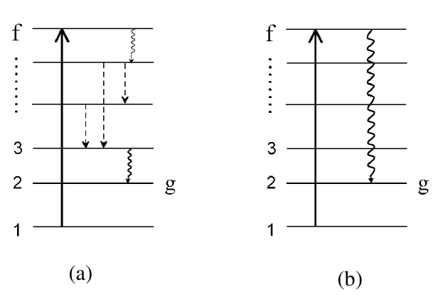
Figure 1: Schematic description of a nuclear excitation (solid line) followed by $\gamma$-decay (solid wavy line). (a) The dashed lines are transitions due to internal conversion (unobserved). The dashed wavy line is an unobserved $\gamma$-decay. (b) Direct emission of an observed gamma ray.

As for the non-relativistic case WB65 ; AW65 , the angular distributions of gamma rays following the excitation depend on the frame of reference used. In our notation, the z-axis corresponds to the beam axis, and the statistical tensors are given by (we use the notation of WB65 ; AW65 )

$$\alpha_{k\kappa}^{(0)}(f) =\frac{\left(2I_{f}+1\right)^{1/2}}{\left(2I_{1}+1\right)}\sum_{M_{f}=-(M_{f}^{{}^{\prime}}+\kappa),M_{f}^{{}^{\prime}}}\left(-1\right)^{I_{f}+M_{f}}\left(\begin{tabular}[c]{lll}$I$${}_{f}$&$I$${}_{f}$&$k$\\ $-M$${}_{f}$&$M$${}_{f}^{{}^{\prime}}$&$\kappa$\end{tabular}\right)$$ (90)

$$\times\sum_{M_{1}}a_{I_{f}M_{f}^{{}^{\prime}}}^{\ast}(M_{1})\;a_{I_{f}M_{f}}(M_{1})\;,$$ (91)

where $f$ is the state from which the gamma ray is emitted, and $1$ denotes the initial state of the nucleus, before the excitation. To calculate the angular distributions of the gamma rays one needs the statistical tensors for $k=0,2,4$ and $-k\leq\kappa\leq k$ (see WB65 ; AW65 ).

Instead of the diagram of figure 1(a), we will consider here the much simpler situation in which the $\gamma$-ray is emitted directly from the final excited state $f$ to a lower state $g$, which is observed experimentally (see figure 1(b)). The probability amplitude for this process is

$$a_{i\rightarrow f\rightarrow g}=\sum_{M_{f}}a_{i\rightarrow f}\;\left\langle I_{g}M_{g}\mathbf{k}\sigma\left|H_{\gamma}\right|I_{f}M_{f}\right\rangle,$$ (92)

where $\left\langle I_{g}M_{g}\mathbf{k}\sigma\left|H_{\gamma}\right|I_{f}M_{f}\right\rangle$ is the matrix element for the transition $f\rightarrow g$ due to the emission of a photon with momentum k and polarization $\sigma$. The operator $H_{\gamma}$ accounts for this transition. The angular dependence of the $\gamma$-rays is given explicitly by the spherical coordinates $\theta$ and $\phi$ of the vector k.

Since the angular emission probability will be normalized to unity, we can drop constant factors and write it as (an average over initial spins is included)

$$W\left(\theta\right)=\sum_{M_{i},\;M_{g},\sigma}\left|a_{i\rightarrow g}\right|^{2}=\sum_{M_{i},\;M_{g},\sigma}\left|\sum_{M_{f}}a_{i\rightarrow f}\;\left\langle I_{g}M_{g}\mathbf{k}\sigma\left|H_{\gamma}\right|I_{f}M_{f}\right\rangle\right|^{2}.$$ (93)

The transition operator $H_{\gamma}$ can be written as

$$H_{\gamma}=\sum_{lm}H_{\gamma}^{\left(lm\right)}=\sum_{lm}\hat{\mathcal{O}}_{lm}^{(nuc)}\otimes\hat{\mathcal{O}}_{lm}^{\left(\gamma\right)},$$ (94)

where the first operator in the sum acts between nuclear states, whereas the second operator acts between photon states of well defined angular momentum, $l,m$.

Expanding the photon state $\left|\mathbf{k}\sigma\right\rangle$ in a complete set $\left|lm\right\rangle$ of the photon angular momentum, and using the Wigner-Eckart theorem (angular momentum notation of ref. Ed60 ), one gets

$$\left\langle I_{g}M_{g}\mathbf{k}\sigma\left|H_{\gamma}\right|I_{f}M_{f}\right\rangle =\sum_{l,m}\left\langle\mathbf{k}\sigma|lm\right\rangle\left\langle I_{g}M_{g}\left|H_{\gamma}^{\left(lm\right)}\right|I_{f}M_{f}\right\rangle$$

$$=\left(-1\right)^{I_{f}-M_{f}}\sum_{l,m}\left(\begin{array}[c]{ccc}I_{f}&l&I_{g}\\ -M_{f}&m&M_{g}\end{array}\right)\left\langle\mathbf{k}\sigma|lm\right\rangle\left\langle I_{g}\left\|H_{\gamma}^{\left(l\right)}\right\|I_{f}\right\rangle.$$ (97)

One can rewrite $\left|\mathbf{k}\sigma\right\rangle$ in terms of $\left|\mathbf{z}\sigma\right\rangle$, i.e., in terms of a photon propagating in the z-direction. This is accomplished by rotating $\left|\mathbf{k}\sigma\right\rangle$ to the z-axis, using of the rotation matrix BS94 , $D_{mm^{\prime}}^{l}$, i.e.,

$$\left\langle\mathbf{k}\sigma|lm\right\rangle=\sum_{m^{\prime}}D_{mm^{\prime}}^{l}\left(\mathbf{z\longrightarrow k}\right)\left\langle\mathbf{z}\sigma|lm^{\prime}\right\rangle.$$ (98)

Expanding the photon field in terms of angular momentum eigenfunctions, one can show that FS65 ; EG88

$$\left\langle\mathbf{z}\sigma|lm\pi\right\rangle=\left\{\begin{array}[c]{c}\sqrt{\frac{2l+1}{2}}\delta_{\sigma m}\;\;\;\;\;\mathrm{for}\;\;\;\pi=E\\ \sqrt{\frac{2l+1}{2}}\sigma\delta_{\sigma m}\;\;\;\;\;\mathrm{for}\;\;\;\pi=M.\end{array}\right.$$ (99)

One has now to express the operator $\hat{\mathcal{O}}_{l^{\prime}m^{\prime}}^{\left(\gamma\right)}$ in eq. 94 in terms of the electric and magnetic multipole parts of the photon field. This problem is tedious but straightforward BR53 ). Inserting eqs. 98 and 99 in eq. 97, yields (neglecting constant factors)

$$\left\langle I_{g}M_{g}\mathbf{k}\sigma\left|H_{\gamma}\right|I_{f}M_{f}\right\rangle =\sum_{l,m}\left(-1\right)^{I_{g}-l+M_{f}}\sqrt{\left(2l+1\right)\left(2I_{f}+1\right)}\left(\begin{array}[c]{ccc}I_{g}&l&I_{f}\\ M_{f}&m&-M_{f}\end{array}\right)$$ (102)

$$\times D_{m\sigma}^{l}\left(\mathbf{z\longrightarrow k}\right)\left[\Delta_{El}+\sigma\Delta_{Ml}\right],$$ (103)

where $\Delta_{\pi l}$ is given by eq. 87.

Inserting eq. 103 into eq. 93 one gets a series of sums over the intermediate values of the angular momenta

$$W\left(\theta\right) =\sum_{\overset{M_{i},M_{g},\sigma,M_{f},}{M_{f}^{\prime},l,m,l^{\prime},m^{\prime}}}a_{i\longrightarrow f}a_{i\longrightarrow f^{\prime}}^{\ast}\sqrt{\left(2l+1\right)\left(2l^{\prime}+1\right)\left(2I_{f}+1\right)}\left(\begin{array}[c]{ccc}I_{g}&l&I_{f}\\ M_{g}&m&-M_{f}\end{array}\right)$$ (106)

$$\times\left(-1\right)^{M_{f}+M_{f}^{\prime}-l-l^{\prime}}\left(\begin{array}[c]{ccc}I_{g}&l^{\prime}&I_{f}\\ M_{g}&m^{\prime}&-M_{f}^{\prime}\end{array}\right)D_{m\sigma}^{l}\left[D_{m^{\prime}\sigma}^{l^{\prime}}\right]^{\ast}\Delta_{l}\Delta^{*}_{l^{\prime}}\;,$$ (109)

where $\Delta_{l}=\Delta_{El}+l\Delta_{Ml}$. The product $\Delta_{l}\Delta^{*}_{l^{\prime}}$ is always real since $(-1)^{s(l)}=\Pi$ (the parity).

Assuming that the particles are detected symmetrically around the z-axis one can integrate over $\phi_{particle}$, what is equivalent to integrating, or averaging, over $\phi_{\gamma}$. This yields the following integral

$$\int d\phi D_{m\sigma}^{l}\left[D_{m^{\prime}\sigma}^{l^{\prime}}\right]^{\ast}=$$

$$\delta_{mm^{\prime}}\left(-1\right)^{m-\sigma}\sum_{j}\frac{2j+1}{\sqrt{4\pi}}\left(\begin{array}[c]{ccc}l&j&l^{\prime}\\ m&0&-m\end{array}\right)\left(\begin{array}[c]{ccc}l&j&l^{\prime}\\ \sigma&0&-\sigma\end{array}\right)P_{j}\left(\cos\theta\right).$$ (114)

To simplify further eq. 109 we use (see ref. AW65 , p. 441, eq. II.A.61)

$$\sum_{M_{g}}\left(\begin{array}[c]{ccc}I_{g}&l&I_{f}\\ M_{g}&m&-M_{f}\end{array}\right)\left(\begin{array}[c]{ccc}I_{g}&l^{\prime}&I_{f}^{\prime}\\ M_{g}&m^{\prime}&-M_{f}^{\prime}\end{array}\right)$$ (119)

$$=\left(-1\right)^{2l^{\prime}-I_{g}}\sum_{k,\kappa}\left(-1\right)^{k+m-M_{f}^{\prime}}\left(2k+1\right)\left(\begin{array}[c]{ccc}l&l^{\prime}&k\\ m&-m^{\prime}&\kappa\end{array}\right)\left(\begin{array}[c]{ccc}I_{f}&I_{f}^{\prime}&k\\ M_{f}&-M_{f}^{\prime}&\kappa\end{array}\right)\left\{\begin{array}[c]{ccc}l&l^{\prime}&k\\ I_{f}^{\prime}&I_{f}&I_{g}\end{array}\right\}$$ (126)

and

$$\sum_{\sigma=\left(-1,1\right)}\left(\begin{array}[c]{ccc}l&j&l^{\prime}\\ \sigma&0&-\sigma\end{array}\right)\Delta_{\pi l}\Delta^{*}_{\pi l^{\prime}}=\left\{\begin{array}[c]{c}2\left(\begin{array}[c]{ccc}l&j&l^{\prime}\\ 1&0&-1\end{array}\right)\Delta_{\pi l}\Delta^{*}_{\pi l^{\prime}}\;,\;\;\;\;\;\mathrm{for}\;\;\;j=\mathrm{even}\\ 0\;,\;\;\;\;\;\;\;\;\;\mathrm{for}\;\;\;\;\;j=\mathrm{odd},\end{array}\right.$$

where use has been made of the parity selection rule

$$\Pi_{1}\Pi_{2}=\left\{\begin{array}[c]{c}\left(-1\right)^{l}\;,\;\;\;\mathrm{for}\;\;\;\mathrm{electric\;transitions}\\ \left(-1\right)^{l+1}\;,\;\;\;\mathrm{for}\;\;\;\mathrm{magnetic\;transitions\ .}\end{array}\right.$$

Eq. 109 becomes

$$W\left(\theta\right) =\sum_{\overset{M_{i},k,\kappa,M_{f},M_{f}^{\prime},}{l,l^{\prime},m,m^{\prime}}}\left(-1\right)^{2m^{\prime}+k+M_{f}}a_{i\longrightarrow f}a_{i\longrightarrow f^{\prime}}^{\ast}\sqrt{\left(2l+1\right)\left(2l^{\prime}+1\right)\left(2I_{f}+1\right)}$$

$$\times\left(2j+1\right)\left(2k+1\right)\left(\begin{array}[c]{ccc}I_{f}&I_{f}&k\\ M_{f}&-M_{f}^{\prime}&\kappa\end{array}\right)\left(\begin{array}[c]{ccc}I_{f}&l^{\prime}&k\\ M_{f}&-m^{\prime}&\kappa\end{array}\right)$$ (131)

$$\times\left(\begin{array}[c]{ccc}l&j&l^{\prime}\\ 1&0&-1\end{array}\right)\left(\begin{array}[c]{ccc}l&j&l^{\prime}\\ m&0&-m^{\prime}\end{array}\right)\left\{\begin{array}[c]{ccc}l&l^{\prime}&k\\ I_{f}^{\prime}&I_{f}&I_{g}\end{array}\right\}\Delta_{l}\Delta^{*}_{l^{\prime}}P_{j}\left(\cos\theta\right)\;.$$ (138)

Using

$$\sum_{m,m^{\prime}}\left(-1\right)^{2m^{\prime}}\left(\begin{array}[c]{ccc}l&j&l^{\prime}\\ m&0&-m^{\prime}\end{array}\right)\left(\begin{array}[c]{ccc}l&j&l^{\prime}\\ 1&0&-1\end{array}\right)=\left(-1\right)^{l+l^{\prime}+k}\frac{1}{2k+1}\delta_{kj}\delta_{\kappa 0},$$

one gets

$$W\left(\theta\right) =\sum_{\overset{k=\mathrm{even},M_{i},}{M_{f},l,l^{\prime}}}\left(-1\right)^{l+l^{\prime}+k}\sqrt{\left(2l+1\right)\left(2l^{\prime}+1\right)\left(2I_{f}+1\right)}\left(2k+1\right)\left|a_{i\longrightarrow f}\right|^{2}$$

$$\times\left(\begin{array}[c]{ccc}I_{f}&I_{f}&k\\ M_{f}&-M_{f}&0\end{array}\right)\left(\begin{array}[c]{ccc}l&j&l^{\prime}\\ 1&0&-1\end{array}\right)\left\{\begin{array}[c]{ccc}l&l^{\prime}&k\\ I_{f}^{\prime}&I_{f}&I_{g}\end{array}\right\}\Delta_{l}\Delta^{*}_{l^{\prime}}P_{j}\left(\cos\theta\right),$$

or in a more compact form

$$W\left(\theta\right)=\sum_{\overset{k=\mathrm{even},M_{i},M_{f},}{l,l^{\prime}}}\left(-1\right)^{M_{f}}\left|a_{i\longrightarrow f}\right|^{2}F_{k}\left(l,l^{\prime},I_{g},I_{f}\right)\left(\begin{array}[c]{ccc}I_{f}&I_{f}&k\\ M_{f}&-M_{f}&0\end{array}\right)\sqrt{2k+1}P_{k}\left(\cos\theta\right)\Delta_{l}\Delta^{*}_{l^{\prime}}\;,$$ (139)

where

$$F_{k}\left(l,l^{\prime},I_{g},I_{f}\right) =\left(-1\right)^{I_{f}-I_{g}-1}\sqrt{\left(2l+1\right)\left(2l^{\prime}+1\right)\left(2I_{f}+1\right)\left(2k+1\right)}$$

$$\times\left(\begin{array}[c]{ccc}l&l^{\prime}&k\\ 1&-1&0\end{array}\right)\left\{\begin{array}[c]{ccc}l&l^{\prime}&k\\ I_{f}&I_{f}&I_{g}\end{array}\right\}\ .$$ (144)

The angular distribution of $\gamma$-rays described above is in the reference frame of the excited nucleus. To obtain the distribution in the laboratory one has to perform the transformation

$$\theta_{L}=\arctan\left\{{\frac{\sin\theta}{\gamma\left[\cos\theta+\beta\right]}}\right\}\ ,$$ (145)

and

$$W(\theta_{L})=\gamma^{2}\left(1+\beta\cos\theta\right)^{2}W(\theta)\ ,$$ (146)

where $\gamma$ is given by eq. 35, and $\beta=\sqrt{1-1/\gamma^{2}}$. The photon energy in the laboratory is $E^{ph}_{L}=\gamma E^{ph}_{cm}\left(1+\beta\cos\theta\right)$.

XI.1 Computer program and user’s manual

All nuclear quantities, either known from experiments or calculated from a model, as well as the conditions realized in the experiment, are explicitly specified as input parameters. The program DWEIKO then computes the optical potentials (if required), differential cross section for elastic scattering, and Coulomb + nuclear excitation probabilities and cross sections, as well as the angular distribution of the $\gamma$-rays.

The units used in the program are fm (femtometer) for distances and MeV for energies. The output cross sections are given in millibarns.

XI.1.1 Input parameters

To avoid exceeding use of computer’s memory, the file DWEIKO.DIM contains the dimension of the arrays and sets in the maximum number of levels (NMAX), maximum total number of magnetic substates, (NSTMAX), maximum number of impact parameters (NBMAX), and maximum number of coordinates points used in the optical potentials and absorption factors, (NGRID). A good estimate is NSTMAX = $(2J_{max}+1)$NST, where $J_{max}$ is the maximum angular momentum of the input states.

Most integrals are performed by the 1/3-Simpson’s integration rule. It is required that NGRID be a even number, since an extra point (origin) is generated in the program.

The input file allows for comment lines. These should start with a ‘$\#$’ sign.

The file DWEIKO.IN contains all other input parameters. These are

1. AP, ZP, AT, ZT, which are the projectile and the target mass and charge numbers, respectively.

2. ECA, the bombarding energy per nucleon in MeV.

3. EX(j) and SPIN(j): the energy and spins of the individual states j.

4. MATE1(j,k), MATE2(j,k), MATE3 (j,k), MATM1(j,k), MATM2(j,k) the reduced matrix elements for E1, E2, E3 and M1, M2 excitations, $j\rightarrow k,$  (as defined in (48)), in $e$ fm (E1,M1), $e$ fm² (E2,M2), and $e$ fm⁴ (E3) units.

5. F(0,j), F(1,j), F(2,j), F(3,j), the fractions of sum rule of the deformation parameters for monopole, dipole, quadrupole, and octupole nuclear excitations, entering eq. (70).

   To simplify the input, the deformation parameters are calculated internally in DWEIKO using the sum rules 63-66, with $E_{x}$ replaced by the energy of the corresponding state, EX(j). The user needs to enter the fraction of those sum rules exhausted by the state j, i.e., the program uses $\delta_{\lambda}^{\prime}=f_{\lambda}\delta_{\lambda}$, with ($0\leq f_{\lambda}\leq 1$) entered by the user, and $\delta_{\lambda}$ given by eqs. 63-66.

The input cards in file DWEIKO.IN are organized as following:

1. AP, ZP, AT, ZT, ECA

   Charges and masses (AP,ZP,AT,ZT), bombarding energy per nucleon in MeV/nucleon.

2. IW, IOPM, IOELAS, IOINEL, IOGAM

   IW=0(1) for projectile (target) excitation.

   IOPM=1(0) for output (none) of optical model potentials.

   IOELAS=(0)[1]2 for (no output) [center of mass] laboratory elastic scattering cross section.

   IOINEL=(0)[1]2 for (no output) [center of mass] laboratory inelastic scattering cross section.

   IOGAM=(0)[1]2 for (no output) [output of statistical tensors] output of gamma-ray angular distributions.

   The statistical tensors are calculated for each impact parameter, so that one can use them in the computation of $dP_{\gamma N\rightarrow M}(b)/d\Omega_{\gamma}=P_{N}(b).dW_{\gamma N\rightarrow M}/d\Omega_{\gamma}$. If IW = 0, a transformation to the laboratory system is performed.

3. NB, ACCUR, BMIN, IOB

   NB = number of impact parameter points (NB $\leq$ NBMAX).

   ACCUR = accuracy required for the time integration of the CC-equations for each impact parameter. A reasonable value is ACCUR = 0.001, i.e., 0.1%.

   BMIN=minimum impact parameter (enter 0 for default. The program will integrate from $b=0$, with strong absorption included).

   IOB=1(0) prints (does not print) out impact parameter probabilities.

4. IOPW, IOPNUC

   IOPW is a switch for the optical potential model (OPM).

   IOPW=0 (no OMP, IOELAS=0), 1 (Woods-Saxon), 2 (read), 3 (t-$\rho\rho$ folding potential), 4 (M3Y folding potential).

   IOPNUC=0 (no nuclear), 1 (vibrational excitations).

   If the optical potential is provided (IOPW=2), it should be stored in ‘optw.in’ in rows of R x Real[U(R)] x Imag[U(R)]. The program makes an interpolation to obtain intermediate values.

   The first line in ‘optw.in’ is the number of rows (maximum=NGRID).

5. V0 [MeV], r0 [fm], d [fm], VI [MeV], r0$\_$I [fm], dI [fm]

   If IOPW=1, enter V0 [VI] = real [imaginary] part ($>$0) of Woods-Saxon potential, r0 [r0$\_$I] = radius parameter (R = r0 * (AP^1/3 + AT^1/3), d [dI] = diffuseness,

   If IOPW is not equal to 1, place a ‘$\#$’ sign at the beginning of this line, or delete it.

6. VS0 [MeV], r0$\_$S [fm], dS [fm], V$\_$surf [fm], a$\_$surf [fm]

   If IOPW=1 and AP, or AT, equal to one (proton), enter here spin-orbit part. If not, place a ’$\#$’ sign at the beginning of this line, or delete it.

   VS0 = depth parameter of the spin-orbit potential ($>$0), r0$\_$S = radius parameter, dS = diffuseness, V$\_$surf = depth parameter of the surface potential ($>$0), a$\_$surf = diffuseness,

7. Wrat

   If IOPW=4, enter Wrat = ratio of imaginary to real part of M3Y interaction.

   If IOPW is not equal to 4, place a ‘$\#$’ sign at the beginning of this line, or delete it.

8. THMAX, NTHETA

   If IOELAS=1,2 or IOINEL=1,2 enter here THMAX, maximum angle (in degrees and in the center of mass), and NTHETA ($\leq$ NGRID), the number of points in the scattering angle.

   If IOELAST or IOINEL are not 1, or 2, place a ‘$\#$’ sign at the beginning of this line, or delete it.

9. JINEL

   If IOINEL=1 enter the state (JINEL) for the inelastic angular distribution ($1<$ JINEL $\leq$ NST) .

   If IOINEL is not 1, or 2 place a ‘$\#$’ sign at the beginning of this line, or delete it.

10. NST

    NST ($\leq$ NMAX) is the number of nuclear levels.

11. I, EX(I), SPIN(I)

    Input of state labels (I), energy EX(I), and angular momentum SPIN(I). I ranges from 1 to NST and should be listed in increasing value of energies.

12. I, J, E1[e fm], E2[e fm²], E3[e fm³], M1[e fm], M2[e fm²]

    Reduced matrix elements for E1, E2, E3, M1 and M2 excitations: $<I_{j}||O(E/M;L)||I_{i}>$, j $\geq$ i , for the electromagnetic transitions. Matrices for reorientation effects, i$\rightarrow$i, can also be given.

    Add a row of zeros at the end of this list. If no electromagnetic excitation is wanted just enter a row of zeros.

13. J, F0, F1, F2, F3

    If IOPNUC=1 enter sum rule fraction of nuclear deformation parameters for monopole, dipole, quadrupole nuclear excitations (ALPHA0,DELTE1,DELTE2,DELTE3) for each excited state J.

    If IOPNUC=0 insert a comment card (‘$\#$’) in front of each entry row, or delete them.

14. IFF, IGG, THMIN, THMAX, NTHETA

    If IOGAM=2, enter IFF,IGG = initial and final states (IFF $>$ IGG) for the gamma transition.

    THMIN, THMAX = minimum and maximum values of gamma-ray angles (in degrees) in the laboratory frame.

    NTHETA = number of angle points ($\leq$ NGRID).

XI.1.2 Computer program

The program starts with a catalogue of the nuclear levels by doing a correspondence of integers to each magnetic substate. J = 1 corresponds to the lowest energy level, with the magnetic quantum number $M_{1}=-I_{1}$. J increases with $M_{1}$ and so on for the subsequent levels.

A mesh in impact parameter is done, reserving half of the impact parameter points, i.e., $NB/2$, to a finer mesh around the grazing impact parameter, defined as $b_{0}=1.2\left(A_{P}^{1/3}+A_{T}^{1/3}\right)\;$fm. The interval $b_{0}/3\;fm\leq b\leq 2b_{0}\;fm$ is covered by this mesh. A second mesh, with the other half of points, extends from $b=2b_{0}\;fm$ to $b=200\;fm.$ Except for the very low excitation energies ($E_{j}\ll 1$ MeV), combined with very large bombarding energies ($\gamma\gg 1$), this upper value of $b$ corresponds to very small excitation probabilities, and the calculation can be safely stopped. The reason for a finer mesh at small impact parameters is to get a good accuracy at the region where both nuclear, Coulomb, and absorption factors play equally important roles. At large impact parameters the probabilities fall off smoothly with $b$, justifying a wider integration step.

A mesh of NGRID points in polar coordinates is implemented to calculate the nuclear excitation potentials and absorption factors, according to the equations presented in sections 2.2 and 2.3. The first and second derivatives of the optical potentials are calculated by the routine DERIVATIVE. A 6-point formula is used for the purpose. The routines TWOFOLD computes the folding over the densities, as used in eq. (74). Routines RHOPP and RHONP generate the liquid drop densities, and the routine PHNUC computes the eikonal integral appearing in eq. (73).

Repeated factors for the nuclear and for the Coulomb potentials are calculated in the main program and stored in the main program with the arrays PSITOT and PSINUC. These arrays are carried over in a common block to the routine VINT which computes the function $Q_{N\lambda\mu}^{(kj)}(\xi_{kj},\tau)+Q_{C\pi\lambda\mu}(\xi_{kj},\tau)$, used in eq. (72).

The optical potentials are read in routine OMP$\_$READ, or calculated in routines OMP$\_$WS (Woods-Saxon), OMP$\_$DEN (t-$\rho\rho$) and OMP$\_$M3Y (M3Y). Routine TM3Y sets the M3Y interaction. DEFORM calculates the effective potentials in the Bohr-Mottelson model. SIGNNE and PHNNE return the nucleon-nucleon cross sections and the parameters of the nucleon-nucleon scattering amplitude 17. PHNUCF calculates the eikonal phase in the “t-$\rho\rho$” approximation with the help of the Fourier transform of the ground state densities, provided by FOURIER.

The time integrals are performed by means of an adaptive Runge-Kutta method. All routines used for this purpose have been taken from the Numerical Recipes Numrep . They are composed by the routines ODEINT, RKQS, RKCK, and RK4. The routine ODEINT varies the time step sizes to achieve the desired accuracy, controlled by the input parameter ACCUR. The right side of (72) is computed in the routine DCADT, used externally by the fourth-order Runge-Kutta routine RK4. RKCK is a driver to increase time steps in RK4, and RKQS is used in ODEINT for the variation of step size and accuracy control. The main program returns a warning if the summed errors for all magnetic substates is larger than 10 $\times$ ACCUR.

Elastic scattering is calculated within the routine ELAST for nucleus-nucleus, and ELASTP for proton-nucleus, collisions. Inelastic scattering is calculated within the routine INELAST, and $\gamma$-ray angular distributions are calculated in the routine GAMDIS.

The routine THREEJ computes Wigner-3J coefficients (and Clebsh-Gordan coefficients), RACAH the 6j-symbols, or Racah coefficients, YLM is used to compute the spherical harmonics, LEGENGC the Legendre polynomials, and BESSJ0 (BESSJ1) [BESSJN] the Bessel function $J_{0}$ ($J_{1}$) [$J_{n}$].

The routines SPLINE and SPLINT perform a spline interpolation of the excitation amplitudes, before they are used for integration by means of the routines QTRAP and QSIMP, from Numerical Recipes Numrep .

XII Test input and things to do

A test input is shown below. It corresponds to the excitation of giant resonance states in Pb by means of the reaction ¹⁷O (84 MeV/nucleon) + ²⁰⁸Pb. Assuming that an isolated state is excited, and that it exhausts fully the sum rules, one gets ($B(E\lambda)\equiv B(E\lambda,E_{x})$)

$$B(E1)={\frac{9}{4\pi}}\ {\frac{\hbar^{2}}{2m_{N}}}\ {\frac{NZ}{AE_{x}}}\ e^{2}\ ,$$ (147)

and, for ($\lambda>1$)

$$B(E\lambda)={\frac{3}{4\pi}}\ \lambda(2\lambda+1)\ {\frac{R^{2}}{E_{x}}}\ {\frac{\hbar^{2}}{2m_{N}}}\ e^{2}\times\left\{\begin{array}[c]{ll}Z^{2}/A,&\mbox{ for isoscalar excitations; }\\ NZ/A,&\mbox{for isovector excitations; }\end{array}\right.$$ (148)

From these values, the reduced matrix elements can be calculated from the definition in eq. 67.

Example 1 - The input list below calculates the excitation cross sections for the isovector giant dipole (IVGDR) and isoscalar giant quadrupole (ISGQR) resonances in Pb, for the above mentioned reaction. The user should first run this sample case and verify that the output numbers check those in ref. Ba88 . In particular, compare the results for elastic scattering with the upper figure 2 of ref. Ba88 . Also compare the inelastic excitation of the IVGDR with the upper figure 3 of ref. Ba88 . Following this it might be instructive to change the input of energies, spins, and excitation strengths for low lying states, giant resonances, etc.

$\#$   Input of program ‘DWEIKO’

$\#$   Ap   Zp   At   Zt   Einc[MeV/u]

17    8   208   82   84.   

$\#$   IW=0(1)   IOPM=0(1)   IOELAS=0(1)[2]   IOINEL=0(1)[2]   IOGAM=0(1)[2]

1   1   1   1   2

$\#$   NB   ACCUR   BMIN[fm]   IOB=1(0)

200   0.001   0.   0

$\#$   IOPW   IOPNUC

1   1

$\#$   V0 [MeV]   r0[fm]   d[fm]   VI [MeV]   r0$\_$I [fm]   dI [fm]

50.   1.067   0.8   58.   1.067   0.8

$\#$   VS0 [MeV]   r0$\_$S [fm]   dS [fm]   V_surf [fm]    d_surf

$\#$   15.   1.02   0.6   50.    0.8

$\#$   Wrat

$\#$    1.

$\#$   THMAX   NTHETA

6.   150

$\#$   JINEL

3

$\#$    NST

3

$\#$    I    Ex[MeV]   SPIN

1   0   0

2   10.9   2

3   13.5   1

$\#$   i -$>$ j   E1[e fm]   E2[e fm**2]   E3[e fm**3]   M1[e fm]   M2[e fm** 2]

1   2   0   76.8   0   0   0

1   3   9.3   0    0   0   0   

0   0   0    0   0     0   0

$\#$   j   F0   F1   F2   F3   (NOTE: fractions of sum rules for deformation parameters)

2   0   0   0.6   0

3   0   1.1   0   0

$\#$   IFF   IGG   THMIN   THMAX   NTHETA

2   1   20.   70.   150

Example 2 - Table III gives the results of an experiment on Coulomb excitation of S and Ar isotopes heiko . Choose the minimum impact parameter, BMIN, so that it reproduces the maximum scattering angle ($\theta_{\mathrm{max}}=4.1^{\circ}$) in the experiment (use the formula $b=a_{0}\cot({\theta/2})$ and read the last paragraph of section II). Using the $B(E2)$ values in the table reproduce the cross section values (careful with the units!).

Secondary beam	38S	40S	42S	44Ar	46Ar
$E_{\mathrm{lab}}$ [MeV/nucleon]	39.2	39.5	40.6	33.5	35.2
Energy of the first excited state [MeV]	1.286(19)	0.891(13	0.890(15)	1.144(17)	1.554(26)
$\sigma(E2;0_{g.s.}^{+}\rightarrow 2_{1}^{+};\ \theta_{\mathrm{lab}}\geq 4.1^{\circ})$ [mb]	59(7)	94(9)	128(19)	81(9)	53(10)
$B(E2;0_{g.s.}^{+}\rightarrow 2_{1}^{+})$ [$e^{2}$ fm4]	235(30)	334(36)	397(63)	345(41)	196(39)

Table III. Experimental results on Coulomb excitation of S and Ar projectiles impinging on a ¹⁹⁷Au target heiko .

Example 3 - Compare the results of this code with those from the ECIS code Ra72 ; Ra81 ; Ra87 . But notice that the ECIS code has relativistic corrections in kinematic variables only. The relativistic dynamics in the Coulomb and nuclear interaction are not accounted for. Thus, one should expect disagreements for high energy collisions ($E_{lab}\geq 100$ MeV/nucleon).

XIII Output

The output of DWEIKO are in the files

1. DWEIKO.OUT: Probabilities and cross sections;

2. DWEIKO$\_$OMP.OUT: Optical model potential;

3. DWEIKO$\_$ELAS.OUT: Elastic scattering cross section;

4. DWEIKO$\_$INEL.OUT: Inelastic scattering cross section;

5. DWEIKO$\_$STAT.OUT: Statistical tensors;

6. DWEIKO$\_$GAM.OUT: Angular distributions of gamma-rays.

XIV Acknowledgments

We would like to thank Ian Thompson for helping us to correct bugs in the program and for useful discussions. This material is based on work supported by the National Science Foundation under Grants No. PHY-0110253, PHY-9875122, PHY-007091 and PHY-0070818.

References

• (1) R.J. Glauber, “High-energy collisions theory”, in Lectures in Theoretical Physics, Interscience, NY, 1959, p. 315.
• (2) C.A. Bertulani, M.S. Hussein, and G. Münzenberg, Physics of Radioactive Beams (Nova Science Publishers, Huntington, NY, 2002).
• (3) G. Fäldt, Phys. Rev. D2, 846 (1970).
• (4) I. Thompson, Comp. Phys. Reports 7, 167 (1988).
• (5) P.D. Kunz and E. Rost, “The Distorted Wave Born Approximation”, published in Computational Nuclear Physics 2 - Nuclear Reactions, eds. K. Langanke, J.A. Maruhn and S.E. Koonin, Springer, NY, 1993.
• (6) H.M. Pilkuhn, Relativistic Particle Physics, Springer, NY, 1979.
• (7) C.E.Aguiar, A.N.F.Aleixo and C.A.Bertulani, Phys. Rev. C42, 2180 (1990); A.N.F.Aleixo and C.A.Bertulani, Nucl. Phys. A505, 448 (1989).
• (8) G.R. Satchler, “Direct Nuclear Reactions”, Oxford University Press, Oxford, 1983.
• (9) G. Bertsch, J. Borysowicz, H. McManus, and W.G. Love, Nucl. Phys. A284, 399 (1977).
• (10) A.M. Kobos, B.A. Brown, R. Lindsay, and G.R. Satchler, Nucl. Phys. A425, 205 (1984).
• (11) S. M. Lenzi, A. Vitturi, and F. Zardi, Phys. Rev. C38, 2086 (1988).
• (12) M.S. Hussein, R.A. Rego and C.A. Bertulani, Phys. Reports 201, 279 (1991).
• (13) H. Feshbach, “Theoretical Nuclear Physics: Nuclear Reactions”, ( Wiley-Interscience, Portland, 1993).
• (14) L. Ray, Phys. Rev. C20, 1857 (1979).
• (15) A. Vitturi and F. Zardi, Phys. Rev. C36, 1404 (1987).
• (16) N. Alamanos, Phys. Lett. B137, 37 (1984).
• (17) M. Buenerd et al., in Proc. Int. Conf. on Nuclear Physics, Florence, 1983, P. Blasi and R.A. Ricci, eds., (Tipografia Compositori, Bologna, 1983), p. 524.
• (18) A.K. Kerman, H. McManus and R.M. Thaler, Ann. Phys. (NY) 8, 551 (1959).
• (19) H. Goldstein, Classical Mechanics, Addison Wesley, NY, 1980.
• (20) C.A. Bertulani and G.Baur, Phys. Reports 163, 299 (1988).
• (21) T. Glasmacher, Ann. Rev. Nucl. Part. Sci. 48, 1 (1998).
• (22) A. Winther and K. Alder, Nucl. Phys. A319, 518 (1979)
• (23) K. Alder and A. Winther, “Coulomb Excitation”, Academic Press, New York, 1965.
• (24) J.M. Eisenberg and W. Greiner, “Excitation mechanisms of the nuclei”, North-Holland, Amsterdam, 1988.
• (25) C.A. Bertulani, L.F. Canto, M.S. Hussein and A.F.R. de Toledo Piza, Phys. Rev. C53 (1996) 334; C.A. Bertulani and V. Ponomarev, Phys. Rep. 321, 139 (1999).
• (26) C.A. Bertulani, Comp. Phys. Comm. 116, 345 (1999).
• (27) A.R. Edmonds, “Angular Momentum in Quantum Mechanics”, Princeton University Press, Princeton, New Jersey, 1960.
• (28) H. Esbensen and C.A. Bertulani, Phys. Rev. C65, 024605 (2002).
• (29) G.R. Satchler, Nucl. Phys. A472, 215 (1987).
• (30) W.D. Myers and W.J. Swiatecki, Ann. Phys. 55, 395 (1969); 84, 186 (1974).
• (31) C.A. Bertulani and A.M. Nathan, Nucl. Phys. A554, 158 (1993).
• (32) P.M. Morse and H. Feshbach, “Methods of Theoretical Physics”, McGraw Hill, NY, 1953.
• (33) A. Winther and J. De Boer, “A Computer Program for Multiple Coulomb Excitation”, Caltech, Technical report, November 18, 1965.
• (34) H. Frauenfelder and R.M. Steffen, “Alpha-, beta-, and gamma-ray spectroscopy”, Vol. 2, ed. K. Siegbahn.
• (35) D. Brink and G.R. Satchler, “Angular Momentum”, Oxford University Press, Oxford, 1953.
• (36) L.C. Biederharn and M.E. Rose, Rev. Modern Phys. 25, 729 (1953).
• (37) J. Barrete at al., Phys. Lett. B209, 182 (1988).
• (38) W.H. Press, B.P. Flannery, S.A. Teukolsky, and W.T. Vetterling, “Numerical Recipes”, Cambridge University Press, New York, 1996.
• (39) H. Scheit, T. Glasmacher, B. A. Brown, J. A. Brown, P. D. Cottle, P. G. Hansen, R. Harkewicz, M. Hellström, R. W. Ibbotson, J. K. Jewell, K. W. Kemper, D. J. Morrissey, M. Steiner, P. Thirolf, and M. Thoennessen, Phys. Rev. Lett. 77, 3967 (1996) .
• (40) J. Raynal, “Optical Model and Coupled-Channels Calculations in Nuclear Physics”, International Atomic Energy Agency report IAEA SMR-9/8, p. 281, Vienna(1972).
• (41) J. Raynal, Phys. Rev. C23, 2571 (1981).
• (42) J. Raynal, Phys. Lett. B196, 7 (1987).