Low Energy Expansion in the Three Body System to All Orders and the Triton Channel

Abstract

We extend and systematise the power counting for the three-body system, in the context of the “pion-less” Effective Field Theory approach, to all orders in the low-energy expansion. We show that a sub-leading part of the three-body force appears at the third order and delineate how the expansion proceeds at higher orders. After discussing the renormalisation issues in a simple bosonic model, we compute the phase shifts for neutron-deuteron scattering in the doublet $\mathrm{S}$ wave (triton) channel and compare our results with phase shift analysis and potential model calculations.

I Introduction

The disparity between the energy scales of typical QCD phenomena and the scale for nuclear binding makes nuclear systems an ideal playing ground for Effective Field Theory (EFT) methods. The first motivation behind the EFT program in nuclear physics is to obtain a description of nuclear phenomena firmly based on QCD. Recently, considerable effort has been put into the development of a phenomenologically successful EFT for nuclear physics [1, 2, 3, 4]. It soon became apparent that there is one feature which distinguishes the nuclear EFT from most of the many other applications of EFT methods: The low-energy expansion is non-perturbative in the sense that an infinite number of diagrams contribute at each order. This follows from the very existence of shallow real and virtual bound states whose binding energies are so small that they lie within the range of validity of the EFT even though they cannot be described by perturbing the free theory. In fact, there are at least in the two and three-nucleon sector states so loosely bound that their scales do not seem to be connected even to the soft QCD scales $m_{\pi}$ or $f_{\pi}$. Instead, they appear to require an additional “accidental” fine-tuning whose microscopic origin is not understood. However, this phenomenon offers the opportunity for a more radical use of EFT in the few nucleon case. In this approach, all particles but the nucleon themselves are considered high energy degrees of freedom and are consequently “integrated out”. The resulting EFT is considerably simpler than potential models or the “pionful” version of nuclear EFT (in which pions are kept as explicit degrees of freedom), but its range of validity is reduced to typical momenta below the pion mass. Albeit this might seem a severe restriction, there are many processes situated in this range which are both interesting in their own right and important for astrophysical applications. Also, we believe that an understanding of this simpler EFT is a necessary condition for understanding more general applications of EFT to nuclear physics and to other systems which exhibit shallow bound states.

The “pionless” EFT discussed here has its historical roots in the effective range expansion [5] and in the model-independent approach to three-body physics [6]. It considerably extends those approaches by making higher order calculations systematic, by including external electroweak currents, and by providing rigorous error estimates. A number of technical issues like gauge invariance and the inclusion of relativistic corrections are also much simpler in this approach. To gain perspective, it is useful at this point to briefly review what has been accomplished towards the “pionless” EFT program. In the two-nucleon sector, the modification of the power counting needed to deal with the fine tuning alluded to above and the resulting non-perturbative nature of the low-energy expansion is well understood. It has been phrased in elegant terms using dimensional regularisation which allows for analytical calculations. A large number of processes were analysed, some of them to very high order (see Refs. [1, 2, 3, 4] and references therein). Typically, most of the low-energy constants required are obtained from the plethora of available nucleon-nucleon scattering data. At some but usually high order, new two-body operators appear which describe effects due to “exchange currents”, “quark effects”, etc. They contribute typically in the range of a few percent to the final result. The coefficients of these operators are not constrained by nucleon-nucleon scattering data, but have to be fit to experiments in which the interaction of external currents with the two-nucleon system is probed. The low-energy expansion converges very nicely, the computations are not excessively complicated, and the only obstacle in obtaining arbitrary accuracy is the question whether there are enough data available to fix the low-energy constants.

In contradistinction, we are in the three-body sector still at a more primitive stage. For most channels of the three-nucleon system (without external currents), the approach used in the two-nucleon sector can be extended in a straightforward way. Analytical calculations, however, cannot be performed any more, as the basic Faddeev equation is no longer soluble in closed form. All these channels are repulsive, so that consequently no bound states exist, and the only observables are the nucleon-deuteron phase shifts which have been computed to third order [7, 8, 9, 10]. The only operators not determined by nucleon-nucleon data contributing to nucleon-deuteron scattering are three-body forces which are highly suppressed in these repulsive channels. In contradistinction, the ³He-³H channel exhibits the effect of the two-nucleon fine tuning much more dramatically. This leads to a very unusual situation. On a diagram-by-diagram basis, the graphs contributing at leading order (LO) to nucleon-deuteron scattering are finite. This seems to agree with the expectation, based on naïve dimensional analysis, that the three-body force, introduced to absorb any divergence, does not appear at leading order. However, it turns out that the ultraviolent behaviour of the equation describing the three-body system is very different from the behaviour of its perturbative expansion. In particular, a non-derivative three-body force is required to absorb cutoff dependences already at leading order. This immediately voids the use of the effective range expansion. The precise value of the three-body force is not determined by nucleon-nucleon data and has to be determined by some additional three-nucleon datum. These unusual properties of the Faddeev equation and the existence of a new free parameter in the three-body sector was recognised early on [11], and the renormalisation theory interpretation was given in [12]. These complications hindered the extension of a consistent and economical power counting to the three-body sector, and currently only leading and next-to-leading order (NLO) calculations of the doublet $\mathrm{S}$-wave neutron deuteron phase shift and of the corresponding triton binding energy are available [13, 14]. To attain the precision necessary to be of phenomenological interest, one has to go at least one order beyond that.

This paper is devoted to re-formulating the renormalisation issues in the ³He-³H sector in order to extend the power counting to all orders. In the following section, we do so first in a bosonic model to avoid unrelated complications coming from the spin-isospin structure. In Sect. III, we consider the three-nucleon system, and compute then the neutron-deuteron phase shift in this channel at next-to-next-to-next leading order (NNLO) in Sect. IV. There, we also compare the results with the available phase shift analysis [15], and with potential model calculations [16]. This also allows us to discuss the convergence of the low-energy expansion in order to obtain a credible error estimate. We close by conclusions, outlook and an appendix.

II Bosonic interlude: Power counting to all orders

Let us first consider the renormalisation of higher order corrections in the simpler setting of the model of three spinless bosons of mass $M$ whose two body system exhibits a shallow real bound state. This avoids the technical complications with spin and isospin degrees of freedom. The Lagrangean is thus

$$\begin{split}{\mathscr{L}}=\psi^{\dagger}\left(\mathrm{i}\partial_{0}+\frac{\nabla^{2}}{2M}\right)\psi&+\frac{C_{0}}{4}|\psi|^{4}+\frac{C_{2}}{4}\left((\psi^{\dagger}(\overrightarrow{\nabla}-\overleftarrow{\nabla})^{2}\psi^{\dagger})\psi^{2}+\text{H.c.}\right)\hfill\\ &+\hfill\frac{D_{0}}{36}|\psi|^{6}+\frac{D_{2}}{36}\left((\psi^{\dagger}(\overrightarrow{\nabla}-\overleftarrow{\nabla})^{2}\psi^{\dagger})\psi^{\dagger}\psi^{3}+\text{H.c.}\right)+\dots\;\;,\end{split}$$ (1)

where the terms not explictly shown are further suppressed. A more convenient form of writing the same theory is obtained by introducing two dummy fields $d$ and $t$ with the quantum numbers of two and three particles (referred to in this section as the “deuteron” and “triton”)

$$\begin{split}{\mathscr{L}}=\psi^{\dagger}\left(\mathrm{i}\partial_{0}+\frac{\nabla^{2}}{2M}\right)\psi&+d^{\dagger}\left(-\mathrm{i}\partial_{0}-\frac{\nabla^{2}}{4M}+\Delta\right)d+t^{\dagger}\left(\mathrm{i}\partial_{0}+\frac{\nabla^{2}}{6M}+\frac{\gamma^{2}}{M}+\Omega\right)t\\ &-\frac{g}{\sqrt{2}}\left(d^{\dagger}\psi^{2}+\text{H.c.}\right)-\omega\left(t^{\dagger}d\psi+\text{H.c.}\right)+\dots\;\;.\end{split}$$ (2)

The equivalence between the two Lagrangeans (1) and (2) is established by performing the Gaußian integral over the auxiliary fields $d$ and $t$ and disregarding terms with more fields and/or derivatives, that are suppressed further [9]. However, there is a subtlety. In order to eliminate time derivatives and express the result of this integration in a manifestly boost invariant way as in (1), one has to perform a field redefinition

$$\psi\rightarrow\psi+\frac{g^{2}}{2\Delta^{2}}|\psi|^{2}\psi+\left(\frac{7g^{4}}{8\Delta^{4}}-\frac{3g^{2}\omega^{2}}{4\Delta^{2}\Omega^{2}}\right)|\psi|^{4}\psi\;\;.$$ (3)

The relation between the constants in the two Lagrangeans is then given by

$$\begin{split}C_{0}&=-\frac{2g^{2}}{\Delta}\;\;,\\ C_{2}&=\frac{1}{4M}\frac{g^{2}}{\Delta^{2}}\;\;,\\ D_{0}&=-\frac{18g^{2}\omega^{2}}{\Omega\Delta^{2}}\;\;,\\ D_{2}&=\frac{21g^{2}}{4M\Delta^{4}}-\frac{9g^{2}\omega^{2}}{2M\Omega^{2}\Delta^{2}}\;\;.\end{split}$$ (4)

We can identify three scales in the problem: $Q$ is a typical external momentum, $R$ is the short distance scale in position space beyond which the EFT breaks down, and $\gamma=\sqrt{MB_{2}}$ the anomalously small binding momentum of the shallow two boson bound state of binding energy $B_{2}$. This scale is, up to effective range corrections, equal to the inverse scattering length in the two-body channel. We thus perform an expansion in powers of two small dimensionless numbers, $QR\ll 1$ and $\gamma R\ll 1$, while keeping terms with arbitrary powers of $Q/\gamma\sim 1$. The corresponding power counting has been extensively discussed elsewhere and will not be repeated here, see e.g. [1, 2, 3] and references therein. Its details depend on the particular regularisation and renormalisation scheme used. In this work, we use a sharp momentum cutoff to regulate divergent integrals. The result of these considerations can be summed by stating which diagrams contribute at each order in the low-energy expansion.

The bare deuteron propagator is given by the constant term $\mathrm{i}/\Delta$. At leading order (LO), the $d$ field propagator is given by the sum of all graphs made up from the interaction proportional to $g$ in (2) with an arbitrary number of loops, see Fig. 1.

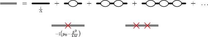
Figure 1: Top: Re-summation of the bare deuteron propagator (thick solid line) into the dressed deuteron propagator (double line) at LO by dressing with two-nucleon bubbles. Bottom: The NLO and NNLO corrections to the deuteron propagator. The cross denotes an insertion of the deuteron kinetic energy operator.

At next-to-leading order (NLO), one includes one perturbative insertion of the deuteron kinetic term. At next-to-next-to-leading order (NNLO), two insertions of the kinetic energy enter. At higher orders, terms with more derivatives not explicitly shown in (2) appear. We thus arrive at the deuteron propagator in the low-energy expansion

$$\bar{\mathcal{D}}(p_{0},p) = \bar{\mathcal{D}}^{(0)}(p_{0},p)+\bar{\mathcal{D}}^{(1)}(p_{0},p)+\bar{\mathcal{D}}^{(2)}(p_{0},p)+\mathcal{O}(p^{3}R^{3})$$

$$= \frac{4\pi}{Mg^{2}}\left[\frac{1}{-\gamma+\sqrt{-Mp_{0}+\frac{p^{2}}{4}-\mathrm{i}\epsilon}}-\frac{\rho}{2}\frac{\gamma^{2}+Mp_{0}-\frac{p^{2}}{4}}{\left(-\gamma+\sqrt{-Mp_{0}+\frac{p^{2}}{4}-\mathrm{i}\epsilon}\right)^{2}}\right.$$

$$\left.+\left(\frac{\rho}{2}\right)^{2}\frac{(\gamma^{2}+Mp_{0}-\frac{p^{2}}{4})^{2}}{\left(-\gamma+\sqrt{-Mp_{0}+\frac{p^{2}}{4}-\mathrm{i}\epsilon}\right)^{3}}\right]+{\mathcal{O}}(p^{3}R^{3})$$

$$\equiv \frac{4\pi}{Mg^{2}}\mathcal{D}(p_{0},p)\;\;,$$

where $\rho$ is the effective range, defined by performing the effective range expansion around the bound state. The effective range is assumed to be of natural size, $\rho\sim R$. We also defined the rescaled propagator $\mathcal{D}(p_{0},p)$ for future convenience and quote the two particle propagator when the effective range is summed to all orders, but the other corrections in the effective range expansion are left out:

$$\mathcal{D}(p_{0},p)\to\frac{1}{-\gamma+\sqrt{-Mp_{0}+\frac{p^{2}}{4}-\mathrm{i}\epsilon}+\frac{\rho}{2}\left(\gamma^{2}+Mp_{0}-\frac{p^{2}}{4}\right)}\;\;.$$ (6)

The two particle scattering amplitude is obtained from the $d$ field propagator by multiplying it by $g^{2}$. After that, we recognise the familiar form of the scattering amplitude in the effective range expansion, which had allowed us to determine the low-energy constants $C_{0},C_{2}$ in terms of $\gamma$ and $\rho$ in (II/6).

Similarly, the leading order three-particle amplitude includes all diagrams build up of the leading two-body interactions, i.e. the ones proportional to $C_{0}$ in (1) or $g$ and $\Delta$ in (2). The NLO amplitude includes the graphs with one insertion of the deuteron kinetic energy, the NNLO amplitude includes those with two deuteron kinetic energy insertions, and at higher orders new interactions not explicitly shown in (1/2) appear. But that is not all. There also appear graphs containing the three-body interactions proportional to $D_{0},D_{2}$ in (1) or $\Omega$ and the triton kinetic energy in (2). It has been established that the leading three body force, i.e. the one proportional to $D_{0}$ in (1) or $\Omega$ in (2) appears at LO and NLO [12, 13, 14]. We will re-derive this fact in a slightly modified way which permits us also to find the proper generalisation to all orders in the expansion.

Our argument proceeds as follows. We include a specific three-body force term at a given order $n$ of the expansion if and only if that term is needed to cancel cutoff dependences in the observables which are stronger than cutoff dependence from the suppressed terms of order $(QR)^{n+1}$. The rationale we follow is thus simply a consequence of the fact that physical observables cannot depend on the arbitrary value of the cutoff and, from the point of view of the EFT, cutoff dependences coming from loops and from the values of the low-energy constants cancel order by order in the expansion.

Before we implement this idea, let us make a few comments about the economy of computing diagrams at high orders. There is an infinite number of diagrams contributing at leading order, as shown in Fig. 2.

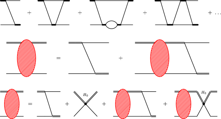
Figure 2: Re-summation of the naïve LO three-body equation, without three-body interactions (top), into the corresponding Faddeev integral equation (mid) for the Boson case. Bottom: The same including three-body interactions with strength $H_{0}(\Lambda)$, denoted by the dot. Remaining notation as in Fig. 1.

We sum them up by solving the Faddeev integral equation for point-like interactions. In the case where only two-body interactions are present, this equation was first derived in [17]. This re-summation is necessary since – according to the power counting – all these diagrams contribute equally to the final amplitude. The NLO contribution can then be obtained by perturbing around the LO solution with the deuteron kinetic energy operator, as shown diagrammatically in Fig. 3.

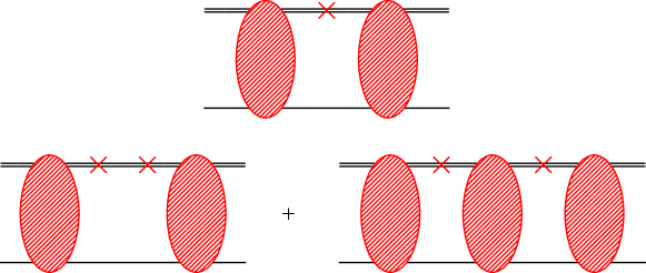
Figure 3: The graphs to be computed when inserting the higher order corrections to the deuteron propagator perturbatively. Top: NLO. Bottom: NNLO. The bottom right diagram makes the knowledge of the full off-shell LO amplitude mandatory. Notation as in Fig. 1.

This approach was taken before and is easily implemented [14]. However, it suffers a drawback at higher orders because one must then insert the kinetic energy operator two or more times. This is very cumbersome to do numerically, particularly because of the need to compute the full off-shell LO amplitude before inserting the deuteron kinetic energy terms, see Fig. 3. A more practical method would be to re-sum all range corrections into the deuteron propagator and solve a modified integral equation. This approach has its own drawbacks, including the existence of spurious bound states in the re-summed deuteron propagator, and was shown to fail miserably for the phase shifts [18].

We choose a middle ground: First, expand the kernel of the integral equation perturbatively, and then iterate it by inserting it into the integral equation. That means, we perform a partial re-summation of the range effects: We use the deuteron propagator in (II) in the integral equation, which is then solved numerically. Figure 4 shows a graphical representation of the NLO version. This procedures includes some graphs of higher order, for instance, the NLO calculation includes diagrams like the bottom right one in Fig. 3, but not diagrams like the bottom left one in the same Figure. The partial re-summation arbitrarily includes higher order graphs and consequently does not improve the precision of the calculation. But the additional diagrams are small in a well-behaved expansion, so the precision is not compromised, either. On the other hand, this prescription is much easier to handle numerically than the two other methods. In a nutshell, the only necessary re-summation is the one present at LO. The partial re-summation of range effects is made only for convenience.

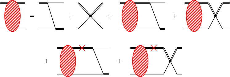
Figure 4: The integral equation for the boson case when the kernel is expanded to NLO. Notation as in Figs. 1 and 2.

The integral equation describing particle-deuteron scattering one obtains by including the re-summation discussed above is hence a minor modification of the one derived in [17, 12]. Its NLO version is graphically represented in Fig. 4. The integral equation for the half off-shell amplitude up to and including NNLO reads:

$$t_{\Lambda}(p,k)=\mathcal{K}(p,k)+\mathcal{H}(p,\Lambda)+\frac{2}{\pi}\int\limits_{0}^{\Lambda}\mathrm{d}q\;q^{2}\mathcal{D}(E-\frac{q^{2}}{2M},q)\left[\mathcal{K}(p,q)+\mathcal{H}(E,\Lambda)\right]t_{\Lambda}(q,k)\;\;,$$ (7)

where

$$\mathcal{H}(E,\Lambda) = \mathcal{H}_{0}(\Lambda)+\mathcal{H}_{2}(E,\Lambda)\;\;,$$ (8)

$$\mathcal{H}_{0}(\Lambda) = \frac{2H_{0}(\Lambda)}{\Lambda^{2}}=-\frac{\omega^{2}}{4Mg^{2}\Omega}\;\;,$$ (9)

$$\mathcal{H}_{2}(E,\Lambda) = \frac{2H_{2}(\Lambda)}{\Lambda^{4}}\;(ME+\gamma^{2})=\frac{\omega^{2}}{4Mg^{2}\Omega^{2}}\;(ME+\gamma^{2})\;\;,$$ (10)

$$\mathcal{K}(p,q) = \frac{1}{pq}\ln\left(\frac{p^{2}+pq+q^{2}-ME}{p^{2}-pq+q^{2}-ME}\right)\;\;,$$ (11)

and $E=3k^{2}/(4M)-\gamma^{2}/M$ is the total centre-of-mass energy. The on-shell scattering amplitude $T(k)$ is given by $Zt_{\Lambda}(k,k)$ , where the deuteron wave function renormalisation factor is given by

$$Z=\frac{8\pi\gamma}{M}\left(1+\gamma\rho+(\gamma\rho)^{2}+\dots\right)\;\;.$$ (12)

and is related to the phase shift $\delta$ in this channel by the usual formula

$$T(k)=Zt_{\Lambda}(k,k)=\frac{3\pi}{M}\frac{1}{k\cot\delta-\mathrm{i}k}\;\;.$$ (13)

As (7) contains the cutoff $\Lambda$, the solution $t_{\Lambda}(q)$ for arbitrary $H_{0},H_{2}$ depends in general on the cutoff, too. Since the low-energy amplitude can not depend on the cutoff, any explicit dependence on the cutoff has to be cancelled by the cutoff dependence implicit in $H_{0},H_{2}$, etc. We determine the cutoff dependence of the three-body forces by imposing this condition order by order in $1/\Lambda$. In this process, we also determine which three-body force appears at every order of the expansion.

Let us first consider the effect of changing the cutoff from $\Lambda$ to $\Lambda^{\prime}\sim\Lambda$. The equation satisfied by the amplitude $t_{\Lambda^{\prime}}$ analogous to (7) can be written as follows:

$$\int\limits_{0}^{\Lambda}\!\mathrm{d}q\;\underbrace{\Big{(}\delta(p-q)}_{\sim 1/Q^{2}}-\frac{2}{\pi}\underbrace{q^{2}\mathcal{D}(E-\frac{q^{2}}{2M},q)\mathcal{K}(p,q)\Big{)}}_{\sim 1/Q^{2}}t_{\Lambda^{\prime}}(q)=\underbrace{\mathcal{K}(p,k)}_{\sim 1/Q^{2}}+\underbrace{\mathcal{H}(E,\Lambda)}_{\sim 1/\Lambda^{2}}$$

$$+\frac{2}{\pi}\underbrace{\int\limits_{0}^{\Lambda}\mathrm{d}q\;q^{2}{\mathcal{D}}(q)\mathcal{H}(E,\Lambda)t_{\Lambda^{\prime}}(q)}_{\sim 1/(Q\Lambda)}$$

$$+\frac{2}{\pi}\underbrace{\int\limits_{0}^{\Lambda}\mathrm{d}q\;q^{2}\mathcal{D}(E-\frac{q^{2}}{2M},q)(\mathcal{H}(E,\Lambda^{\prime})-\mathcal{H}(E,\Lambda))t_{\Lambda^{\prime}}(q)}_{\sim 1/(Q\Lambda)}$$

$$+\underbrace{\mathcal{H}(E,\Lambda^{\prime})}_{\sim 1/\Lambda^{2}}-\underbrace{\mathcal{H}(E,\Lambda)}_{\sim 1/\Lambda^{2}}$$

$$+\frac{2}{\pi}\int\limits_{\Lambda}^{\Lambda^{\prime}}\mathrm{d}q\;q^{2}\mathcal{D}(E-\frac{q^{2}}{2M},q)\underbrace{\Big{(}\mathcal{K}(p,q)}_{\sim 1/(Q\Lambda)}+\underbrace{\mathcal{H}(E,\Lambda^{\prime})\Big{)}}_{\sim 1/(Q\Lambda)}t_{\Lambda^{\prime}}(q)$$ (14)

The point of this rewriting is to show explicitly as in the last three lines the difference between the equations satisfied by $t_{\Lambda}(p)$ and $t_{\Lambda^{\prime}}(p)$. Now we take the cutoffs $\Lambda$ and $\Lambda^{\prime}$ to be below the short distance scale $Q\ll\Lambda\ll 1/r\sim 1/R$, but higher than the infrared scales $Q\sim\gamma\sim k\sim p$. The asymptotic behaviour of $t(q)$ is known to be of the form $t(p\gg Q)\sim\sin(s_{0}\ln p/\bar{\Lambda})/(Qp)$ [19] (see Appendix), so $t(p\sim Q)\sim 1/Q^{2}$ and $t(p\sim\Lambda)\sim 1/(Q\Lambda)$. As one knows the asymptotic behaviour of $t_{\Lambda}(p)$ and assumes $H_{0}\sim H_{2}\sim 1$, one can estimate the size of each term in (II) as shown in under-braces. Here, loop momenta $q$ count as $Q$ in ultraviolet finite integrals but count as $\Lambda$ in divergent integrals, since the integrals are dominated by momenta of the order $Q$ and $\Lambda$, respectively.

The estimate suggests that the terms on the right hand side describing the contribution from loop momenta between $\Lambda$ and $\Lambda^{\prime}$ as well as the contribution from the three-body forces are small compared to the leading ones on the left hand side, the former being suppressed by at least one power of $Q/\Lambda$. Therefore, one naïvely expects them to be negligible at leading order. If one indeed discards them, the resulting equation for $t_{\Lambda^{\prime}}(p)$ becomes identical to (7) and one has to conclude that $t_{\Lambda^{\prime}}(p)\simeq t_{\Lambda}(p)+\mathcal{O}(Q/\Lambda)$.

The argument above is, however, incorrect. This is due to the fact that left hand side of (II) is singular in the limit $\Lambda\rightarrow\infty$. More precisely, in this limit, there is a zero eigenvalue for the operator on the left hand side of (II) acting on $t_{\Lambda}^{\prime}(p)$:

$$\int\limits_{0}^{\infty}\!\mathrm{d}q\;\left(\delta(p-q)-\frac{2}{\pi}q^{2}\mathcal{D}(E-\frac{q^{2}}{2M},q)\mathcal{K}(p,q)\right)a(p)=0\;\;.$$ (15)

We refer the reader to Ref. [11] which proves this statement rigorously and also makes it clear that the spectrum of the operator in (15) is continuous. One important point to notice is that the existence of the zero mode is an ultraviolet phenomenon, independent of the infrared scales like $E$ or $\gamma$. In the simpler case $\gamma=0$, the eigenfunction corresponding to an eigenvalue $\lambda$ can be expressed analytically at LO as

$$a_{\lambda}(p)=\sin\left(-\mathrm{i}s\ln\left(\sqrt{\frac{-3p^{2}}{4ME}}+\sqrt{1-\frac{3p^{2}}{4ME}}\right)\right)$$ (16)

with eigenvalue

$$\lambda=1-\frac{8}{\sqrt{3}s}\frac{\sin(\pi s/6)}{\cos(\pi s/2)}$$ (17)

and $-1<\mathrm{Re}(s)<1$ The zero mode $a_{0}(p)$ corresponds to $s(\lambda=0)=\mathrm{i}s_{0}=\mathrm{i}\;1.00624\dots$. The existence of the zero mode shows that for $\Lambda\rightarrow\infty$, the operator on the left hand side of (7) has no inverse. Therefore, the solution to the integral equation is not unique since one can always add $a_{0}(p)$ to a given solution and obtain another valid solution.

For finite $\Lambda$, general theorems guarantee that the spectrum of the operator is discrete [20]. Eq. (7) then defines the amplitude uniquely. However, as $\Lambda$ is increased the eigenvalues get closer to each other and, for a generic value of the cutoff, the eigenvalue closest to zero is of the order $\mathcal{O}(Q/\Lambda)$. Since the operator in the left hand side of (7) is nearly singular, terms of order $\mathcal{O}(Q/\Lambda)$ on the right hand side of (II) can have an effect on $t_{\Lambda}(p)$ of order $\mathcal{O}(1)$. This “hypersensitivity” to cutoff dependences is at the heart of the apparently paradoxical fact that the solution of (7) with $\mathcal{H}=0$ is cutoff dependent, even though the contribution of the high momentum modes are suppressed by $1/\Lambda$ (that is, are ultraviolet finite). In general, for the amplitude to be cutoff independent up to terms of order $\mathcal{O}((Q/\Lambda)^{n})$ , the right hand side of (II) has to be cutoff independent up to terms of order $\mathcal{O}((Q/\Lambda)^{n+1})$ , i.e. one order higher than in the standard cases. Notice that the unexpected dependence of the low-energy amplitude on high momenta is due to two factors: the harder asymptotic behaviour of $t(p)\sim 1/p$ compared to the perturbation theory expectation $t(p)\sim 1/p^{2}$, and the fact that the leading terms in (II) form a nearly singular equation that amplifies any remaining term by one power of $\Lambda/Q$.

We now determine the three-body forces by demanding order by order in $Q/\Lambda$

$${\mathcal{H}}(E,\Lambda)+\frac{2}{\pi}\int\limits^{\Lambda}\mathrm{d}q\;q^{2}\mathcal{D}(E-\frac{q^{2}}{2M},q)\left[{\mathcal{K}}(q,p)+{\mathcal{H}}(E,\Lambda)\right]t_{\Lambda}(q)=\mathrm{const.}\;\;,$$ (18)

i.e. the amplitude must be cutoff independent. This (possibly energy dependent) constant can without loss of generality be set to zero by absorbing it into a re-defined three body force

$$\mathcal{H}(E,\Lambda)\to\mathcal{H}(E,\Lambda)-\frac{\mathrm{const.}}{1+\displaystyle\frac{2}{\pi}\int\limits^{\Lambda}\mathrm{d}q\;q^{2}\mathcal{D}(E-\frac{q^{2}}{2M},q)\;t_{\Lambda}(q)}\;\;.$$ (19)

Imposing (18) with $\mathrm{const.}=0$ order by order in the low energy expansion, we can determine which three-body forces are required at any given order, and how they depend on the cutoff. As we are interested only in the UV behaviour, i.e. in the asymptotics, and no IR divergences occur, we can safely neglect the IR limit of the integral.

At leading order, $\gamma\ll\Lambda$, and we can approximate

$$\begin{split}\mathcal{D}(E-\frac{q^{2}}{2M},q)&\simeq\sqrt{\frac{4}{3}}\frac{1}{q}+\dots\;\;,\\ {\mathcal{K}}(q,p)&\simeq\frac{2}{q^{2}}+\dots\\ {\mathcal{H}}(E,\Lambda)&\simeq\frac{2H_{0}(\Lambda)}{\Lambda^{2}}+\dots\\ t(q)&\simeq A(k/\Lambda,\gamma/\Lambda)\frac{\sin[s_{0}\ln(q/\bar{\Lambda})]}{q}+\dots\;\;.\end{split}$$ (20)

where a normalisation factor $A$ was included into the asymptotic form of $t(q)$. The essential observation is that the terms of order $\mathcal{O}(Q/\Lambda)$ are independent of $E$ (or $k$) and hence can be made to vanish by adjusting only $H_{0}$ and not $H_{2}$ or any of the higher derivative three-body forces. In fact, using the substitutions of (20) in (18) and neglecting higher order corrections for naturally-sized $H_{0}$, we find

$$H(\Lambda)=\frac{\sin[s_{0}\ln\frac{\Lambda}{\bar{\Lambda}}+\arctan s_{0}]}{\sin[s_{0}\ln\frac{\Lambda}{\bar{\Lambda}}-\arctan s_{0}]}$$ (21)

as obtained previously [12].

At NLO, we impose (18) to order $\mathcal{O}(1/\Lambda^{2})$. Thus, we expand one order higher than (20)

$$\begin{split}\mathcal{D}(E-\frac{q^{2}}{2M},q)&\simeq\sqrt{\frac{4}{3}}\frac{1}{q}+\frac{4}{3}\frac{\gamma}{q^{2}}+\frac{r}{2}\dots\ \\ {\mathcal{K}}(q,p)&\simeq\frac{2}{q^{2}}+\dots\\ {\mathcal{H}}(E,\Lambda)&\simeq\frac{2H_{0}(\Lambda)}{\Lambda^{2}}+\dots\;\;.\end{split}$$ (22)

The sub-leading asymptotics at NLO depends on whether $\Lambda\ll 1/r$ or $\Lambda\gg 1/r$. In the first case, there is only a perturbative change from the LO asymptotics, and we can find it analytically (see Appendix)

$$\begin{split}t(q)\simeq A(k/\Lambda)\Big{[}\frac{\sin[s_{0}\ln(q/\bar{\Lambda})]}{q}&+|B_{1}|\;r\sin[s_{0}\ln(q/\bar{\Lambda})+\arg(B_{1})]\\ &+|B_{-1}|\;8\gamma\frac{\sin[s_{0}\ln(q/\bar{\Lambda})+\arg(B_{-1})]}{q^{2}}+\dots\Big{]}\;\;.\end{split}$$ (23)

Again we see that, to this order, no terms dependent on $E$ or $k$ are present. Only the $H_{0}(\Lambda)$ term is necessary for renormalisation. Plugging (22/23) back in (18) and keeping only the terms of order $1/\Lambda^{2}$, one can derive the sub-leading correction to (21), but the expression is long and of no immediate use.

A new three-body force enters at NNLO. We require now that the terms of order $(Q/\Lambda)^{3}$ on the right hand side of (II) should vanish, which guarantees that the amplitude is cutoff independent up to terms of order $(Q/\Lambda)^{2}$. At this order though, there are terms proportional to $ME$ arising from expanding the kernel in powers of $q/\Lambda$ and $\sqrt{ME}/\Lambda$. Indeed, such corrections appear only at even orders. Only a three-body force term which also contains a dependence on the external momenta $k^{2}$ and $ME$ (both equivalent on-shell) can absorb them. That means that $H_{2}$ appears at NNLO. In addition, there is a large number of momentum independent terms that renormalise $H_{0}$ and provide the NNLO corrections to (21). The same pattern repeats at higher orders. Every two orders, a new three-body force term appears with two extra derivatives, guaranteeing that the new three-body forces are analytic in $ME\propto k^{2}$ on shell.

If we choose $\Lambda\gtrsim 1/r$, the argument is changed only by the change in the asymptotic form of $t(p)$. This affects the explicit forms for the running of $H_{0},H_{2}$, but not the fact that they are necessary and sufficient to perform the renormalisation.

III Three nucleons in the triton channel

It is not difficult to include the spin and isospin degrees of freedom and generalise the discussion in the previous section to the case of the three-nucleon system. As discussed elsewhere, the ${}^{2}\mathrm{S}_{\frac{1}{2}}$ channel – to which ³He and ³H belong – is qualitatively different from the other three-nucleon channels. This difference can be traced back to the effect of the exclusion principle and the angular momentum repulsion barrier. In all the other channels, it is either the Pauli principle or an angular momentum barrier (or both) which forbids the three particles to occupy the same point in space. As a consequence, the kernel describing the interaction among the three nucleons is, unlike in the bosonic case, repulsive in these channels. The zero mode of the bosonic case, discussed above, describes a bound state since it is a solution of the homogeneous version of the Faddeev equation. As such, it is not expected to appear in the case of repulsive kernels and, in fact, it does not. For the ³He-³H channel however, the kernel is attractive and, as we will see below, closely related to the one in the bosonic case. Consequently, the arguments in the previous section are only slightly modified for the case of three nucleons in the triton channel.

The three-nucleon Lagrangean analogous to (2) is given by

$$\begin{split}{\mathscr{L}}&=N^{\dagger}\left(\mathrm{i}\partial_{0}+\frac{\nabla^{2}}{2M}\right)N+d_{s}^{A\dagger}\left(-\mathrm{i}\partial_{0}-\frac{\nabla^{2}}{4M}+\Delta_{s}\right)d_{s}^{A}+d_{t}^{i\dagger}\left(-\mathrm{i}\partial_{0}-\frac{\nabla^{2}}{4M}+\Delta_{t}\right)d_{t}^{i}\\ &+t^{\dagger}\left(\mathrm{i}\partial_{0}+\frac{\nabla^{2}}{6M}+\frac{\gamma^{2}}{M}+\Omega\right)t-g_{s}\left(d_{s}^{A\dagger}(N^{T}P^{A}N)+\text{H.c.}\right)-g_{t}\left(d_{t}^{i\dagger}(N^{T}P^{i}N)+\text{H.c.}\right)\\ &-\omega_{s}\left(t^{\dagger}(\tau^{A}N)d_{s}^{A}+\text{H.c.}\right)-\omega_{t}\left(t^{\dagger}(\sigma^{i}N)d_{t}^{i}+\text{H.c.}\right)+\dots\;\;,\end{split}$$ (24)

where $N$ is the nucleon iso-doublet and the auxiliary fields $t$, $d_{s}^{A}$ and $d_{t}^{i}$ carry the quantum numbers of the ³He-³H spin and isospin doublet, ${}^{1}S_{0}$ di-nucleon and the deuteron, respectively. The projectors $P^{i}$ and $P^{A}$ are defined by

$$\begin{split}P^{i}=\frac{1}{\sqrt{8}}\tau_{2}\sigma_{2}\sigma^{i}\\ P^{A}=\frac{1}{\sqrt{8}}\sigma_{2}\tau_{2}\tau^{A}\;\;,\end{split}$$ (25)

where $A=1,2,3$ and $i=1,2,3$ are iso-triplet and vector indices and $\tau^{A}$ ($\sigma^{i}$) are isospin (spin) Pauli matrices.

When the auxiliary fields are integrated out of (24), three different kinds of three-body force terms without derivatives seem to be generated:

$$\begin{split}{\mathscr{L}}_{\mathrm{3body}}&=(N^{T}P^{i}N)^{\dagger}(N^{\dagger}\sigma^{i}\sigma^{i}N)(N^{T}P^{i}N)\\ &=(N^{T}P^{A}N)^{\dagger}(N^{\dagger}\tau^{A}\tau^{A}N)(N^{T}P^{A}N)\\ &=-(N^{T}P^{A}N)^{\dagger}(N^{\dagger}\tau^{A}\sigma^{i}N)(N^{T}P^{i}N)\\ &\propto(N^{\dagger}N)^{3}\;\;.\end{split}$$ (26)

This last form for the three-body force is explicitly Wigner-$SU(4)$-symmetric, i.e. it is symmetric by a generic unitary transformation of the four fields corresponding to the $2$(spin) $\times 2$(isospin)$=4$ nucleon states [21] and corresponds to the singlet and triplet effective range parameters to be identical. As observed before, the term in (26) is the only possible three-body force without derivatives. Thus, the different couplings $\omega_{s}$,$\omega_{t}$ are redundant and we can take them to be determined by only one free parameter

$$\frac{H_{0}}{\Lambda^{2}}=-\frac{6}{Mg_{t}^{2}}\frac{\omega_{t}^{2}}{\Omega}=-\frac{6}{Mg_{s}^{2}}\frac{\omega_{s}^{2}}{\Omega}=\frac{6}{Mg_{s}g_{t}}\frac{\omega_{s}\omega_{t}}{\Omega}\;\;.$$ (27)

Contrary to the terms without derivatives, there are different, inequivalent three-body force terms with two derivatives. As we will see below, however, only the $SU(4)$-symmetric combination is enhanced compared to the naïve dimensional analysis estimate and appears at the order we work. We keep then only this special combination. This amounts to choosing

$$\frac{H_{2}}{\Lambda^{4}}=\frac{6}{M^{2}g_{t}^{2}}\frac{\omega_{t}^{2}}{\Omega^{2}}=\frac{6}{M^{2}g_{s}^{2}}\frac{\omega_{s}^{2}}{\Omega^{2}}=-\frac{6}{M^{2}g_{s}g_{t}}\frac{\omega_{s}\omega_{t}}{\Omega^{2}}\;\;.$$ (28)

With these choices, we have six parameters left at NNLO: $\Delta_{s},g_{s}$ (determined by the scattering length and effective range in the ${}^{1}S_{0}$ two-nucleon channel), $\Delta_{t},g_{t}$ (determined by the deuteron pole and effective range in the deuteron channel), $H_{0}$ and $H_{2}$ (to be determined by three-nucleon data).

The derivation of the integral equation describing neutron-deuteron scattering has been discussed before [17, 13]. We present here only the result, including the new term generated by the two-derivative three-body force. Two amplitudes get mixed: $t_{s}$ describes the $d_{t}+N\rightarrow d_{s}+N$ process, and $t_{t}$ describes the $d_{t}+N\rightarrow d_{t}+N$ process:

$$t_{s}(p,k) =\frac{1}{4}\left[3\mathcal{K}(p,k)+2\mathcal{H}(E,\Lambda)\right]+\displaystyle\frac{1}{2\pi}\int\limits_{0}^{\Lambda}\mathrm{d}q\;q^{2} \left[\mathcal{D}_{s}(q)\left[\mathcal{K}(p,q)+2\mathcal{H}(E,\Lambda)\right]t_{s}(q)\right.$$

$$\left.+\mathcal{D}_{t}(q)\left[3\mathcal{K}(p,q)+2\mathcal{H}(E,\Lambda)\right]t_{t}(q)\right]$$

$$t_{t}(p,k) =\frac{1}{4}\left[\mathcal{K}(p,k)+2\mathcal{H}(E,\Lambda)\right]+\displaystyle\frac{1}{2\pi}\int\limits_{0}^{\Lambda}\mathrm{d}q\;q^{2} \left[\mathcal{D}_{t}(q)\left[\mathcal{K}(p,q)+2\mathcal{H}(E,\Lambda)\right]t_{t}(q)\right.$$ (29)

$$\left.+\mathcal{D}_{s}(q)\left[3\mathcal{K}(p,q)+2\mathcal{H}(E,\Lambda)\right]t_{s}(q)\right]\;\;,$$

where $\mathcal{D}_{s,t}(q)=\mathcal{D}_{s,t}(E-\frac{q^{2}}{2M},q)$ are the propagators analogous to (II). For the spin-triplet $\mathrm{S}$-wave channel, one replaces the two boson binding momentum $\gamma$ and effective range $\rho$ by the deuteron binding momentum $\gamma_{t}=45.7025\;\mathrm{MeV}$ and effective range $\rho_{t}=1.764\;\mathrm{fm}$. Because there is no real bound state in the spin singlet channel of the two-nucleon system, its free parameters are better determined by the scattering length $a_{s}=1/\gamma_{s}=-23.714\;\mathrm{fm}$ and the effective range $r_{s}=2.73\;\mathrm{fm}$ at zero momentum, i.e. instead of (II),

$$\mathcal{D}_{s}(p) = \frac{1}{-\gamma_{s}+\sqrt{\frac{3}{4}(p^{2}-k^{2})+\gamma_{t}^{2}}}+$$

$$+\frac{3r_{s}}{8}\frac{p^{2}-k^{2}+\frac{4}{3}\gamma_{t}^{2}}{\left(-\gamma_{s}+\sqrt{\frac{3}{4}(p^{2}-k^{2})+\gamma_{t}^{2}}\right)^{2}}+\left(\frac{3r_{s}}{8}\right)^{2}\frac{(p^{2}-k^{2}+\frac{4}{3}\gamma_{t}^{2})^{2}}{\left(-\gamma_{s}+\sqrt{\frac{3}{4}(p^{2}-k^{2})+\gamma_{t}^{2}}\right)^{3}}\;\;.$$

The neutron-deuteron $J=1/2$ phase shifts $\delta$ is determined by the on-shell amplitude $t_{t}(k,k)$, multiplied with the wave function renormalisation for the deuteron as given in (12) 

$$T(k)=Zt_{t}(k,k)=\frac{3\pi}{M}\frac{1}{k\cot\delta-\mathrm{i}k}\;\;.$$ (31)

The renormalisation of (III) is better understood after introducing the variables $t_{+}=t_{s}+t_{t}$, $t_{-}=t_{s}-t_{t}$, ${\mathcal{D}}_{+}=(\mathcal{D}_{s}+\mathcal{D}_{t})/2$ and $\mathcal{D}_{-}=({\mathcal{D}}_{s}-\mathcal{D}_{t})/2$, in terms of which (III) reads

$$t_{+}(p,k) \!\!\!=\!\!\! \mathcal{K}(p,k)+\mathcal{H}(E,\Lambda)$$ (32)

$$+\frac{2}{\pi}\int\limits_{0}^{\Lambda}\mathrm{d}q\;\;q^{2}\;[\mathcal{K}(p,q)+\mathcal{H}(E,\Lambda)]\;[\mathcal{D}_{+}(q)t_{+}(q)+\mathcal{D}_{-}(q)t_{-}(q)]$$

$$t_{-}(p,k) = \frac{1}{2}\;\mathcal{K}(p,k)-\frac{1}{\pi}\int\limits_{0}^{\Lambda}\mathrm{d}q\;\;q^{2}\mathcal{K}(p,q)\;[\mathcal{D}_{+}(q)t_{-}(q)+\mathcal{D}_{-}(q)t_{+}(q)]\;\;.$$ (33)

The essential observation is that in the Wigner-$SU(4)$-limit ($\mathcal{D}_{-}=0$), the two equations in (III) decouple and that, in the ultraviolet régime where the differences between $\gamma_{s}$ and $\gamma_{t}$ disappear, the $SU(4)$ limit is recovered. The amplitude $t_{+}$ satisfies the same equation (7) as the boson case above, and $t_{-}$ satisfies the same equation as the ${}^{4}S_{\frac{3}{2}}$ amplitude [17, 13] which does not require any renormalisation at this order. Thus, the arguments given for the renormalisation in the bosonic case applies with only minor changes for the ${}^{2}\mathrm{S}_{\frac{1}{2}}$ channel.

Let us now look at these changes in detail. First, we note that the asymptotic behaviour of $t_{-}(p,k)$ is driven by the term containing $\mathcal{D}_{-}(E-\frac{q^{2}}{2M},q)t_{+}(q)$:

$$\begin{split}t_{-}(p,k)&\sim\int\limits_{0}^{\infty}\mathrm{d}q\;\;q^{2}{\mathcal{K}}(p,q)\;\frac{\gamma_{s}-\gamma_{t}}{q^{2}}\;\frac{\sin[s_{0}\ln(q/\bar{\Lambda})]}{q}\\ &\sim(\gamma_{s}-\gamma_{t})\;\frac{\sin[s_{0}\ln(p/\bar{\Lambda})+\arg B_{-1}]}{p^{2}}\;\;.\end{split}$$ (34)

We can separate (32) and (33) as in (II), retaining on the left hand side the piece proportional to $\mathcal{D}_{+}$. Eq. (32) has the same zero mode we found in the bosonic case so, just as in the bosonic case, the amplitude is sensitive to the pieces of order $1/(Q\Lambda)$ on the right hand side already at leading order. On the other hand, thanks to a crucial change of sign in the kernel, (33) does not have a zero mode and does not present this enhanced sensitivity on $1/\Lambda$ suppressed terms. The terms of order $1/\Lambda$ or higher can be estimated by approximating the kernel in the ultraviolet as in (20/22)

$$\begin{split}\mathcal{D}_{+}(E-\frac{q^{2}}{2M},q)&\simeq\frac{1}{2}\left[\frac{4}{\sqrt{3}}\frac{1}{q}+\frac{4}{3}\frac{\gamma_{s}+\gamma_{t}}{q^{2}}+\frac{\rho_{s}+\rho_{t}}{2}\dots\right]\\ \mathcal{D}_{-}(E-\frac{q^{2}}{2M},q)&\simeq\frac{1}{2}\left[\frac{4}{3}\frac{\gamma_{s}-\gamma_{t}}{q^{2}}+\frac{\rho_{s}-\rho_{t}}{2}\dots\right]\;\;.\end{split}$$ (35)

By combining the asymptotic behaviour of $t_{+}$, $t_{-}$ and (35), one can find the contribution of the high momentum modes ($p\sim\Lambda$) from the different terms in (32/33). Starting from (32), we see that first, $\mathcal{D}_{+}t_{+}$ is of order $1/(Q\Lambda)$; second, it is identical to its bosonic counterpart; and third, it is absorbed by the same $H_{0}$ as in (21). The same term also generates a term $\sim 1/\Lambda^{2}$ (equal to the one in the bosonic case after the substitution $\gamma\rightarrow(\gamma_{s}+\gamma_{t})/2,r\rightarrow(\rho_{s}+\rho_{t})/2$ ), and one scaling like $\sim ME/(Q\Lambda^{3})$, absorbed into $H_{0}$ and $H_{2}$, respectively, in close analogy to the bosonic case. The term $\mathcal{D}_{-}t_{-}$ contributes with a term of order $\sim(\gamma_{s}-\gamma_{t})^{2}/(Q\Lambda^{3})$, which is absorbed into $H_{0}$. As mentioned before, (33) does not exhibit the enhanced sensitivity to terms suppressed by powers of $1/\Lambda$. Thus, to guarantee that $t_{-}$ is cutoff independent up to terms of order $1/(Q\Lambda^{n})$, it is enough to make (33) cutoff independent up to terms of the same order. Both terms $\mathcal{D}_{+}t_{-}$ and $\mathcal{D}_{-}t_{+}$ contribute with terms starting at order $(\gamma_{s}-\gamma_{t})/(Q\Lambda^{2})$. However, it is well-known that the only point-like three-body force without derivatives is necessarily $SU(4)$-symmetric. In the renormalisation group sense, the hence irrelevant (i.e. spurious) interaction induced at finite $\Lambda$ is irrelevant and serves only to repair violations of Wigner’s $SU(4)$ symmetry by our choosing a cutoff, which is equivalent to smearing out the three-body operator. In closing, we stress that the approximations in (35) are performed only in the ultraviolet régime, when analysing the contribution of order $\sim 1/(Q\Lambda)$ to the integral equation. This analysis determines only which three-body forces are needed to render cutoff invariant results. The full equation with $\gamma_{s}\neq\gamma_{t},\rho_{s}\neq\rho_{t}$ has to be solved to compute the phase shifts, and to adjust the three-body forces.

IV Numerical results for ${}^{2}\mathrm{S}_{\frac{1}{2}}$ neutron-deuteron scattering

We numerically solved the coupled equations in (III) up to NNLO using besides the values given above the iso-spin averaged nucleon mass $M=938.9\;\mathrm{MeV}$. The computational effort in solving Faddeev equations for separable potentials, as it is the case here, is trivial, and the reader is invited to download the Mathematica codes used from http://www-nsdth.lbl.gov. To deal with the deuteron pole and the logarithmic singularity (which is integrable but generates numerical instabilities), we follow Hetherington and Schick [22] to first solve the integral equation on a contour in the complex plane and then use the equation again to find the amplitude on the real axis. We determine the two-nucleon parameters from the deuteron binding energy and triplet effective range (defined by an expansion around the deuteron pole, not at zero momentum) and the singlet scattering length and effective range (defined by expanding at zero momentum). Finally, we fix the three-body parameters as follows: Because we defined $H_{2}$ such that it does not contribute at zero momentum scattering, one can first determine $H_{0}$ from the ${}^{2}\mathrm{S}_{\frac{1}{2}}$ scattering length $a_{3}=(0.65\pm 0.04)\;\mathrm{fm}$ [23]. At LO and NLO, this is the only three-body force entering, but at NNLO, where we saw that $H_{2}$ is required, it is determined by the triton binding energy $B_{3}=8.48\;\mathrm{MeV}$. The cutoff is varied as discussed below.

The error in the determination of the ${}^{2}\mathrm{S}_{\frac{1}{2}}$ scattering length of about $7\%$, last measured 1971, dominates our errors at NNLO. A better experimental determination of this parameter is not only a necessary condition for the improvement of the accuracy of our method. It is also important information for fixing any three-body force in sophisticated models of nuclear physics, given that there is only scarce information on phase shifts in the triton channel.

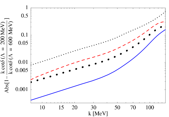
Figure 5: Logarithm of the cutoff variation of phase shifts between $\Lambda=200$ MeV and $\Lambda=600$ MeV as function of the centre-of-mass momentum. The short dashed, long dashed and solid line correspond respectively to LO, NLO and NNLO. The dots correspond to a “NNLO” calculation without the three-body force $H_{2}$.

The importance of isospin-violating effects can be estimated to be of higher order. In fact, the splitting between the ${}^{1}S_{0}$ scattering lengths between neutron-neutron ($a_{nn}$) and neutron-proton ($a_{np}$) can be estimated as $(1/a_{nn}-1/a_{np})/Q$, where $Q$ is the typical momentum in the system. Taking $Q\sim\sqrt{MB_{3}}$ this is a correction of about $2\%$, smaller than the cutoff variation we see at NNLO. For future high precision calculations, however, their inclusion is certainly required.

Unless otherwise stated, all calculations were performed with the cutoff at $600$ MeV. In the phase shift plots, we include the range of the NNLO result as the cutoff is varied between $200$ and $600$ MeV. Albeit it neglects other sources of error at low cutoffs, this is a reasonable estimate of the errors, especially at high momentum. A definite answer for the size of the errors, however, can only be given by a higher-order calculation. The lower limit of this variation was chosen to be of the order of the pion mass. The upper limit is rather arbitrary since beyond $\Lambda\approx 400$ MeV, the phase shifts are essentially cutoff independent. The phase shifts are cutoff independent up to the order the calculation is valid. This is demonstrated in the plot in Fig. 5, where we show the relative difference in $k\cot\delta$ caused by varying the cutoff between $\Lambda=200$ MeV and $\Lambda=600$ MeV at different orders. Two points are worth noticing. First, the cutoff variation decreases steadily as we increase the order of the calculation and is of the order of $(k/\Lambda)^{n},(\gamma/\Lambda)^{n}$, where $n$ is the order of the calculation and $\Lambda=200$ MeV is the smallest cutoff used. Second, the errors increase with increasing momentum, as one would expect from the fact that there are errors of order $(k/\Lambda)^{n}$. The slope does not change significantly as we go to higher orders due to the $(\gamma/\Lambda)^{n}$ terms. We also show in the same figure the same cutoff dependence of phase shifts but now calculated at NNLO without the three-body force $H_{2}$. It shows that not much improvement is obtained over the cutoff dependence of the NLO calculation, lending credence to the power counting discussed above.

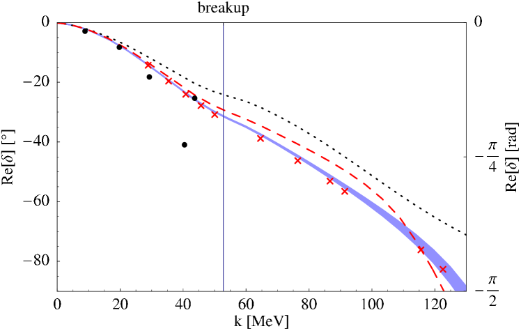
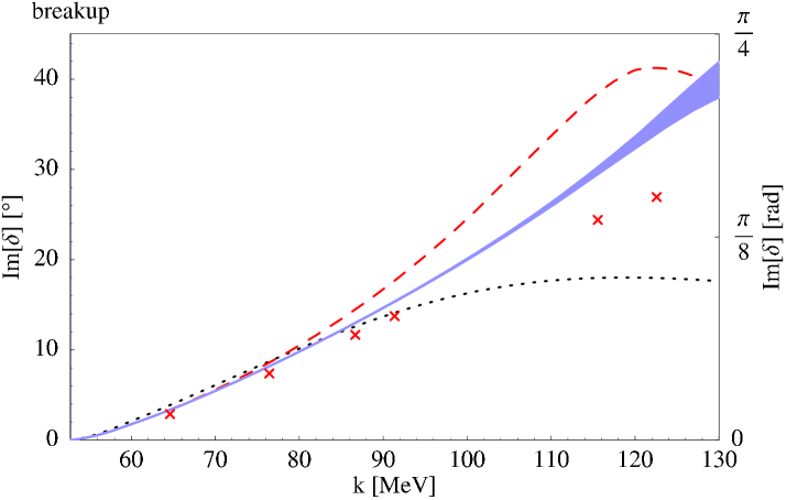
Figure 6: The neutron-deuteron ${}^{2}\mathrm{S}_{\frac{1}{2}}$ phase shift at LO (dotted line), NLO (dashed line) and NNLO (dark band). Top: Real part. Bottom: Imaginary part. The band in the NNLO curve corresponds to the change caused by a variation of the cutoff from $\Lambda=200$ MeV to $\Lambda=600$ MeV. The dots are from the only available direct phase shift analysis of the triton channel [15], which dates from 1967, and the crosses are the results obtained with the Argonne V18$+$Urbana IX two and three-body forces [16].

The phase shifts at LO, NLO and NNLO are shown in Fig. 6, together with the result of a phase shift analysis [15] and results from numerical calculations using the two-nucleon Argonne V18 potential and the Urbana IX three-body force [16] . The phase shifts converge steadily in the whole region of validity of our theory, up to centre-of-mass momenta of the order of $120$ MeV. At a momentum of the order of $\sqrt{MB_{3}}\sim 90$ MeV ($B_{3}$ the triton binding energy) the cutoff variation is of order of $24\%$, $12\%$ and $4\%$ respectively at LO, NLO and NNLO. Convergence by itself and to the results of the more sophisticated potential model calculation is achieved, albeit less pronounced in the imaginary part of the phase shift.

The comparison of our results with those obtained through potential models must however be done with care. Results obtained by the use of effective field theory have an universal validity in the following sense. Any model with the same experimental values for the low-energy constants as the ones we used to fix the low-energy constants of the effective theory, shares also the same prediction for other observables, up to the accuracy of the order of the EFT calculation. In our case, we expect thus that a model like the Argonne V$18$ two-body force complemented by the Urbana IX three-body force which predicts or fits the triton binding energy and low-energy two-body phase shifts, should give phase shifts agreeing with the effective theory result at the $4\%$, and this is indeed found. The agreement may disappear at higher order: The effective theory result will depend on low-energy constants determined by three-body observables that do not enter in the potential model determination and, through this information, can acquire higher accuracy. This is especially true when electroweak currents are considered.

A next-order calculation with an accuracy of about $1\%$ is straightforward and must include the mixing between the ${}^{2}\mathrm{S}_{\frac{1}{2}}$ and ${}^{4}\mathrm{D}_{\frac{1}{2}}$ partial waves, the contribution of two-body $p$-waves and isospin-breaking effects. However, although it does not involve any new unknown low-energy constants, it will not provide improved precision, since of the parameters used to fix our constants at the lower orders, the scattering length in the doublet $\mathrm{S}$ wave channel is not known with sufficient accuracy and would dominate the errors.

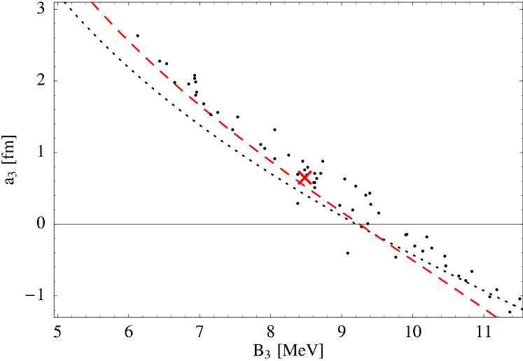
Figure 7: The Phillips line predicted at NLO. The dots correspond to the predictions for the triton biding energy and doublet scattering length in different models with the same two-body scattering lengths and effective ranges as inputs [24]. The dotted and dashed lines are the EFT results at LO and NLO, respectively. The cross is the experimental result.

The universality of the EFT predictions mentioned above is well illustrated by the Phillips line [25]. It is a well-known empirical fact that different models having the same low-energy two-body physics may have widely different three-body physics. The variation on the three-body physics is, however, correlated: One single three-body observable, say the triton binding energy, determines all the others, up to small corrections. In the EFT language, this is a reflection of the existence of the parameter $D_{0}$ (or $H_{0}$) already at leading order which is not determined by two-body physics but whose precise value at fixed cutoff must be determined from another three-body datum. Neither $D_{0}$ nor $\Lambda$ has an immediate physical significance, but once it is determined at a given cutoff, its cutoff dependence is fixed by (18). Therefore, as either of these parameters is varied as the other is kept fixed, the results of different potential models are reproduced. The basic physics leading to this effect was explained by Efimov in [6]. We here exemplify it by showing a plot of the predictions for the triton binding energy versus the doublet scattering length in a variety of models in Fig. 7, together with the EFT result at LO and NLO. The NLO result includes the (convenient but unnecessary) re-summation of higher order terms discussed above. We note that our NLO result is very similar to Efimov’s that was obtained by performing perturbation theory on the effective range [24].

V Conclusions and Outlook

We presented a simple scheme to classify at which order a given three-body force must be considered in an EFT approach to the few-body system at very low energies. These analytical considerations rest on the premise that a three-body force is included if and only if it is necessary to cancel cutoff dependences in the observables at a given order.

We compared the predictions of this scheme with its numerical implementation in the case of a NNLO calculation of the $nd$ scattering phase shifts in the ${}^{2}\mathrm{S}_{\frac{1}{2}}$ (triton) channel. We confirmed the well-known result that to LO and NLO, only one momentum dependent three-body force is necessary for cutoff independence, whose strength can be determined by the three-body scattering length. We found that one and only one new parameter enters at NNLO, namely the Wigner-$SU(4)$-symmetric three-body force with two derivatives. The one additional datum needed to fix it is the binding energy of the triton. Indeed, only the $SU(4)$-symmetric three-body forces are systematically enhanced over their contributions found from a naïve dimensional estimate, with a $2n$-derivative three-body force entering at the $2n$th order. On the way, we also propose a new, computationally convenient and simple scheme to perform higher order calculations in the three-body system by iterating a kernel to all orders, which has been expanded to the desired order of accuracy in the power counting.

The phase shifts thus calculated are in good agreement with a partial wave analysis and more sophisticated model computations. The result shows convergence.

Work under way includes the NNNLO calculation of the triton channel, its wave functions, the extension to ³He and the $pd$ channel, and the inclusion of electro-weak interactions. This will allow comparison to a plethora of data and lead to predictions in the range and to an accuracy relevant for astro-physical problems. Our scheme is clearly extendible to any EFT in which at least a partial re-summation of graphs at LO is necessary. More formal aspects of our method must also be addressed.

Appendix A Asymptotic Amplitude

In this appendix, we derive the asymptotic form of the half off-shell amplitudes quoted in the main text. Consider first the bosonic integral equation in (7) in the régime $\gamma,\sqrt{ME}\ll p\ll\Lambda$. For these values of $p$, the integral is dominated by values of $q$ of the order of $p$. We can then disregard the infrared scales $\gamma$ and $\sqrt{ME}$ as well as the term $H_{0}/\Lambda^{2}$ (assuming $H_{0}\approx 1$). The integral can be extended to infinity by adding a sub-leading piece. First dropping the inhomogeneous term, we find

$$t(p)=\frac{4}{\sqrt{3}\pi}\frac{1}{p}\int\limits_{0}^{\infty}\mathrm{d}q\;\;\ln\left(\frac{p^{2}+pq+q^{2}}{p^{2}-pq+q^{2}}\right)t(q)\;\;.$$ (36)

A Mellin transformation determines the solution to be a power law $t(p)\sim p^{s-1}$, where $s$ is determined by the equation

$$I(s)=1$$ (37)

with

$$I(s)=\frac{4}{\sqrt{3}\pi}\int\limits_{0}^{\infty}\mathrm{d}x\;\ln\left[\frac{x^{2}+x+1}{x^{2}-x+1}\right]\;x^{s-1}=\frac{8}{\sqrt{3}s}\frac{\sin(\frac{\pi s}{6})}{\cos(\frac{\pi s}{2})}\;\;.$$ (38)

The value of $s$ satisfying (37) with the largest real part dominates the asymptotics of $t(p)$. These values are the imaginary roots $s=\pm\mathrm{i}s_{0}\approx\pm\mathrm{i}\;1.0062\dots$. Because the inhomogeneous term in (7) behaves like $\sim 1/p^{2}$ in the asymptotic régime, it is consistent to ignore it compared to the asymptotics $p^{\pm\mathrm{i}s_{0}-1}$ of the homogeneous term. The overall normalisation of $t(p)$ can however not be determined by this analysis. What is perhaps more surprising is that the phase of the solution is not determined, either, since both $p^{\mathrm{i}s_{0}-1}$ and $p^{-\mathrm{i}s_{0}-1}$ are equally acceptable solutions. Sub-leading corrections to the asymptotics can be obtained in a similar fashion. For the corrections suppressed by one power of either $\gamma/p$ or $p\rho$ for instance, we insert $t(p)=p^{\mathrm{i}s_{0}-1}+8\gamma B_{-1}p^{\mathrm{i}s_{0}-2}+B_{1}\rho p^{\mathrm{i}s_{0}}$ in the equation

$$t(p)=\frac{2}{\pi}\int\limits_{0}^{\infty}\mathrm{d}q\;\frac{q}{p}\;\left(\frac{2}{\sqrt{3}}\frac{1}{q}+\frac{2}{3}\frac{\gamma}{q^{2}}+\frac{r}{2}\right)\ln\left(\frac{p^{2}+pq+q^{2}}{p^{2}-pq+q^{2}}\right)t(q)$$ (39)

and keep terms linear in $\gamma$ and $r$. Matching order by order, we find

$$B_{n}=\frac{\sqrt{3}}{4}\frac{I(\mathrm{i}s_{0}+n)}{1-I(\mathrm{i}s_{0}+n)}\;\;.$$ (40)

Taking real combinations of the solutions corresponding to $s_{0}$ and $-s_{0}$, we finally arrive at the result quoted in (23). Proceeding in a similar way, one can obtain this kind of correction to all orders, if necessary. We were however unable to find the sum of this series.

References

- [1] U. van Kolck, Prog. Part. Nucl. Phys. 43, 337 (1999) [nucl-th/9902015].
- [2] S.R. Beane, P.F. Bedaque, W.C. Haxton, D.R. Phillips and M.J. Savage, in “At the frontier of particle physics”, M. Shifman (ed.), World Scientific, 2001 [nucl-th/0008064].
- [3] P.F. Bedaque and U. van Kolck, nucl-th/0203055, to appear in Ann. Rev. Nucl. Part. Sci.
- [4] M. Rho, nucl-th/0202078.
- [5] H.A. Bethe, Phys. Rev. 76, 38 (1949).
- [6] V. Efimov, Nucl. Phys. A 362, 45 (1981); Phys. Rev. C 44, 2303 (1991); V. Efimov and E.G. Tkachenko, Phys. Lett. B 157, 108 (1985).
- [7] P.F. Bedaque and U. van Kolck, Phys. Lett. B 428, 221 (1998) [nucl-th/9710073].
- [8] P.F. Bedaque, H.-W. Hammer and U. van Kolck, Phys. Rev. C 58, R641 (1998) [nucl-th/9802057].
- [9] P.F. Bedaque and H.W. Grießhammer, Nucl. Phys. A 671, 357 (2000) [nucl-th/9907077].
- [10] F. Gabbiani, P.F. Bedaque and H.W. Grießhammer, Nucl. Phys. A 675, 601 (2000) [nucl-th/9911034].
- [11] G.S. Danilov, Sov. Phys. JETP 13, 349 (1961).
- [12] P.F. Bedaque, H.-W. Hammer and U. van Kolck, Phys. Rev. Lett. 82, 463 (1999) [nucl-th/9809025]; Nucl. Phys. A 646, 444 (1999) [nucl-th/9811046].
- [13] P.F. Bedaque, H.-W. Hammer and U. van Kolck, Nucl. Phys. A 676, 357 (2000) [nucl-th/9906032].
- [14] H.-W. Hammer and T. Mehen, Phys. Lett. B 516, 353 (2001) [nucl-th/0105072].
- [15] W.T.H. van Oers and J.D. Seagrave, Phys. Lett. B 24, 562 (1967).
- [16] A. Kievsky, S. Rosati, W. Tornow and M. Viviani, Nucl. Phys. A 607, 402 (1996); and private communication.
- [17] G.V. Skorniakov and K.A. Ter-Martirosian, Sov. Phys. JETP 4, 648 (1957).
- [18] F. Gabbiani, nucl-th/0104088.
- [19] R.A. Minlos and L.D. Faddeev, Sov. Phys. JETP 14, 1315 (1962).
- [20] A.N. Kolmogorov and V.N. Fomin, Elements of the Theory of Functions and Functional Analysis, Dover (1999).
- [21] E. Wigner, Phys. Rev. 51, 106 (1937).
- [22] J.H. Hetherington and L.H. Schick, Phys. Rev. B137, 935 (1965); R.T. Cahill and I.H. Sloan, Nucl. Phys. A165, 161 (1971); R. Aaron and R.D. Amado, Phys. Rev. 150, 857 (1966); E.W. Schmid and H. Ziegelmann, The Quantum Mechanical Three-Body Problem, Vieweg Tracts in Pure and Applied Physics Vol. 2, Pergamon Press (1974).
- [23] W. Dilg, L. Koester and W. Nistler, Phys. Lett. B 36, 208 (1971).
- [24] V. Efimov and E.G. Tkachenko, Few-Body Syst. 4, 71 (1988).
- [25] A.C. Phillips and G. Barton, Phys. Lett. B 28, 378 (1969).