The Density Matrix Renormalization Group Method for Realistic Large-Scale Nuclear Shell-Model Calculations

Abstract

The Density Matrix Renormalization Group (DMRG) method is developed for application to realistic nuclear systems. Test results are reported for ${}^{24}Mg$.

]

I Introduction

The nuclear shell model [1] is one of the most extensively used methods for a microscopic description of the nuclear structure. Within this approach, the nucleus is treated as an inert doubly–magic core and a number of valence nucleons, scattered by effective interaction over an active valence space consisting of at most a few major shells. Despite the enormous truncation inherent in this approach, the shell-model method as just described can still only be applied in very limited nuclear regimes, namely for those nuclei with a sufficiently small number of active nucleons or a relatively low degeneracy of the valence shells that are retained. The largest calculations that have been reported to date are for the binding energies of nuclei in the $fp$–shell through ${}^{64}Zn$ [2].

For heavier nuclei or nuclei farther from closed shells, one is forced to make further truncations in order to reduce the number of shell-model configurations to a manageable size. The most promising approach now in use is to truncate on the basis of Monte Carlo sampling[3]. In this way, it has recently proven possible to extend the shell model beyond the $fp$–shell to describe the transition from spherical to deformed nuclei in the Barium isotopes [4].

Nowadays, the Density Matrix Renormalization Group (DMRG) is recognized as a potentially promising tool for application to large– scale nuclear structure calculations. The method was initially developed and applied in the framework of low–dimensional quantum lattice systems [5] and then subsequently extended to finite Fermi systems to treat a pairing problem of relevance to ultrasmall superconducting grains [6]. This new approach, referred as the particle–hole (p–h) DMRG, was recently applied to a first test problem of some relevance to nuclear structure [7, 8, 9]. The application involved identical nucleons moving in a large single $j$–shell under the influence of a pairing plus quadrupole interaction with an additional single-particle energy term that split the shell into degenerate doublets. Comparing with the results of exact diagonalization, it was shown that the method leads to extremely accurate results for the ground state and for low–lying excited states without ever requiring the diagonalization of very large matrices. Furthermore, even when the problem was not amenable to exact solution, the method was seen to exhibit rapid exponential convergence. All of this has encouraged us to begin considering the application of the DMRG method in realistic shell-model calculations. We report here the results of our first attempt, a calculation for the nucleus ${}^{24}Mg$. Since exact shell model results exist for this nucleus, these calculations provide a meaningful test of the ability of the p-h DMRG method to work in realistic nuclear scenarios.

The paper is organized as follows. In Section II, we review the basic features of the p-h DMRG method. In Section III, we report results of calculations for a system of 40 like fermions in the $j=99/2$ shell, the starting point of our recent activities, and then present the first realistic application of the method to ${}^{24}Mg$. Finally in Section IV we summarize our principal conclusions and outline future directions of the project.

II The DMRG procedure

The basic idea of the DMRG method is to systematically take into account the physics of all single–particle levels. This is done by first taking into account the most important levels, namely those that are nearest to the Fermi surface, and then gradually including the others in subsequent iterations. At each step of the procedure, a truncation is implemented both in the space of particle states and in the space of hole states, so as to optimally take into account the effect of the most important states for each of these two subspaces of the problem. The calculation is carried out as a function of the number of particle and hole states that are maintained after each iteration, with the assumption that these numbers are the same. This parameter, which we will call $p$, is gradually increased and the results are plotted against it. Prior experience from other applications of the methodology suggests that the results converge exponentially with $p$. Thus, when we achieve changes with increasing $p$ that are acceptably small we simply terminate the calculation.

Since the p–h DMRG procedure has been discussed in some detail and generality in [9], here we just sketch the key steps and spell out how they are implemented specifically for ${}^{24}Mg$.

$1.$ We start by choosing the basis of the problem and the Fermi level for the nuclear system under consideration. ${}^{24}Mg$ can be considered as a double–magic ${}^{16}O$ core plus four valence neutrons and four valence protons, scattered over the orbits of the $sd$–shell. These are the $1d_{5/2}$, $2s_{1/2}$ and $1d_{3/2}$ levels, with degeneracies $6$, $2$ and $4$, respectively.

$2.$ The next step is to define the Hamiltonian of the system in the restricted set of active single-particle states. The Hamiltonian contains one– and two–body terms for like particles parts $H^{\tau}$, ${\tau}={\nu,\pi}$ and a two–body term for the proton–neutron part $H^{\nu\pi}$:

$$H=H^{\nu}+H^{\pi}+H^{\nu\pi}$$ (1)

where

$$H^{\tau} = \sum_{\alpha m}\epsilon_{\alpha m}a^{\tau\;\dagger}_{\alpha m}a^{\tau}_{\alpha m}$$ (2)

$$+ \frac{1}{4}\mathop{\sum_{\alpha_{1}m_{1},\alpha_{2}m_{2}}}_{\alpha_{3}m_{3},\alpha_{4}m_{4}}~{}\langle\alpha_{1}m_{1},~{}\alpha_{2}m_{2}|V|\alpha_{3}m_{3},~{}\alpha_{4}m_{4}\rangle$$ (4)

$$~{}~{}~{}~{}~{}~{}~{}~{}~{}~{}~{}~{}~{}~{}~{}~{}~{}\times a^{\tau\;\dagger}_{\alpha_{1}m_{1}}a^{\tau\;\dagger}_{\alpha_{2}m_{2}}a^{\tau}_{\alpha_{4}m_{4}}a^{\tau}_{\alpha_{3}m_{3}}$$

and

$$H^{\nu\pi} = \mathop{\sum_{\alpha_{1}m_{1},\alpha_{2}m_{2}}}_{\alpha_{3}m_{3},\alpha_{4}m_{4}}~{}\langle\alpha_{1}m_{1},~{}\alpha_{2}m_{2}|V|\alpha_{3}m_{3},~{}\alpha_{4}m_{4}\rangle$$ (6)

$$~{}~{}~{}~{}~{}~{}~{}~{}~{}~{}~{}~{}~{}~{}~{}~{}~{}\times a^{\nu\;\dagger}_{\alpha_{1}m_{1}}a^{\pi\;\dagger}_{\alpha_{2}m_{2}}a^{\nu}_{\alpha_{4}m_{4}}a^{\pi}_{\alpha_{3}m_{3}}\;.$$

Steps 1 and 2 together define the shell–model problem.

$3.$ The next step is to split up the set of multiply-degenerate spherical shell model levels into an appropriate ordered set of doubly-degenerate levels, which will be taken into account iteratively in the p–h DMRG procedure. In the case of ${}^{24}Mg$, the low–lying states are expected to be prolate deformed. This suggests that we first carry out a Hartree Fock calculation of ${}^{24}Mg$, using the chosen shell–model Hamiltonian, to define an appropriate prolate–deformed single–particle basis. The procedure, which is schematically illustrated in figure 1, leads to a set of doubly-degenerate levels, each having a definite value of the projection of angular momentum on the symmetry axis. For ${}^{24}Mg$, the Fermi energy both for neutrons and protons is between the first $3/2^{+}$ level and the second $1/2^{+}$ level.

FIG. 1.: Schematic illustration of the splitting of the model–space single–particle levels within the $sd$–shell into a set of doubly–degenerate levels by an axially–deformed Hartree–Fock calculation. The dashed line represents the Fermi energy ($E_{F}$), which separates the particle levels from the hole levels. Each doubly–degenerate level is labelled by its angular momentum projection on the intrinsic z-axis.

The Fermi surface splits the shell into two kind of states – the hole states below the Fermi level and the particle states above it. According to the p–h DMRG prescription we take first into account the particle and hole states closest to the Fermi surface and then gradually involve all of the others that are further away.

Note of course that for the nucleus ${}^{24}Mg$ there are four type of levels - particle and hole levels for neutrons and particle and hole levels for protons.

$4.$ We initialize the DMRG procedure by considering as active the lowest particle state above the Fermi surface and the highest hole state below. In the case of ${}^{24}Mg$, this means taking into account the $3/2^{+}_{1}$ hole level and the $5/2^{+}_{1}$ particle level, as they are the ones closest to the Fermi surface. For this set of particle states and hole states for protons and nucleons, we calculate the hamiltonian matrix and the matrices of all of its sub-operators, namely $a,\;aa,\;a^{{\dagger}}a,\;a^{{\dagger}}a^{{\dagger}}a$, and $a^{{\dagger}}a^{{\dagger}}aa$. Thus in a system of neutrons and protons we have four distinct blocks – neutron particle, proton particle, neutron hole and proton hole states.

$5.$  We then proceed to the first iteration by adding the next higher particle level and the next lower hole level. For ${}^{24}Mg$, these are the $1/2^{+}_{1}$ hole level and the $1/2^{+}_{2}$ particle level. In our calculations, we in fact add four levels, one for proton particles, one for proton holes, one for neutron particles and one for neutron holes.

We can express the particle and hole states in these enlarged spaces as

$$|\,I\,\rangle~{}=~{}|\,i\,\rangle_{old}\;|\,j\,\rangle_{new}~{},$$ (7)

where $|\,i\,\rangle_{old}$ refers to the $4$ particle (hole) states within the first iteration and $|\,j\,\rangle_{new}$ – to the $4$ new states from the additional level. Thus, each of these four blocks now contains 16 states.

To determine the matrix elements of the hamiltonian and all of its sub-operators in the proton–particle, proton–hole, neutron–particle and neutron–hole subspaces, we make use of the fact that all matrix elements in the old space are already known from the previous iteration while those coming from the new level are very simple to calculate. For example, the expectation values of the operators $a^{{\dagger}}a$ in the enlarged space looks like

$$\langle i,j|a^{\dagger}_{\alpha_{1}m_{1}}a_{\alpha_{2}m_{2}}|k,l\rangle =\langle i|a^{\dagger}_{\alpha_{1}m_{1}}a_{\alpha_{2}m_{2}}|k\rangle~{}\delta_{j,l}$$ (11)

$$+\langle j|a^{\dagger}_{\alpha_{1}m_{1}}a_{\alpha_{2}m_{2}}|l\rangle~{}\delta_{i,k}$$

$$+(-)^{n_{k}}\langle i|a^{\dagger}_{\alpha_{1}m_{1}}|k\rangle~{}\langle j|a_{\alpha_{2}m_{2}}|l\rangle$$

$$-(-)^{n_{k}}\langle i|a_{\alpha_{2}m_{2}}|k\rangle~{}\langle j|a^{\dagger}_{\alpha_{1}m_{1}}|l\rangle~{},$$

where $n_{i}$ is the number of particles in state $|i\rangle$.

$6.$  The next step is to couple the states in the four blocks. In doing this, we only keep those product states in which the total number of particles for protons equals the total number of holes for protons and the same for neutrons (to make the theory particle number conserving) and in which the total angular momentum projection of the system is $M=0$. We will call the number of such coupled states $N$. Note that it is significantly less than $16\times 16$ because of the above restrictions on the number of particles and holes and on the total $M$ value. We then calculate the matrix elements of the full hamiltonian eqs.(1,4,6) in this product basis (often called the superblock), making use of the fact that we know the matrix elements of the hamiltonian and all its sub-operators separately in the particle and hole spaces for protons and neutrons.

$7.$  Next we diagonalize the superblock hamiltonian:

$$H|\Psi_{\alpha}\rangle=E_{\alpha}|\Psi_{\alpha}\rangle~{},$$ (13)

with

$$|\Psi_{\alpha}\rangle=\mathop{\sum_{i^{\nu}_{p},j^{\nu}_{h}}}_{{k^{\pi}_{p},l^{\pi}_{h}}}\Psi^{(\alpha)}_{ijkl}|i^{\nu}_{p}\rangle|j^{\nu}_{h}\rangle|k^{\pi}_{p}\rangle|l^{\pi}_{h}\rangle~{}.$$ (14)

Note that the sums go over the all $16$ states in the respective enlarged particle and hole blocks for protons and neutrons.

$8.$ The next step is to truncate to the optimum $p$ states in the four blocks, optimum in the sense that the states we retain provide the optimum approximation to the system prior to truncation.

If $p$ is greater than $16$, no truncation is required and we simply continue to the next iteration, adding the next levels for particles and holes.

If $p$ is less than $16$, we perform the optimized truncation in the following way. If we want to optimize the description of the L lowest eigenstates of the hamiltonian, we have to construct the mixed density matrices to these L eigenstates in the four blocks - particles and holes ($p,h$) for protons and neutrons($\tau=\nu,\pi$). For example for neutrons they are:

$$\rho^{\nu\;p}_{ii^{\prime}}=\frac{1}{L}\sum_{\alpha=1,L}\sum_{j,k,l=1,4p}\Psi^{\alpha}_{ijkl}{\Psi^{\alpha*}_{i^{\prime}jkl}}~{},$$ (15)

$$\rho^{\nu\;h}_{jj^{\prime}}=\frac{1}{L}\sum_{\alpha=1,L}\sum_{i,k,l=1,4p}\Psi^{\alpha}_{ijkl}{\Psi^{\alpha*}_{ij^{\prime}kl}}~{}.$$ (16)

We then diagonalize all four of these density matrices, each of which is of dimension $4p$:

$$\rho^{\tau p}\left|\,u^{\beta}\,\right\rangle_{\tau p}~{}=~{}\omega^{\tau p}_{\beta}~{}\left|\,u^{\beta}\,\right\rangle_{\tau p}~{},$$ (17)

$$\rho^{\tau h}\left|\,u^{\beta}\,\right\rangle_{\tau h}~{}=~{}\omega^{\tau h}_{\beta}~{}\left|\,u^{\beta}\,\right\rangle_{\tau h}~{}.$$ (18)

Those $p$ eigenstates with the largest eigenvalues provide the optimum approximation to the set of $L$ states that were targeted in constructing the corresponding mixed density matrix.

$9.$ The final step of the iteration is to transform the matrices of all needed combinations of creation and annihilation operators in the four blocks from the $4p$–dimensional spaces to the optimal $p$–dimensional truncated spaces.

$10..$ The next step is to proceed to the next iteration by adding the next set of levels and following steps $5-9$. We continue to add one level from each block, until one (or more) of them is exhausted. From that point on, we only add levels from the remaining blocks, and only carry out the optimized truncation for them. The procedure ends when all states of the four block are exhausted. Note that in the case of ${}^{24}Mg$, there are a total of three iterations. In the first iteration, both particle and hole levels are added. In subsequent iterations only particle levels are added.

III Results

Before presenting the results of our realistic calculations for ${}^{24}Mg$ we first return for a moment to the single-j shell–model system discussed in [8, 9]. The largest calculations we have so far carried out is for a system of 40 particles occupying a single $j=99/2$ orbit and interacting via pairing plus quadrupole interaction with an additional one-body term to split the degeneracy of the orbit.

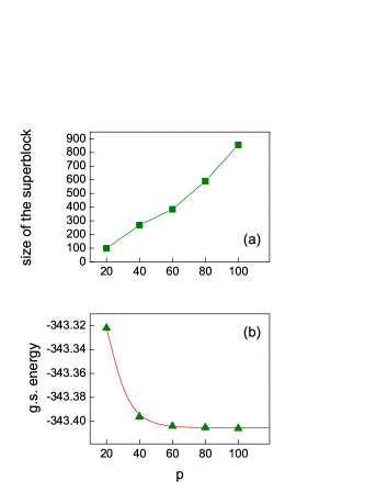
FIG. 2.: The maximum size of the superblock (a) and the ground-state energy (b) for a system of 40 identical nucleons in a single $j=99/2$ orbit interacting via pairing plus quadrupole Hamiltonian. An exponential fit to these results is also plotted.

In this case, the exact calculation would involve a hamiltonian matrix of dimension $3.84007\times 10^{25}$, obviously much too large to treat without dramatic truncation. In figure 2, we display the largest size of the hamiltonian matrix we had to diagonalize and the ground state energy of the system as a function of $p$. It is seen that while the energy of the ground state follows a steep exponential trend, the size of the superblock increases linearly. This gives us hope that we can treat realistic nuclear systems accurately using the DMRG strategy, while keeping the size of the matrices manageable.

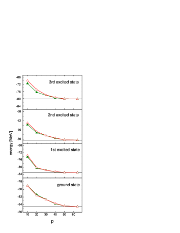
FIG. 3.: The energy of the ground state and of the three lowest excited states for ${}^{24}Mg$. The open triangles are the results when only the ground state is targeted in the optimization procedure; the solid triangles refer to calculations when the lowest four states of the system are all targeted simultaneously.

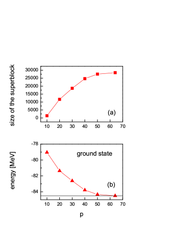
FIG. 4.: The maximum size of the superblock $(a)$ and the energy of the ground state $(b)$ for ${}^{24}Mg$, when only the ground state is targeted in the optimization procedure.

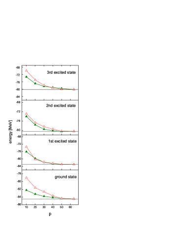
FIG. 5.: The energy of the ground state and of the three lowest excited states for ${}^{24}Mg$, when only the ground state is targeted in the optimization procedure. The solid triangles refer to calculations in the deformed HF-basis and the open triangles to calculations in the spherical basis.

The first realistic p-h DMRG calculations we performed were for ${}^{24}Mg$. As noted earlier, this system is assumed in the shell model to be a ${}^{16}O$ core plus four valence neutrons and four valence protons in the $sd$–shell. We have used the Wildenthal’s USD interaction [10, 11]. The main reason for considering this nucleus first is that the shell–model problem for ${}^{24}Mg$ can be solved exactly. The size of the Hilbert space in the $m$–scheme is $28,503$ for which the Hamiltonian matrix can be treated using the Lanczos algorithm.

In these calculations, we have considered two possible strategies for defining the order of doubly–degenerate levels to include in the iterative DMRG procedure. As discussed in Section II, the most appropriate strategy is to use an axially-symmetric HF calculation to define the states and to calculate all matrix elements in that deformed basis. A simpler strategy is to use the HF procedure to tell us the order in which to fill the $|m|$ values, but to still carry out the calculation in the spherical basis. For ${}^{24}Mg$, this would correspond to an ordering of levels such that the $d_{5/2~{}1/2}$ is lowest, followed by the $d_{5/2~{}3/2}$, the $d_{3/2~{}1/2}$, the $d_{5/2~{}5/2}$, the $s_{1/2~{}1/2}$ and then finally the $d_{3/2~{}3/2}$. The latter strategy should converge more slowly, but is simpler to implement and less time consuming.

We first show the results using a spherical shell–model basis, but with a slightly different ordering of levels than above, namely $d_{5/2~{}1/2}$, $d_{5/2~{}3/2}$, $d_{5/2~{}5/2}$, $s_{1/2~{}1/2}$, $d_{3/2~{}1/2}$ and $d_{3/2~{}3/2}$ . Figure 3 shows the ground state energy and the energy of the first three excited states as a function of the number of states $p$ kept for each block during the DMRG procedure. The exact results are represented by a straight line. For $p=64$ the whole shell–model space is exhausted and the exact results are reproduced. Results for two set of calculations are displayed – when just the ground state is taken into account in the reduced density matrices (eqs.[16]) and when the lowest four states are targeted simultaneously. A first look at this figure tells us that, contrary to our expectations, the exponential conversion of the energy with $p$ is not especially rapid, neither for the ground state nor for the excited states. From figure 4, we see that an accuracy of $0.2\%$ for the ground state energy requires $p=50$, where $97\%$ of the shell-model states are taken into account. Moreover the size of the superblock increases exponentially with $p$, contrary to the single–j case where the dependence was linear.

Going back to figure 3, we also see that including excited states in defining the reduced density matrices improves slightly the description of the energy of the excited states without significantly changing the ground state energy. Moreover once $p$ becomes large enough, there is no discernable difference between the two sets of results.

Next we consider what happens when the calculations are carried out in the deformed Hartree–Fock single–particle basis. Figure 5 compares the results obtained for the ground state energy and the energies of the three lowest excited states as a function of $p$ in the spherical basis (the open triangles) and in the HF–basis (the full triangles). Is is seen that there is a significant improvement in the results, especially for the ground state energy, for small values of $p$. For $p$ values larger then $40$, however, use of the HF–basis is of no great value. Most importantly, in neither case can we achieve a high level of accuracy without including a large fraction of the full Hilbert space.

IV Closing Remarks

In this paper, we presented results of the first p-h DMRG calculations carried out for a realistic nuclear system. We considered the nucleus ${}^{24}Mg$, for which exact shell–model calculations assuming an inert ${}^{16}O$ core and 8 valence nucleons in the $sd$–shell have been reported. Our calculations used the same Wildenthal $USD$–interaction as the exact calculations, so as to permit a meaningful test of the DMRG method.

The results show that, independent of the single–particle basis used, the exponential convergence for the ground state energy and for the energies of the lowest excited states is fairly slow. To get accurate results we must include almost the complete space.

The first question to be addressed in the future is whether these results are a consequence of the very small shell–model space for ${}^{24}Mg$. We will thus consider the somewhat larger, but still exactly solvable, problem of ${}^{48}Cr$.

The next step after that is to include sweeps in the DMRG method, whereby we go through the set of levels several times [5]. While this will no doubt lead to better accuracy of the method, it still remains to be seen whether it will lead to very accurate results with a relatively small number of states kept. If so, we will then turn to the ultimate goal of this project, to use the method to treat larger–scale and more challenging nuclear structure problems.

- [1] See, e.g., K. Heyde, The Nuclear Shell Model (Springer-Verlag, Berlin, 1990).
- [2] E. Caurier , Phys. Rev. C 59, 2033 (1999).
- [3] M. Honma, T. Mizusaki and T. Otsuka, Phys. Rev. Lett. 77, 3315 (1996).
- [4] M. Shimizu, T. Otsuka, T. Mizusaki, and M. Honma, to be published in Phys. Rev. Lett.
- [5] S. R. White, Phys. Rev. Lett. 69, 2893 (1992); Phys. Rev. B 48,10345 (1993); Phys. Rep. 301, 187 (1998).
- [6] J. Dukelsky and G. Sierra, Phys. Rev. Lett. 83, 172 (1999); and Phys. Rev. B61, 12302 (2000).
- [7] J. Dukelsky and S. Pittel, Phys.Rev. C63 (2001) 061303.
- [8] S.S. Dimitrova, S. Pittel, J. Dukelsky, and M.V. Stoitsov, in Procc. 20. International Workshop on Nuclear Theory, (Rila, Bulgaria, June 11-16, 2001), Notre-Dame, Indiana, pp. 2001.
- [9] J. Dukelsky, S. Pittel, S. S. Dimitrova, and M. V. Stoitsov, Phys.Rev. C65 (2002) 054319.
- [10] B.H.Wildenthal, Prog. Part. Nucl. Phys. 11, 5 (1984).
- [11] B.A.Brown and. B.H.Wildenthal, Annu. Rev. Nucl. Part. Sci 38, 292 (1988).