[

In-Band and Inter-Band $B(E2)$ Values within the Triaxial Projected Shell Model

Abstract

The Triaxial Projected Shell Model (TPSM) has been successful in providing a microscopic description of the energies of multi-phonon vibrational bands in deformed nuclei. We report here on an extension of the TPSM to allow, for the first time, calculations of $B(E2)$ values connecting $\gamma$- and $\gamma\gamma$-vibrational bands and the ground state band. The method is applied to ^166,168Er. It is shown that most of the existing $B(E2)$ data can be reproduced rather well, thus strongly supporting the classification of these states as $\gamma$-vibrational states. However, significant differences between the data and the calculation are seen in those $B(E2)$ values which involve odd-spin states of the $\gamma$-band. Understanding these discrepancies requires accurate experimental measurements and perhaps further improvements of the TPSM.

]

Recently two-phonon $\gamma\gamma$-vibrational bands have been identified in a number of nuclei [1, 2, 3], where pronounced anharmonicities have been observed in the vibrational spectrum. A microscopic description of the energies and transition probabilities of two-phonon vibrational excitations remains a challenge to nuclear models. The Triaxial Projected Shell Model [4, 5] is a new microscopic, fully quantum-mechanical model with a unified treatment of the vibrational and rotational states. In the TPSM approach, one introduces triaxiality in the deformed basis and performs exactly three-dimensional angular momentum projection [4]. In this way, the deformed vacuum state is much enriched by allowing all possible $K$-components. Diagonalization mixes these components, and various excited bands emerge [5] besides the ground state (g.s.) band ($K=0$). The excited $K=2$ band describes the one-phonon $\gamma$-vibrational band; and the excited band with $K=4$ accounts for the two-phonon $\gamma\gamma$-band. The observed anharmonicities in the energies of multi-phonon vibrational bands occur quite naturally from the TPSM without including additional ingredients in the model [5]. The TPSM has recently been applied also to the study of transition quadrupole moments in the g.s. bands of $\gamma$-soft nuclei and the magnetic dipole properties of the $\gamma$-vibrational states [6, 7]. However, in-band and inter-band E2-transitions, which are important quantities in supporting classification of states, have not been studied yet.

The purpose of this paper is to report a new extension of the TPSM which allows the calculation of $B(E2)$ values for transitions connecting the g.s. band, the single $\gamma$, and double $\gamma\gamma$ vibrational bands. We have searched the entire rare-earth region for experimental inter-band $B(E2)$ values that allow a comparison with our calculations. Data on absolute $B(E2)$ values are sparse and only in few cases they are known for more than one or two members of the $\gamma$-band. In this paper we study $B(E2)$ values for ^166,168Er, which are the best cases. These nuclei exhibit well established double-phonon excitations [2, 3]. ¹⁶⁸Er is one of the most extensively studied nuclei in this mass region with several measured $B(E2)$ values for members of the $\gamma$-band [8] and $\gamma\gamma$-band [3].

In the TPSM, one calculates the $\gamma$-vibrational states by building a shell model space truncated in a triaxially deformed basis. This is done by an exact three-dimensional angular-momentum projection of the $\gamma$-deformed Nilsson + BCS basis $\left|\Phi\right\rangle$. The Nilsson Hamiltonian is:

$$\hat{H}=\hat{H}_{0}-\frac{2}{3}\hbar\omega\left[\epsilon\hat{Q}_{0}+\epsilon^{\prime}\frac{\hat{Q}_{+2}+\hat{Q}_{-2}}{\sqrt{2}}\right]$$ (1)

where $\hat{H}_{0}$ is the spherical single-particle Hamiltonian with inclusion of the appropriate spin-orbit forces parameterized by Nilsson et al. [9]. The axial and the triaxial parts of the Nilsson potential in Eq. (1) contain the parameters $\epsilon$ and $\epsilon^{\prime}$ respectively, which are related to the conventional triaxiality parameter by $\gamma=\tan(\frac{\epsilon^{\prime}}{\epsilon})$. The rotational invariant two-body Hamiltonian

$$\hat{H}=\hat{H}_{0}-\frac{\chi}{2}\sum_{\mu}\hat{Q}_{\mu}^{+}\hat{Q}_{\mu}-G_{M}\hat{P}^{+}\hat{P}-G_{Q}\sum_{\mu}\hat{P}_{\mu}^{+}\hat{P}_{\mu}$$ (2)

is diagonalized in the TPSM basis:

$\left\{\hat{P}_{MK}^{I}\left|\Phi\right\rangle,0\leq K\leq I\right\}$. The solutions take the form

$$\left|\Psi^{\sigma}_{IM}\right\rangle=\sum_{0\leq K\leq I}f^{\sigma}_{IK}\hat{P}_{MK}^{I}\left|\Phi\right\rangle,$$ (3)

where $\sigma$ specifies the states with the same angular momentum $I$. The strength of the monopole and quadrupole pairing forces is set by $G_{M}$ and $G_{Q}$ in Eq. (2), where $G_{M}=\left[G_{1}\pm G_{2}\frac{N-Z}{A}\right]/A$ with $"+"$ for protons and $"-"$ for neutrons. We use $G_{1}=20.12$, $G_{2}=13.13$ and $G_{Q}=0.16G_{M}$, which are the same values used in previous calculations [4, 5, 10]. The $QQ$-force strength $\chi$ is determined such that it holds a self-consistent relation with the quadrupole deformation $\epsilon$ [10].

Once the Hamiltonian is diagonalized in the TPSM basis, the eigenfunctions are used to calculate the electric quadrupole transition probabilities

$\displaystyle B(E2:(I_{i},K_{i})\rightarrow(I_{f},K_{f}))=\frac{1}{2I_{i}+1}\left|\left\langle\Psi^{K_{f}}_{I_{f}}||\hat{Q}_{2}||\Psi^{K_{i}}_{I_{i}}\right\rangle\right|^{2}$

between an initial state $(I_{i},K_{i})$ and a final states $(I_{f},K_{f})$. The explicit expression for the reduced matrix element in the projected basis can be found in Ref. [6]. Note that we now use $K$ instead of $\sigma$ to specify states with the same angular momentum $I$. According to Eq. (3), $K$ is not a good quantum number. However, it has been shown [5] that in these well-deformed nuclei, $K$-mixing is rather weak. Thus, we use $K$ to denote bands keeping the familiar convention. In the calculation, we use the standard effective charges of 1.5$e$ for protons and 0.5$e$ for neutrons.

In the present calculation , the parameters $\epsilon$ and $\epsilon^{\prime}$ are considered as adjustable. For the deformation parameter $\epsilon$ the experimental value 0.320 [11] is used, which means it is chosen such that the experimental value of $B(E2:2^{+}_{K=0}\rightarrow 0^{+}_{K=0})$ is approximately reproduced. In previous applications, the calculated deformation parameters [12] were used, which means in the present case $\epsilon=0.273$. Besides giving a better scale for the $B(E2)$ values, the use of the experimental $\epsilon$ slightly better reproduces the energy levels [13]. Except for the overall scale, $B(E2)$ values are not very sensitive to the moderate changes of $\epsilon$, in particular the $B(E2)$ values of the $\gamma$-vibrational states. The triaxiality parameter $\epsilon^{\prime}$ is chosen so that the calculated energy of the $K=2$ band-head reproduces the measured value. For ¹⁶⁸Er, we find $\epsilon^{\prime}=0.125$.

The experimental and calculated energies for ¹⁶⁸Er are compared in Fig. 1. It can be seen that all the energy levels in the g.s. band, the $\gamma$-band, and the $K=4$ $\gamma\gamma$-band are well described within the TPSM. Without introducing additional ingredients, the model gives anharmonicities in the energies of the $\gamma\gamma$ vibrational bands, which are bigger in comparison with experiment.

The calculated $B(E2)$ values from the TPSM are not far from the ones for a rotor coupled to a harmonic vibrator (see e.g. [15]). This familiar limit is included in Fig. 2, where the $B(E2)$ values for transitions within the $\gamma$-band of ¹⁶⁸Er are compared with experimental data from Ref.[2, 8, 14, 16]. Table I and Fig. 2 compare the complete set of $B(E2)$ values. Except for some particular transitions that we shall discuss below, most of the theoretical $B(E2)$ values appear to agree with the measured values. In general, the in-band transition probabilities are two order of magnitude stronger than the inter-band transitions. The $B(E2)$ transitions from the $\gamma\gamma$-band are quite well reproduced in TPSM.

There may be a discrepancy between the calculated and measured $B(E2)$ values involving the odd-spin $3^{+}_{K=2}$ state of the $\gamma$-band. For example, the experimental $B(E2:3^{+}_{K=2}\rightarrow 2^{+}_{K=2})$ value is $>12$ $W.u.$ while the calculated value from the TPSM gives 408 $W.u.$ Similarly, the calculated $B(E2:3^{+}_{K=2}\rightarrow 2^{+}_{K=0})$ is $5$ $W.u.$, which is by an order of magnitude larger than the experimental lower limit of $>0.2$ $W.u$. The $B(E2:3^{+}_{K=2}\rightarrow 4^{+}_{K=0})$ is also an order of magnitude off the limit. The experimental values are lower limits because there is only an upper limit known for the lifetime [17] of the $3^{+}_{K=2}$ state. The $3^{+}_{K=2}$ state is described as a rotational state built on a $\gamma$-vibration. Therefore all models that use this picture will give a large probability for the $3^{+}_{K=2}\rightarrow 2^{+}_{K=2}$ transition. Accordingly, the large experimental $B(E2)$ value for the $4^{+}_{K=2}\rightarrow 2^{+}_{K=2}$ transition in the $\gamma$-band is very well described by the theory. Clearly a more accurate lifetime measurement of the $3^{+}_{K=2}$ state ¹⁶⁸Er is desirable in order to settle the question, whether there is a discrepancy between theory and experiment for transitions involving the odd-spin states or not.

One expects that collective levels with energies larger than the pairing gap $2\Delta$ are to some extent mixed with the two-quasiparticle excitations. The present calculations do not explicitly include excited quasiparticle configurations based on the $\gamma$-deformed basis. The experimental $B(E2)$ values are well reproduced for states that are expected to weakly mix with two-quasiparticle excitations. The only exception is the $3^{+}_{K=2}$ state, which is inconclusive. The states of the $\gamma\gamma$-band lie in the energy region where mixing with the two-quasiparticle states should become important. The calculated $B(E2)$ value for the $4^{+}_{K=4}\rightarrow 2^{+}_{K=2}$ transition is about four times and the one for the $4^{+}_{K=4}\rightarrow 3^{+}_{K=2}$ is about three times larger than in experiment. A substantial admixture of a two-quasiparticle states into the collective $\gamma\gamma$-vibration would reduce this $B(E2)$ value. Such a mixing may also account for the deviation between the experimental and calculated energies of the $\gamma\gamma$-vibration. The other significant discrepancy is associated with the $8^{+}_{K=2}$ level at $1625$ $keV$. The calculated $B(E2:8^{+}_{K=2}\rightarrow 6^{+}_{K=2})$ is 323 $W.u.$, which is about 4.5 times larger than the measured value. At this excitation energy and angular momentum, single particle excitations are expected mix with the collective states, leading to crossing between collective and two-quasiparticle bands. The $B(E2:8^{+}_{K=2}\rightarrow 10^{+}_{K=0})$ shown in Table I has a calculated value of 1.4 $W.u$. One would expect that the single particle effects will tend to further reduce this number, but the experimental value is $120\pm 50$ $W.u.$ The reason for the increased collectivity is not clear. This is an indication that at high spins the $\gamma$-band behaves differently from what is expected for a collective excitation.

We also calculated energies and B(E2) values for ¹⁶⁶Er. Here, we use $\epsilon=0.324$ [11] and $\epsilon^{\prime}=0.126$; all other parameters are the same as for ¹⁶⁸Er. The experimental data for the g.s. band, $\gamma$-band energy, life times and intensities of the $\gamma$ transitions of interest are taken from Ref. [3, 18]. The data for the $\gamma\gamma$-band is taken from Ref. [3]. Fig. 3 and Table II show the level energies for the g.s., $\gamma$-, $\gamma\gamma$-bands, and the B(E2) values for ¹⁶⁶Er, respectively.

This calculation leads to the same conclusion as in the ¹⁶⁸Er case: The TPSM describes the energies of the g.s. band and the $\gamma$-band well. The energies of the $\gamma\gamma$-band are reproduced quite well for ¹⁶⁶Er (see Fig. 3). In fact, one can argue that the $4^{+}_{K=4}$ state wave function in ¹⁶⁶Er is more collective than in ¹⁶⁸Er because the $B(E2)_{TPSM}$ value of $12$ $W.u.$ is closer to the experimental one of $7.4$ $W.u$. For the transitions from the odd-spin states of the $\gamma$-band there is a similar inconclusive situation as in ¹⁶⁸Er. In ¹⁶⁶Er, only the upper limit on the lifetime of the $5^{+}_{K=2}$ state is known experimentally. The calculated $B(E2:5^{+}_{K=2}\rightarrow 3^{+}_{K=2})$ value is $223$ $W.u.$ while the experimental limit is $>14$ $W.u$. There is an order of magnitude difference between the theoretical $B(E2:5^{+}_{K=2}\rightarrow 4^{+}_{K=0})$ and $B(E2:5^{+}_{K=2}\rightarrow 6^{+}_{K=0})$ values and the experimental limits.

In conclusion, the Triaxial Projected Shell Model has been successful in describing the experimental level energies for the g.s., the $\gamma$, and the $\gamma\gamma$-bands with their inherent anharmonicities. We have calculated for the first time, $B(E2)$ values for inter-band transitions between the g.s., $\gamma$-, and $\gamma\gamma$-bands in ^166,168Er. Most of the calculated $B(E2)$ values well agree with the available experimental data. Only lower limits for $B(E2)$ values associated with the odd-spin members of the $\gamma$-band can be derived from the available data. More accurate lifetime measurements are necessary for a stringent test of the theory. The deviations between calculated and experimental $B(E2)$ values seem to point to the inclusion of two-quasiparticle admixtures in the collective excitations. Hence, it appears necessary to explicitly include excited quasi-particle configurations into the Triaxial Projected Shell Model in order to achieve an understanding of the nature of vibrational states in deformed nuclei where fragmentation of collectivity among quasiparticle excitations is expected to play an important role.

Research on this topic was supported by the National Science Foundation under the contract 99-01133 and the Department of Energy under the grant DE-FG02-95ER40934.

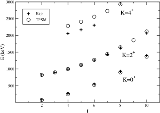
FIG. 1.: The energies [2, 8, 14] of levels within the g.s., $\gamma$-, and $\gamma\gamma$-bands in ¹⁶⁸Er compared with those calculated within the TPSM as a function of spin I.

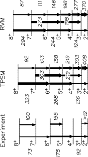
FIG. 2.: Comparison of experimental in-band B(E2) values for the K${}^{\pi}=2^{+}$ $\gamma$-band with calculations of the TPSM and the RVM in ¹⁶⁸Er. The thickness of the arrows is proportional to the magnitude of the transition probabilities in W.u.

TABLE I.: Comparison of all known experimental in-band and inter-band $B(E2)$ values (associated errors in parenthesis) and calculated ones in $W.u.$ for ¹⁶⁸Er. K=4⁺ lifetimes from Ref.[2], K=0⁺, and K=2⁺ lifetimes and B(E2) values from Ref.[8] and all the references therein.
^∗ B(E2) value from Ref.[16]; the calculated axial rotor value is $336$ $W.u$.
^∗∗ B(E2) values calculated from lifetimes in Ref.[2].

$(I,K)_{i}\rightarrow(I,K)_{f}$	$B(E2)_{\exp}(W.u.)$	$B(E2)_{TPSM}(W.u.)$
$(2,0)_{i}\rightarrow(0,0)_{f}$	207 (6)	228.6
$(4,0)_{i}\rightarrow(2,0)_{f}$	318 (12)	326.9
$(6,0)_{i}\rightarrow(4,0)_{f}$	440* (30)	361.2
$(8,0)_{i}\rightarrow(6,0)_{f}$	350 (20)	380.0
$(10,0)_{i}\rightarrow(8,0)_{f}$	302 (21)	393.0
$(2,2)_{i}\rightarrow(0,0)_{f}$	4.80 (17)	2.7
$(2,2)_{i}\rightarrow(2,0)_{f}$	8.5 (4)	4.5
$(2,2)_{i}\rightarrow(4,0)_{f}$	0.62 (4)	0.3
$(3,2)_{i}\rightarrow(2,0)_{f}$	$>0.19$	4.9
$(3,2)_{i}\rightarrow(4,0)_{f}$	$>0.13$	2.7
$(4,2)_{i}\rightarrow(2,0)_{f}$	1.7 (4)	1.3
$(4,2)_{i}\rightarrow(4,0)_{f}$	8.7 (18)	5.5
$(4,2)_{i}\rightarrow(6,0)_{f}$	1.13 (25)	0.7
$(5,2)_{i}\rightarrow(4,0)_{f}$		3.9
$(5,2)_{i}\rightarrow(6,0)_{f}$		3.7
$(6,2)_{i}\rightarrow(4,0)_{f}$	0.78 (19)	0.8
$(6,2)_{i}\rightarrow(6,0)_{f}$	6.4 (16)	5.7
$(6,2)_{i}\rightarrow(8,0)_{f}$	2.4 (7)	1.1
$(7,2)_{i}\rightarrow(6,0)_{f}$		3.3
$(7,2)_{i}\rightarrow(8,0)_{f}$		4.4
$(8,2)_{i}\rightarrow(6,0)_{f}$	1.3 (6)	0.5
$(8,2)_{i}\rightarrow(8,0)_{f}$	1.8 (8)	5.7
$(8,2)_{i}\rightarrow(10,0)_{f}$	120 (50)	1.4
$(4,4)_{i}\rightarrow(2,2)_{f}$	3.4 (19)	11.9
$(4,4)_{i}\rightarrow(3,2)_{f}$	2.2 (13)	7.1
$(4,4)_{i}\rightarrow(4,2)_{f}$	1.7** (9)	2.7
$(4,4)_{i}\rightarrow(5,2)_{f}$	0.7** (3)	0.6
$(4,4)_{i}\rightarrow(6,2)_{f}$	2.0 (13)	0.1
$(5,4)_{i}\rightarrow(3,2)_{f}$	5 (5)	7.7
$(5,4)_{i}\rightarrow(4,2)_{f}$	4 (3)	8.6
$(5,4)_{i}\rightarrow(5,2)_{f}$	1.8 (15)	4.6
$(5,4)_{i}\rightarrow(6,2)_{f}$	0.8 (7)	1.3
$(5,4)_{i}\rightarrow(7,2)_{f}$	7 (6)	0.2

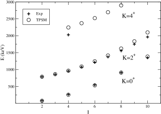
FIG. 3.: The energies [18] of levels within the g.s., $\gamma$-, and $\gamma\gamma$-bands in ${}^{166}Er$ compared with calculated values from the TPSM as a function of spin I. .

TABLE II.: Comparison of all known experimental in-band and inter-band $B(E2)$ values (associated errors in parenthesis) and calculated ones in $W.u.$ for ¹⁶⁶Er.
^∗ $B_{exp}(E2)$ is calculated as an upper limit assuming 100% E2.
^∗∗ Data from Ref.[3].

$(I,K)_{i}\rightarrow(I,K)_{f}$	$B(E2)_{exp}(W.u.)$	$B(E2)_{TPSM}(W.u.)$
$(2,0)_{i}\rightarrow(0,0)_{f}$	214 (10)	231.6
$(4,0)_{i}\rightarrow(2,0)_{f}$	311 (20)	331.3
$(6,0)_{i}\rightarrow(4,0)_{f}$	347 (45)	366.2
$(8,0)_{i}\rightarrow(6,0)_{f}$	365 (50)	385.5
$(10,0)_{i}\rightarrow(8,0)_{f}$	371 (46)	399.1
$(3,2)_{i}\rightarrow(2,2)_{f}$		414.0
$(4,2)_{i}\rightarrow(2,2)_{f}$		137.8
$(4,2)_{i}\rightarrow(3,2)_{f}$		306.8
$(5,2)_{i}\rightarrow(3,2)_{f}$	$>14$	222.0
$(5,2)_{i}\rightarrow(4,2)_{f}$	$>18$*	221.6
$(2,2)_{i}\rightarrow(0,0)_{f}$	5.5 (4)	2.8
$(2,2)_{i}\rightarrow(2,0)_{f}$	9.7 (7)	4.7
$(2,2)_{i}\rightarrow(4,0)_{f}$	0.67 (5)	0.3
$(5,2)_{i}\rightarrow(4,0)_{f}$	$>0.4$	3.8
$(5,2)_{i}\rightarrow(6,0)_{f}$	$>0.6$	4.1
$(4,4)_{i}\rightarrow(2,2)_{f}$	7.4** (2.5)	12.1
$(4,4)_{i}\rightarrow(3,2)_{f}$		8.7
$(4,4)_{i}\rightarrow(4,2)_{f}$		2.9
$(4,4)_{i}\rightarrow(5,2)_{f}$		0.7

REFERENCES

- [1] X. Wu, et al., Phys. Rev. C 49, 1837 (1994).
- [2] H. Börner, et al., Phys. Rev. Lett. 66, 691 (1991); T. Härtlein et al., Eur. Phys. J. A2, 253 (1998).
- [3] P. E. Garrett, et al., Phys. Rev. Lett. 78, 4545 (1997); C. Fahlander, et al. Phys. Lett. B 388, 475 (1996).
- [4] J. A. Sheikh and K. Hara, Phys. Rev. Lett. 82, 3968 (1999).
- [5] Y. Sun, K. Hara , J. A. Sheikh, J. Hirsch, V. Velázquez and M. Guidry, Phys. Rev. C 61, 064323 (2000).
- [6] J. A. Sheikh, Y. Sun and R. Palit, Phys. Lett. B 507, 115 (2001).
- [7] Y. Sun, J. A. Sheikh, and G. L. Long, Phys. Lett. B 533, 253 (2002).
- [8] S. Shirley, NDS 71, 261 (1994).
- [9] S. Nilsson, et al., Nucl. Phys. A131, 1 (1969).
- [10] K. Hara and Y. Sun, Int. J. Mod. Phys. E4, 637 (1995).
- [11] S. Raman, et al., ADNDT, 36, 1 (1987).
- [12] R. Bengtsson, S. Frauendorf and F. R. May, ADNDT 35, 15 (1986).
- [13] P. Boutachkov, et al., to be published.
- [14] W. F. Davidson, et al., J. Phys. G: Nucl. Phys. 7, 455 (1981).
- [15] W. Greiner and J. Maruhn, Nuclear Models, Springer-Verlag, Heidelberg, 1996.
- [16] B. Kotliński, et al., Nucl. Phys. A517, 365 (1990).
- [17] C. C. Dey, B. K. Sinha, R. Bhattacharya and S. K. Basu, Phys. Rev. C 44, 2213 (1991).
- [18] E. N. Shurshikov and N. V. Timoteeva, NDS 67, 45 (1992).