[

Superpenetration of a high energy $Q\bar{Q}$ bound state
through random color fields

Abstract

The transmission amplitude of a color dipole through a random external color field is computed in the eikonal approximation in order to study the absorption of high energy quarkonium by nuclear target. It is shown that the internal color state of the dipole becomes randomized and all possible color states are eventually equi-partitioned, while the probability of finding a color singlet bound state attenuates not exponentially, but inversely proportional to the distance $L$ of the random field zone which the dipole has traveled.

]

1. The suppression of the quarkonium production in nucleus-nucleus ($AB$) collisions has been extensively studied both experimentally and theoretically[1] since it has been proposed as a signal of the QCD plasma formation.[2] The pattern of the observed $J/\psi$ suppression in light ion induced reactions ($AB$ with $B\ll A$)[3] as well as in $pA$ collisions[4] have been well reproduced by the nuclear absorption model.[5, 6] In this model the ratio of the observed production cross section $\sigma_{AB}$ in $AB$ collisions to the one scaled from the elementary $pp$ collisions $\sigma_{pp}$ is given by the simple formula,

$$\frac{\sigma_{AB}}{AB\sigma_{pp}}=e^{-\sigma_{\rm abs}n_{0}L}=e^{-L/L_{\rm abs}},$$ (1)

where $L$ is the effective length of the nuclear medium the formative $J/\psi$ (or $c\bar{c}$) travels through, $\sigma_{\rm abs}\sim$ 6–7 mb is the absorption cross section of the ”$J/\psi$” due to the collision with individual nucleon, and $n_{0}$ = 0.16 fm^-3 is the mean nucleon density in nucleus. Further suppression observed in the Pb-Pb experiments at CERN away from this ”base-line” has been investigated as an anomaly possibly related to the plasma formation. [8, 9, 1]

The above exponential form of the $L$-dependence is obtained if one assumes a classical stochastic process for the multiple collisions of $c\bar{c}$ pair in nuclear matter. One should however note that this treatment is valid only when the characteristic time of individual collision is shorter than the time interval between the successive collisions. It is known that the coherence in the multiple collisions changes the high energy asymptotic behavior of the scattering qualitatively.[10, 11]

Each collision of a $c\bar{c}$ dipole with nucleon have a characteristic time scale over which the quantum coherence of the wavefunction is important: in the rest frame of the pair it may be given by $\tau_{c}\sim 1/\Delta E\sim$ 0.3 fm with binding energy $\Delta E$, while for moving pairs one should take into account the Lorentz time dilatation effect. In the Pb-Pb experiment at CERN-SPS, the Lorentz time dilatation factor of the $J/\psi$ produced in the midrapidity region is $\gamma\sim 10$ in the nuclear rest frame, hence the $c\bar{c}$ pair propagates over $t_{c}=\tau_{c}\gamma\sim$ 3 fm typically in the target rest frame which is of the same order of magnitude with the mean internucleon distance in nuclei ($d=2~{}(3/4\pi n_{0})^{1/3}=$ 2 fm). In the RHIC (LHC) experiments, for which $\gamma=$ 100 (2000) this coherence time becomes 30 (600) fm which is considerably larger than the mean nucleon distance and become even greater than the size of the nucleus. This problem has been pointed out recently also in [12].

This simple estimate suggests that the independent stochastic collision picture is only marginally satisfied at SPS energy and should break down at higher collider energies where the coherence effect would become essential; it is more natural to consider that the multiple interactions with nucleons along its path take place simultaneously. It is the purpose of the present work to investigate how $L$-dependence of the nuclear absorption is modified at collider energies from the naive form (1) due to the quantum coherence. For simplicity, here we will not go into the discussion of the production mechanism of the $Q\bar{Q}$ pair in the nuclear collision which involves color octet, as well as color singlet, initial states as produced by fusion or fragmentation of incident partons (gluons) in nuclear target[13, 14, 12]; we will instead consider a much simpler problem how a high energy (color singlet) $Q\bar{Q}$ bound state injected in nuclear target will be absorbed by multiple collision in nucleus.

2. Similar problem has been studied previously for the absorption of high energy positronium ($e^{+}e^{-}$) while passing through metallic foil. [15, 16] It has been found that when the positronium energy becomes ultrarelativistic $E\gg 2m_{e}$ the positronium flux attenuates not by the exponential law but by the power law $\sim L^{-1}$. This phenomenon was called superpenetration.[15]

It is easy to see how this happens.[16] The transmission amplitude of the positronium through metallic foil may be computed by the eikonal approximation assuming that the individual members of the positronium travel along a straight line trajectory in random atomic electric fields. The eikonal phase factor for a particle with charge $e$ passing at impact parameter ${\bf b}$ under the influence of the atomic electric field described by the electric potential $\phi({\bf x})$ is given by $e/v\int dz\phi({\bf b},z)$ hence the transmission amplitude of the high energy electron-positron pair ($v\sim 1$), passing at ${\bf b}_{1}={\bf b}+{\bf d}/2$ and at ${\bf b}_{2}={\bf b}-{\bf d}/2$ is simply

$$U_{e^{+}e^{-}}({\bf b},{\bf d}) = e^{-ie\int dz\phi({\bf b}_{1},z)+ie\int dz\phi({\bf b}_{2},z)}\simeq e^{-i{\bf q}\cdot{\bf d}},$$ (2)

where ${\bf d}={\bf b}_{1}-{\bf b}_{2}$ is the transverse size of the dipole and ${\bf q}=e\int dz\nabla_{\bot}\phi({\bf b},z)=-e\int dz{\bf E}_{\bot}({\bf b},z)$ is the net relative transverse momentum acquired by the dipole under the action of the transverse electric field ${\bf E}_{\bot}$. In this case the net momentum transfered to the dipole vanishes due to the charge neutrality of the dipole.

Since the configuration of the electric field seen by the pair is random, the relative transfered momentum ${\bf q}=(q_{1},q_{2})$ should be taken as a random variable which is to be averaged over with a normalized distribution $f({\bf q};L)$; viewing the process as diffusion in the transverse momentum space, we expect a simple two-dimensional gaussian distribution

$$f({\bf q};L)d{\bf q}=\frac{1}{\pi\langle q^{2}\rangle}e^{-{\bf q}^{2}/\langle q^{2}\rangle}d{\bf q}$$ (3)

with the variance increasing linearly with $L$: $\langle q^{2}\rangle=cn_{A}L$ where $n_{A}$ is the atomic density and $c$ is a dimensionless constant. The penetration probability of the positronium state $|\varphi_{0}\rangle$ is thus given by

$$P_{\varphi_{0}}(L) = \overline{|\langle\varphi_{0}|U({\bf q})|\varphi_{0}\rangle|^{2}}$$ (4)

$$= \int d{\bf q}f({\bf q};L)|F({\bf q})|^{2}\ ,$$ (5)

where

$$F({\bf q})=\int d{\bf r}_{\bot}dz|\varphi_{0}({\bf r}_{\bot},z)|^{2}e^{-i{\bf q}\cdot{\bf r}_{\bot}}$$ (6)

is the transverse form factor of the positronium state. Inserting (6) into (4) and then performing the integral over the transfered momentum ${\bf q}$, we obtain an alternative expression for $P_{\varphi_{0}}(L)$:

$$P_{\varphi_{0}}(L)=\int d{\bf r}_{\bot}d{\bf r}^{\prime}_{\bot}\rho_{0}({\bf r}_{\bot})\rho_{0}({\bf r}^{\prime}_{\bot})e^{-\frac{1}{4}\langle q^{2}\rangle\left({\bf r}_{\bot}-{\bf r}^{\prime}_{\bot}\right)^{2}}\ ,$$ (7)

where $\rho_{0}({\bf r}_{\bot})\equiv\int dz|\varphi_{0}({\bf r}_{\bot},z)|^{2}$ is the probability distribution of the dipole size ${\bf r}_{\bot}$ in the bound state $\varphi_{0}({\bf r}_{\bot},z)$.

For a thin target with small $\langle q^{2}\rangle$, we can expand the exponential in (7) and find

$$P_{\varphi_{0}}(L)\simeq 1-\frac{1}{2}\langle{\bf r}_{\bot}^{2}\rangle\langle q^{2}\rangle=1-\frac{1}{2}\langle{\bf r}_{\bot}^{2}\rangle cn_{A}L\ .$$ (8)

This result can be obtained by the first Born approximation to the eikonal transmission amplitude and coincides with the small $L$ expansion behavior of the exponential decay form (1), if we identify $c\langle{\bf r}_{\bot}^{2}\rangle=2\sigma$.

However, for large value of $L$, $P_{\varphi_{0}}(L)$ deviates from the exponential form and exhibits power law behavior,

$$P_{\varphi_{0}}(L)\simeq\frac{1}{\pi\langle q^{2}\rangle}\int d{\bf q}|F({\bf q})|^{2}=\frac{\Delta}{cn_{A}L/2}=\frac{\Delta\langle{\bf r}_{\bot}^{2}\rangle}{\sigma n_{A}L}\ ,$$ (9)

where $\Delta=(1/2\pi)\int d{\bf q}|F({\bf q})|^{2}=2\pi\int d{\bf r}_{\bot}\rho_{0}^{2}({\bf r}_{\bot})$. Thus the probability that the positronium penetrates through the metallic foil of thickness $L$ attenuates inversely proportional to $L$, not in the exponential form as in (1). We observe from the formula (4) that this $L^{-1}$ dependence originates from the depletion of the central value of the distribution $f(0;L)$ due to the diffusion of transfered momentum in the phase space as $L$ increase. The formula (7) indicates also that this is caused by the destructive interference of the transmission amplitudes for different dipole sizes with $|{\bf r}_{\bot}-{\bf r}^{\prime}_{\bot}|>1/\sqrt{\langle q^{2}\rangle}$.

Similar asymptotic behavior in multiple collision has been noted also by several authors in analyses of high energy hadronic process in nuclear target. [17, 18, 19] In particular we note the work of Hüfner et al. [18] who treated the problem of the nuclear absorption of a quarkonium in an abelian model of random nuclear color fields with a very similar analysis as presented above for the positronium case and found the $1/L$ asymptotic behavior for the bound state survival probability. However, their conclusion was plagued by the result of [20] in which the authors claim the stochastic behavior reappears when one includes the non-abelian color degrees of freedom.

The $1/L$-dependence was rediscovered recently by Baym et al.[19] by consideration of the Lorentz time-dilatation effect for the quantum fluctuation of the transverse size of the projectile together with color neutrality argument[21, 22], similar to the treatment in [15] for positronium absorption. In their semi-classical treatment, our formula (7) is replaced in effect by

$$P_{\varphi_{0}}^{\rm~{}s.c.}(L)=\int d{\bf r}_{\bot}\rho_{0}({\bf r}_{\bot})e^{-\sigma({\bf r}_{\bot})n_{A}L}\ ,$$ (10)

which also gives the $1/L$ asymptotic behavior if the effective cross section of the dipole of size ${\bf r}_{\bot}$ goes as $\sigma({\bf r}_{\bot})\propto{\bf r}^{2}_{\bot}$. Although the quantum coherence between successive collisions was seemingly ignored in these treatments, their result suggests that the $L^{-1}$ attenuation law is rather universal not specific to the abelian nature of the positronium problem. In what follows, we extend the works of [16] to include non-abelian nature of the color interaction and show that the survival probability of the $c\bar{c}$ bound state will indeed attenuate by the $L^{-1}$ law, rather than exponential, at large $L$.

3. The new features which arises in the case of non-Abelian color interaction is associated with the color degrees of freedom in the internal wavefunction of the pair. In the SU(3), there are eight different color orientations for the octet $c\bar{c}$ states in addition to the color singlet configuration. Action of the external color field will cause transitions between these 9 different color states.

To study these qualitatively new aspects, we consider here the SU(2) version of the color interaction. The external gauge fields are then given by ${\bf A}_{\mu}(x)=\sum A^{a}_{\mu}(x)\tau^{a}/2$ where $\tau^{a}$ ($a=1,2,3$) are the ($2\times 2$) Pauli matrices and the internal color states of the dipole are labeled by the isospin quantum number: for simplicity, we denotes the singlet state by $|0\rangle\equiv|0,0\rangle$, and three iso-triplet states by $(|1\rangle,|2\rangle,|3\rangle)\equiv(\frac{1}{\sqrt{2}}(|1,1\rangle+i|1,-1\rangle),\frac{1}{\sqrt{2}}(|1,1\rangle-i|1,-1\rangle),|1,0\rangle)$; we use Roman letters $a,b,\cdots$ for labeling the three triplet states and Greek letters, $\alpha,\beta,\cdots$ for all four states including the singlet state.

The eikonal transmission amplitude of the color dipole $Q\bar{Q}$ may be written as

$$U_{Q\bar{Q}}({\bf b},{\bf d}) = {\cal P}e^{ig\int dx^{+}{\bf A}_{1}^{-}({\bf b}_{1},x^{+})+ig\int dx^{+}{\bf A}_{2}^{-}({\bf b}_{2},x^{+})}$$ (11)

$$\simeq {\cal P}e^{i{\boldsymbol{\omega}}({\bf b})\cdot{\bf d}+i\theta({\bf b})}\ ,$$ (12)

where we have used the light-cone coordinates $x^{\pm}=(t\pm z)/\sqrt{2}$ with $A^{\pm}=(A^{0}\pm A^{z})/\sqrt{2}$, the path-ordered product along the integration paths on the light-cone ($x^{-}=0$) is implied by ${\cal P}$ and

$${\bf\boldsymbol{\omega}}({\bf x}_{\bot}) \equiv \nabla_{\bot}\int dx^{+}gA^{a-}({\bf x}_{\bot},x^{+})(\tau^{a}_{1}-\tau^{a}_{2})/4\ ,$$ (13)

$$\theta({\bf x}_{\bot}) \equiv \int dx^{+}gA^{a-}({\bf x}_{\bot},x^{+})(\tau^{a}_{1}+\tau^{a}_{2})/2\ .$$ (14)

Here $\tau_{1}$ ($\tau_{2}$) acts on internal isospin (color) space of $Q$ ($\bar{Q}$) respectively and $\boldsymbol{\omega}=(\omega_{1},\omega_{2})$ and $\theta$ are ($4\times 4$) matrices which operate on the internal isospin (color) space of the dipole.

Some qualitative insights about how non-Abelian color interaction works may be obtained by expanding this amplitude by the Born series:

$$U_{Q\bar{Q}}({\bf b},{\bf d})=1+i{\boldsymbol{\omega}}({\bf b})\cdot{\bf d}+i\theta({\bf b})+\cdots\ ,$$ (15)

where we have shown only the first Born term explicitly. The color matrix $\boldsymbol{\omega}$ has non-vanishing matrix elements only between the singlet state $|0\rangle$ and the triplet states $|a\rangle$ :

$$\langle a|U_{Q\bar{Q}}({\bf b},{\bf d})|0\rangle = i\langle a|{\boldsymbol{\omega}}({\bf b})|0\rangle\cdot{\bf d}+\cdots$$ (16)

$$= i\frac{{\bf d}}{2}\cdot\nabla_{\bf b}\int dx^{+}gA^{a-}({\bf b},x^{+})+\cdots$$ (17)

while the matrix $\theta$ gives non-vanishing expectation values only between the color triplet states:

$$\langle a|U_{Q\bar{Q}}({\bf b},{\bf d})|b\rangle = \delta_{ab}+i\langle a|\theta({\bf b})|b\rangle+\cdots$$ (18)

$$= \delta_{ab}+i\epsilon_{abc}\int dx^{+}gA^{c-}({\bf b},x^{+})+\cdots\ ,$$ (19)

where the antisymmetric tensor $\epsilon_{abc}$ is the structure constant of the SU(2) group.

Imagine that a color singlet dipole with frozen transverse size ${\bf d}$ is injected into a random color field. It will then be transformed to color triplet state by the action of the field and therefore the probability that it remains in color singlet state, $P_{0,0}$, will attenuate with the distance $L$ as it travels through the random field. In the first Born approximation, it may be given by

$$P_{0,0}({\bf d};L) \simeq 1-\sum_{a}\overline{|\langle a|{\boldsymbol{\omega}}({\bf b})|0\rangle\cdot{\bf d}|^{2}}\ ,$$ (21)

where the average is taken over the random field, or equivalently, we may consider the matrix ${\boldsymbol{\omega}}$ as a random variable. Since $\overline{\nabla_{i}A^{a}({\bf x})\nabla_{j}A^{b}({\bf x}^{\prime})}=\delta_{ab}\delta_{ij}f({\bf x}-{\bf x}^{\prime})$ by symmetry, we may write

$$\overline{\langle a|\omega_{i}|0\rangle\langle 0|\omega_{j}|b\rangle}=\delta_{ij}\delta_{ab}\gamma_{0}L\ ,$$ (22)

where $\gamma_{0}$ is a constant of the dimension of [volume]^-1. Inserting this into (21), we obtain

$$P_{0,0}({\bf d};L)\simeq 1-3\gamma_{0}L{\bf d}^{2}\ .$$ (23)

This result coincides with the leading term of the expansion of the naive exponential form (1) if we interpret $\sigma_{\bf d}=3\gamma_{0}{\bf d}^{2}/n_{0}$ as the absorption cross section of the dipole of size $\bf d$. The proportionality of the absorption cross section to the square of the dipole size is the manifestation of the color transparency.[21, 22]

If the injected color singlet state is described by the internal wavefunction $|\varphi_{0}\rangle$, we should replace ${\bf d}^{2}$ by its expectation value $\langle{\bf d}^{2}\rangle_{\varphi_{0}}$: this procedure may be justified by multiplying $\langle a|{\boldsymbol{\omega}}({\bf b})|0\rangle$ by $\int d{\bf d}dz\varphi_{n}^{*}({\bf d},z)\varphi_{0}({\bf d},z)$ and use the closure sum $\sum\varphi_{n}^{*}({\bf d},z)\varphi_{n}({\bf d}^{\prime},z^{\prime})=\delta({\bf d}-{\bf d}^{\prime})\delta(z-z^{\prime})$ over all intermediate states $n$. It then follows that if we interpret $\sigma_{\varphi_{0}}=3\gamma_{0}\langle{\bf d}^{2}\rangle_{\varphi_{0}}/n_{0}$ as the absorption cross section of the bound state, our result coincides with the exponential form (1) which is based on the classical stochastic assumption for the multiple scattering process. We will come back to this result later.

This is a rather surprising result since in our derivation we have taken the coherence of scatterings from different part of the field fully into account. It is the random field average in (22) which eliminates the interference terms of these summed amplitude. The formula (23), however, is based on the first Born approximation and is valid only when $\sigma n_{0}L\ll 1$.

4. For large $L$, we divide the volume occupied by the random field into $n$ different small zones along the trajectory of the dipole in the same spirit as in [20, 24]. Each zone may be considered as belonging to each individual hadron (nucleon) in the nucleus[20] or one could even divide the color field in the same hadron into smaller portions of cells further[24]. What is assumed here is that the fields belonging to the different zones are uncorrelated and therefore one can take average over the field in each zone independently. The size of the zone $l$ characterizes the coherence of the fluctuating color field in the nucleus or in the hadron. The random color field has been also introduced as a model of the Weizäcker-Williams fields for small $x$ parton distribution in [25].

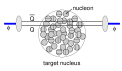
FIG. 1.: Schematic picture of color dipole propagating in nucleus which is viewed as a source of random field.

The eikonal amplitude is now factorized into the product of the transmission amplitude through each zone:

$$U_{Q\bar{Q}}({\bf d},{\bf b})=U_{n}\cdots U_{2}U_{1}\ ,$$ (24)

where the transmission amplitude for the $i$th zone, $U_{i}$, is given by the formula similar to (11):

$$U_{i}\simeq e^{i{\boldsymbol{\omega}}^{(i)}({\bf b})\cdot{\bf d}+i\theta^{(i)}({\bf b})}\ .$$ (25)

Let us introduce the matrix

$${\cal M}^{(i)}_{\alpha,\alpha^{\prime};\beta,\beta^{\prime}}({\bf d},{\bf d}^{\prime})=\overline{\langle\alpha|U_{i}({\bf d})|\beta\rangle\langle\beta^{\prime}|U_{i}^{\dagger}({\bf d}^{\prime})|\alpha^{\prime}\rangle}\ ,$$ (26)

where the average over the random field in the $i$th zone is implied by the overline. Then the survival probability of the color singlet state $|\varphi_{0}\rangle$ after penetrating through $n$ zones of uncorrelated random color fields is given by

$$S_{\varphi_{0}}(n) = \overline{|\langle\varphi_{0}|U_{Q\bar{Q}}|\varphi_{0}\rangle|^{2}}$$ (27)

$$= \int d{\bf d}d{\bf d}^{\prime}\rho_{0}({\bf d})\rho_{0}({\bf d}^{\prime})K_{0,0}({\bf d},{\bf d}^{\prime};n)\ ,$$ (28)

where $\rho_{0}({\bf d})=\int dz|\varphi_{0}({\bf d},z)|^{2}$ is the probability distribution of the color singlet dipole of size ${\bf d}$ in the wavefunction $\varphi_{0}({\bf d},z)$ and the kernel of integration is expressed in term of $\cal M$ as

$$K_{0,0}({\bf d},{\bf d}^{\prime};n)$$ (29)

$$= \overline{\langle 0|U_{Q\bar{Q}}({\bf d},n)|0\rangle\langle 0|U_{Q\bar{Q}}^{\dagger}({\bf d}^{\prime},n)|0\rangle}$$ (30)

$$= \sum{\cal M}_{0,0;\alpha_{n-1},\alpha_{n-1}^{\prime}}^{(n)}\cdots{\cal M}_{\alpha_{2},\alpha_{2}^{\prime};\alpha_{1},\alpha_{1}^{\prime}}^{(2)}{\cal M}_{\alpha_{1},\alpha_{1}^{\prime};0,0}^{(1)}\ ,$$ (31)

where the sum is taken over all intermediate color states ($\alpha_{i},\alpha_{i}^{\prime}=0,1,2,3$) . The formula (27) is non-abelian extension of the formula (7) for the positronium penetration probability. It still remains to compute the kernel function $K_{0,0}({\bf d},{\bf d}^{\prime};n)$.

For a sufficiently small zone the matrix ${\cal M}_{i}$ may be evaluated by the perturbation theory by expanding

$$U_{i}({\bf b},{\bf d}) = 1+i{\boldsymbol{\omega}}^{(i)}({\bf b})\cdot{\bf d}+i\theta^{(i)}({\bf b})$$

$$-\frac{1}{2}\left({\boldsymbol{\omega}}^{(i)}({\bf b})\cdot{\bf d}+\theta^{(i)}({\bf b})\right)^{2}+\cdots\ .$$

Calculation of the matrix elements of ${\cal M}_{i}$ requires the color average of the matrix elements of the products of $\boldsymbol{\omega}^{(i)}$ and $\theta^{(i)}$ in addition to (22) (with $L$ replaced by $l$). Since there is no preferred color direction and fields in the different zones are uncorrelated, we have

$$\overline{\langle a|\boldsymbol{\omega}^{(i)}|b\rangle\langle b^{\prime}|\theta^{(j)}|a^{\prime}\rangle}=0$$ (32)

while

$$\overline{\langle a|\theta^{(i)}|b\rangle\langle b^{\prime}|\theta^{(j)}|a^{\prime}\rangle}=\epsilon_{abc}\epsilon_{a^{\prime}b^{\prime}c}\delta_{ij}\eta({\bf b})l\ ,$$ (33)

where $\eta$ is a constant with the dimension of [length]^-1 which is also related to the transverse correlation length of the gauge fields as $\gamma_{0}$ and $\eta\sim g^{2}\Lambda_{QCD}$, $l$ is the thickness of each zone. We also need

$$\overline{\langle a|\boldsymbol{\omega}^{(i)}\cdot\boldsymbol{\omega}^{(j)}|b\rangle} = \delta_{ab}\delta_{ij}\gamma_{0}l\ ,$$ (34)

$$\overline{\langle a|\theta^{(i)}\theta^{(j)}|b\rangle} = \delta_{ab}\delta_{ij}\eta l$$ (35)

to compute all matrix elements of the $16\times 16$ matrix ${\cal M}({\bf d},{\bf d}^{\prime})$ to the order $g^{2}$.

Due to the superselection rules encoded in (22), (32), (33) and (34), the matrix ${\cal M}({\bf d},{\bf d}^{\prime})$ becomes block diagonal when it is expressed in the bases of the eigenstates of the total isospin and its $z$ components. Hereafter we adopt this new representation where Greek letters $\alpha$, $\beta$, $\dots$, stand for $(T,T_{z})=(0,0),(1,1),(1,0),(1,-1)$. In particular, the block matrix for $\alpha=\alpha^{\prime}$ and $\beta=\beta^{\prime}$:

$$M_{\alpha,\beta}({\bf d},{\bf d}^{\prime})={\cal M}^{(i)}_{\alpha,\alpha;\beta,\beta}({\bf d},{\bf d}^{\prime})$$ (36)

is given explicitly by

$$M({\bf d},{\bf d}^{\prime})=\left(\begin{array}[]{cccc}1-3r&r^{\prime}&r^{\prime}&r^{\prime}\\ r^{\prime}&1-r-s&s&0\\ r^{\prime}&s&1-r-2s&s\\ r^{\prime}&0&s&1-r-s\end{array}\right)$$ (41)

with $r=\frac{1}{2}\gamma_{0}l({\bf d}^{2}+{{\bf d}^{\prime}}^{2})$, $r^{\prime}=\gamma_{0}l{\bf d}\cdot{\bf d}^{\prime}$ and $s=\eta({\bf b})l$ where each column from top to bottom and each row from left to right now corresponds to the isospin states, $(0,0),(1,1),(1,0),(1,-1)$, respectively. All matrix elements with $\alpha=\alpha^{\prime}$ and $\beta\neq\beta^{\prime}$ which couple the block matrix $M_{\alpha,\beta}({\bf d},{\bf d}^{\prime})$ to the other components of the matrix ${\cal M}^{(i)}$ vanish by the superselection rules and $\delta_{\alpha\beta}\delta_{\alpha^{\prime}\beta^{\prime}}=0$. We can express $K_{0,0}({\bf d},{\bf d}^{\prime};n)$ in terms of the the eigenvalues $\lambda_{i}$ and the corresponding (normalized) eigenvectors ${\bf v}^{(i)}$ of the matrix $M({\bf d},{\bf d}^{\prime})$ as:

$$K_{0,0}({\bf d},{\bf d}^{\prime};n) = \sum_{i}\lambda_{i}^{n}(v_{1}^{(i)})^{2}=\sum_{i}\lambda_{i}^{n}f_{0;i}\ ,$$ (43)

where $f_{0;i}\equiv(v_{1}^{(i)})^{2}$ is the fraction of the color singlet component in the $i$th eigenstate. We find from the expression (41) of $M({\bf d},{\bf d}^{\prime})$ only two eigenstates have non-zero mixing of color singlet components for which

$$\lambda_{1} = 1-\frac{1}{2}\left(d_{+}^{2}+d_{-}^{2}-\sqrt{d_{+}^{4}+d_{-}^{4}-d_{+}^{2}d_{-}^{2}}\right)\gamma_{0}l\ ,$$ (44)

$$\lambda_{2} = 1-\frac{1}{2}\left(d_{+}^{2}+d_{-}^{2}+\sqrt{d_{+}^{4}+d_{-}^{4}-d_{+}^{2}d_{-}^{2}}\right)\gamma_{0}l$$ (45)

and

$$f_{0;1} = \frac{1}{2}-\frac{d_{+}^{2}+d_{-}^{2}}{4\sqrt{d_{+}^{4}+d_{-}^{4}-d_{+}^{2}d_{-}^{2}}}\ ,$$ (46)

$$f_{0;2} = \frac{1}{2}+\frac{d_{+}^{2}+d_{-}^{2}}{4\sqrt{d_{+}^{4}+d_{-}^{4}-d_{+}^{2}d_{-}^{2}}}\ ,$$ (47)

where $d_{\pm}^{2}=({\bf d}\pm{\bf d}^{\prime})^{2}$. Inserting (44) and (46) into (29), we obtain

$$K_{0,0}({\bf d},{\bf d}^{\prime};n) = \frac{\lambda_{1}^{n}+\lambda_{2}^{n}}{2}-\frac{(d_{+}^{2}+d_{-}^{2})(\lambda_{1}^{n}-\lambda_{2}^{n})}{4\sqrt{d_{+}^{4}+d_{-}^{4}-d_{+}^{2}d_{-}^{2}}}\ .$$ (48)

The diagonal components of the kernel $K_{0,0}({\bf d},{\bf d};n)$ can be interpreted by the construction as the probability that a color singlet rigid dipole of size ${\bf d}$ is found as color singlet after going through $n$ uncorrelated random color zones. Similarly, at ${\bf d}={\bf d}^{\prime}$ the matrix $M({\bf d},{\bf d}^{\prime})$ reduces to a matrix $P({\bf d})=M({\bf d},{\bf d})$ whose matrix element $P_{\alpha,\beta}({\bf d})=|\langle\alpha|U_{i}|\beta\rangle|^{2}$, can be interpreted as the probability of the dipole of the initial color state $\alpha$ being found in the color state $\beta$ in the final state after going through the $i$th random field zone. Since $P$ is a symmetric stochastic matrix $P=(p_{\alpha\beta})$ with $\sum_{\alpha}p_{\alpha\beta}=\sum_{\beta}p_{\alpha\beta}=1$, it has an eigenvalue of 1 for the eigenvector ${\bf v}=(1,1,1,1)^{T}$ and other eigenvalues are smaller than 1. Moreover, the matrix $P^{n}$ will approach with increasing $n$ to the matrix with all elements equal to $1/4$. This latter property implies that the transition probability from the initial isospin (color) singlet state to all color states are equal; namely, there is equi-partitioning of all different isospin states in the final state. The physical reason for the appearance of the stochastic color equi-partitioning is the cancellation of all interference terms due to the random color averaging.

The approach to the color equilibrium can be calculated explicitly from (48) as

$$K_{0,0}({\bf d},{\bf d};n) = \frac{1}{4}1^{n}+\frac{3}{4}(1-4r)^{n}=\frac{1}{4}+\frac{3}{4}e^{-n\kappa}$$ (49)

where $\kappa=-\ln(1-4r({\bf d},{\bf d}))\simeq 4r=4\gamma_{0}l{\bf d}^{2}$.

This stochastic behavior of the motion in the internal color space was already noticed in [20, 24]. It resembles to the exponential decay if one ignores the asymptotic value $1/4$ ($1/9$ in the case of SU(3)). This is not the entire story, however: the relaxation process in the color space is limited by the finite number of color degrees of freedom and the bound state survival probability still attenuates by the $1/L$ law due to the other continuous degrees of freedom, namely the transverse size ${\bf d}$ of the color dipole which is frozen during the collision, as we shall show now.

The survival probability of the bound state can be obtained by inserting (48) into (27) and performing the integral over ${\bf d}$ and ${\bf d}^{\prime}$. It is important here to take into account the interferences of the transmission amplitudes at different dipole size ${\bf d}\neq{\bf d}^{\prime}$ as we have seen in the calculation of the positronium penetration probability: the information about the internal momentum transfer ${\bf q}$ by the scattering in the random field is contained in the dependence on ${\bf d}-{\bf d}^{\prime}$ of the kernel $K_{0,0}({\bf d},{\bf d}^{\prime};n)$, namely in its off-diagonal components,

We first check that our formula contains the thin target result by setting $n=1$:

$$S_{\varphi_{0}}(1) = \int d{\bf d}d{\bf d}^{\prime}\rho_{0}({\bf d})\rho_{0}({\bf d}^{\prime})\left[1-\frac{3}{4}(d_{+}^{2}+d_{-}^{2})\gamma_{0}l\right]$$ (50)

$$= 1-3\langle{\bf d}^{2}\rangle\gamma_{0}L=1-L/L_{\rm abs}\ .$$ (51)

where we have used $L=l$ and $L_{\rm abs}=1/3\langle{\bf d}^{2}\rangle\gamma_{0}$ may be interpreted as the absorption length of the bound state. This is exactly what we have obtained already.

For thick targets with large $n$, the terms with the largest eigenvalue, $\lambda_{1}$, dominate so that

$$S_{\varphi_{0}}(n) \simeq \int d{\bf d}d{\bf d}^{\prime}\rho_{0}({\bf d})\rho_{0}({\bf d}^{\prime})$$ (53)

$$\quad\times\left[\frac{1}{2}-\frac{(d_{+}^{2}+d_{-}^{2})}{4\sqrt{d_{+}^{4}+d_{-}^{4}-d_{+}^{2}d_{-}^{2}}}\right]\lambda_{1}^{n}\ .$$

To estimate the remaining integrals we observe that the integrand is symmetric by the interchange $d_{+}\leftrightarrow d_{-}$, or equivalently by ${\bf d}^{\prime}\leftrightarrow-{\bf d}^{\prime}$, and the factor

$$\lambda_{1}^{n}=e^{n\ln\lambda_{1}}\simeq e^{-\frac{1}{2}\left(d_{+}^{2}+d_{-}^{2}-\sqrt{d_{+}^{4}+d_{-}^{4}-d_{+}^{2}d_{-}^{2}}\right)\gamma_{0}nl}$$ (54)

becomes 1 when ${\bf d}=\pm{\bf d}^{\prime}$ but decreases very rapidly as ${\bf d}\pm{\bf d}^{\prime}$ increases. Expanding the exponent in terms of $d_{-}^{2}=({\bf d}-{\bf d}^{\prime})^{2}$ and setting ${\bf d}={\bf d}^{\prime}$ in the prefactor, we may estimate roughly as

$$S_{\varphi_{0}}(n)\simeq 2\int d{\bf d}d{\bf d}^{\prime}\rho_{0}^{2}({\bf d})\frac{1}{4}e^{-\frac{3}{4}({\bf d}-{\bf d}^{\prime})^{2}\gamma_{0}L}=\frac{L_{0}}{L}\ ,$$ (55)

where the constant $L_{0}$ is given by

$$L_{0}=2\times\frac{1}{4}\times 2\times\Delta\langle{\bf d}^{2}\rangle L_{\rm abs}$$ (56)

with $\Delta=2\pi\int d{\bf d}\rho_{0}^{2}({\bf d})$ and we have used $3\langle{\bf d}^{2}\rangle\gamma_{0}=\sigma n_{0}$. This behavior is essentially the same as we have seen in the positronium case, (9), except for the factors $2\times\frac{1}{4}\times 2$: the first factor 2 arises from the symmetry by $d_{+}\leftrightarrow d_{-}$ which is specific to the case of SU(2) color charge; the second factor $\frac{1}{4}$ originates from the equi-partitioning in the color degrees of freedom and will be replaced by $1/N_{c}^{2}=1/9$ for SU(3) color; finally the last factor 2 has arisen because only one of the two eigenvalues $\lambda_{1}$ and $\lambda_{2}$ contributes at large $L$. In the case of SU(2) color charge these factors cancel accidentally, while in the case of SU(3) color charge, they are replaced by $1\times\frac{1}{3^{2}}\times 2=\frac{2}{9}$.[26]

Having established the asymptotic behavior of the survival probability $S_{\varphi_{0}}(L)$ we examine how the transition from the thin target result (50) to the thick target asymptotic behavior (55) takes place using the gaussian normalized dipole size distribution: $\rho_{0}({\bf d})=\frac{1}{\pi d_{0}^{2}}e^{-{\bf d}^{2}/d_{0}^{2}}$ which may be obtained from the ground state wave function of the non-relativistic heavy quark of the reduced particle mass $\mu$ in the harmonic oscillator potential with the frequency $\omega=1/\mu d_{0}^{2}$. In this case, $\Delta\langle{\bf d}^{2}\rangle=1$ and two length scales $L_{\rm abs}$ and $L_{0}$ coincide. The survival probability $S_{\varphi_{0}}$ then becomes a function of a single dimensionless variable $x=L/L_{\rm abs}$. The numerical result is plotted in Fig. 2 and compared with the exponential decay form obtained by the exponentiation of the thin target result (50): $1-L/L_{\rm abs}\to e^{-L/L_{\rm abs}}$. It is seen that the exponential absorption formula gives an overestimate of 20 % for the suppression at $L=L_{\rm abs}$ in the case of SU(2) color charge, while this is slightly reduced in the case of SU(3) color charge as shown in Fig. 3.

In summary, we have studied the absorption of a high energy $Q\bar{Q}$ bound state passing through random color fields taking fully into account the quantum coherence of the multiple scatterings while assuming the transverse size of the dipole is frozen by the Lorentz time dilatation. It was shown that the absorption is weaker than that given by the exponential damping form commonly used in phenomenological models for nuclear absorption and is given instead by the power law inversely proportional to the thickness of the target asymptotically. Although our calculation of penetration probability of a $Q\bar{Q}$ bound state in nuclear target is not directly applicable to the quarkonium production problem in nuclear collision, our result suggests that a special caution is needed to use the naive nuclear absorption model of quarkonium suppression at high energies, especially at RHIC and LHC energies. However, it remains to be seen how the coherence effect will show up in the nuclear collisions when one includes the production mechanism of $Q\bar{Q}$ pair[14]. We are now working on the problem and the result will be reported elsewhere.

Acknowledgments: We like to thank Gordon Baym, Arthur Hebecker, Dima Kharzeev, Larry McLerran, and Raju Venugopalan for discussions at various stages of the present work. One of the authors (H.F.) thanks the hospitality of RBRC at BNL, where a part of this work was done. This work is supported in part by the Grants-in-Aid for Scientific Research of the Ministry of Education and Sciences (Monkasho) of Japan (No. 1340067).

FIG. 2.: Penetration probability of the SU(2) color singlet state as a function of the target thickness $L/L_{\rm abs}$. The exponential form (dashed curve) is shown for reference.

FIG. 3.: Penetration probability of the SU(3) color singlet state as a function of the target thickness $L/L_{\rm abs}$.

REFERENCES

[1] For review, see X.-N. Wang and B. Jacak (edt.), Quarkonium Production in High-Energy Nuclear Collisions , Proceeding of the
RHIC/INT 1998 Winter workshop, (World Scientific, 1998).
[2] T. Matsui and H. Satz, Phys. Lett. B178 (1986) 416.
[3] C. Baglin et al. (NA38), Phys. Lett. B220 (1989) 471;
ibid.B 255 (1991) 459.
[4] J. Badier et al. Z. Phys. C 20 (1983) 101.
[5] C. Gerschel and J. Hüfner, Z. Phys. C56 (1992) 71;
and the references therein.
[6] D. Kharzeev, C. Lourenço, M. Nardi, H. Satz, Z. Phys. C74 (1997) 307.
[7] M. C. Abreu et al. (NA50), Phys. Lett. B410 (1997) 337.
[8] J.-P. Blaizot and J. Y. Ollitrault, Phys. Rev. Lett. 77 (1996) 1703.
[9] H. Satz, Rep. Prog. Phys. 63 (2000) 1511.
[10] H. Feshbach, in Asymptotic Realms of Physics,
ed. A.H. Guth et al., The MIT Press (1983) pp95.
[11] J. -P. Blaizot and E. Iancu, Phys. Rev. Lett. 76 (1996) 3080.
[12] B. Z. Kopeliovich, A. Tarasov, and J. Hüfner, Nucl. Phys. A696 (2001) 669.
[13] D. Kharzeev and H. Satz, Phys. Lett. B366 (1996) 316.
[14] P. Hoyer and S. Peigné, Phys. Rev. D 59 (1999) 034011.
[15] L.L. Nemenov, Sov. J. Nucl. Phys. 34 (1981) 726; and
the references therein.
[16] V.L. Lyuboshitz and M.I. Podgoretskiĭ, JETP 54 (1981) 827.
[17] Al.B. Zamolodchikov, B.Z. Kopoliovich and L.I. Lapidus,
JETP Lett. 33(1981) 595.
[18]J. Hüfner, B. Povh and S. Gardner, Phys. Lett.B238
(1990) 103.
[19] G. Baym, Adv. Nucl. Phys. 22 (1996) 101; and the references therein.
[20] J. Hüfner, C.H. Lewenkopf and M.C. Nemes,
Nucl. Phys. A518 (1990) 297.
[21] G. Bertsch, S. J. Brodsky, A. S. Goldhaber, and J. G. Gunion,
Phys. Rev. Lett. 47 (1981) 297.
[22] S. J. Brodsky and A. H. Mueller, Phys. Lett. B206 (1988) 685.
[23] A. H. Mueller, hep-ph/0111244 (Lectures at the 2001 Cargése Summer School).
[24] A. Hebecker and H. Weigert, Phys. Lett.B432 (1998) 15.
[25] L. McLerran and R. Venugopalan, Phys. Rev. D 49 (1994) 2233.