Strange Disoriented Chiral Condensate

Abstract

Disoriented chiral condensate can produce novel fluctuations of kaons as well as pions. Robust statistical observables can be used to extract the novel fluctuations from background contributions in $K_{S}^{0}K^{\pm}$ measurements in nuclear collisions. To illustrate how this can be done, I present new event-generator computations of these observables.

I Introduction

Relativistic nuclear collisions can produce matter in which chiral symmetry is restored. One possible consequence of the restoration and the subsequent re-breaking of chiral symmetry is the formation of disoriented chiral condensates (DCC) – transient regions in which the average chiral order parameter differs from its value in the surrounding vacuum DCCreview ; qmrev1 ; qmrev2 . Previous efforts to describe DCC signals have focused on pion production.

In Ref. GavinKapusta , Kapusta and I have explored the possible influence of DCC on kaon production, inspired by the explanation due to Kapusta and Wong KapustaWong of measurements of $\Omega$ and $\overline{\Omega}$ baryon enhancement SPSbaryons at $17$ $A$ GeV at the CERN SPS in terms of the production of many small DCC regions within individual collision events. If true, Ref. KapustaWong implies that the evolution of the condensate can have a significant effect on strange particle production. The importance of strange degrees of freedom in describing chiral restoration has been long appreciated PisarskiWilczek ; Columbia ; GGP2 ; Karsch ; Lenaghan , but simulations of the three flavor linear sigma model had suggested that strange kaon fields are much less important than the pion fields Randrup . Nevertheless, the $\Omega$ and $\overline{\Omega}$ data demand that we explore without prejudice techniques for measuring kaon fluctuations.

A further implication of Ref. KapustaWong is that the DCC regions must be rather small, with a size of about $2$ fm. Such a size is consistent with predictions based on dynamical simulations of the two flavor linear sigma model GGP1 . More importantly, the DCC search for anomalous event structure in neutral and charged pions by the WA98 Collaboration at the SPS has revealed no evidence of large DCC ”domains” qmrev2 . Note that I loosely use the word ”domain” to refer to spatial regions in which the condensate is somehow coherent. I stress that no thermodynamically stable domain structures are expected in theoretical descriptions of DCC.

In this paper I study kaon isospin fluctuations in the presence of many small DCC. In the next section I discuss how DCC may lead to kaon fluctuations. Following Ref. GavinKapusta , I compute the probability distribution that describe the DCC contribution to these fluctuations and combine the DCC fluctuations with a contribution from a random thermal background. Pion fluctuations due to many small DCC have been addressed by Amado and Lu AmadoLu and Chow and Cohen ChowCohen . Here we focus on kaon fluctuations; pion as well as kaon results are presented in Ref. GavinKapusta . In sec. 4 I assess robust statistical observables that can be used to measure the impact of many small DCC at RHIC and LHC. In sec. 5 I present work in progress on event generator simulations to understand the magnitude and centrality dependence of the statistical observables in the absence of DCC. In particular, I obtain a dynamic isospin fluctuation observable analogous to the dynamic charge observable used to measure net charge fluctuations at RHIC Voloshin . Of the quantities considered, this observable isolates the DCC effect from other sources of fluctuations best.

II Strange DCC

To illustrate how a strange DCC can form, let us first consider QCD with only up and down quark flavors. Equilibrium high temperature QCD respects chiral symmetry if the quarks are taken to be massless. This symmetry is broken below $T_{c}\sim 150$ MeV by the formation of a chiral condensate $\langle\sigma\rangle\sim\langle\overline{u}u+\overline{d}d\rangle$ that is a scalar isopin singlet. However, chiral symmetry implies that $\sigma$ is degenerate with a pseudoscalar isospin triplet of fields with the same quantum numbers as the pions. In reality, chiral symmetry is only approximate and the 140 MeV pion mass is different from the $800\pm 400$ MeV mass of the leading sigma candidate pdg . Nevertheless, lattice calculations exhibit a dramatic drop of $\langle\sigma\rangle$ near $T_{c}$ at finite quark masses.

A DCC can form when a heavy ion collision produces a high energy density quark-gluon system that then rapidly expands and cools through the critical temperature. Such a system can initially break chiral symmetry along one of the pion directions, but must then evolve to the $T=0$ vacuum by radiating pions. A single coherent DCC radiates a fraction $f_{\pi}$ of neutral pions compared to the total that satisfies the probability distribution

$$\rho_{1}(f_{\pi})={{1}\over{2f_{\pi}^{1/2}}}\,\,\,\,\,\,\,\,\,\,\,\,\,\,\,\,0<f_{\pi}\leq 1,$$ (1)

Anselm ; Blaizot ; Bjorken . Such isospin fluctuations constitute the primary signal for DCC formation in the pion sector. The enhancement of baryon-antibaryon pair production is a secondary effect due to the relation between baryon number and the topology of the pion condensate field KapustaSrivastava .

This two flavor idealization only applies if the strange quark mass $m_{s}$ can be taken to be infinite. Alternatively, if I take $m_{s}=m_{u}=m_{d}=0$, then the chiral condensate would be an up-down-strange symmetric scalar field. The more realistic case of $m_{s}\sim 100$ MeV is between these extremes, so that $\langle\sigma\rangle\sim\langle\cos\theta(\overline{u}u+\overline{d}d)+\sin\theta(\overline{s}s)\rangle$. The mixing angle $\theta$ is highly uncertain since it depends on the sigma mass together with the $\pi,K,\eta$ and $\eta^{\prime}$ masses and the $\eta-\eta^{\prime}$ mixing angle GGP2 . A disoriented condensate can evolve by radiating $\pi,K,\eta$ and $\eta^{\prime}$ mesons, with the neutral pion fraction satisfying (1). Randrup and Schäffner-Bielich find that the kaon fluctuations from a single large DCC satisfy Randrup

$$\rho_{1}(f_{K})=1\,\,\,\,\,\,\,\,\,\,\,\,\,\,\,\,0\leq f_{K}\leq 1,$$ (2)

where $f_{K}=(K^{0}+\overline{K}^{0})/(K^{+}+K^{-}+K^{0}+\overline{K}^{0})$. Moreover, the condensate fluctuations can now produce strange baryon pairs KapustaWong . Linear sigma model simulations indicate that pion fluctuations dominate three-flavor DCC behavior, while the fraction of energy imparted to kaon fluctuations is very small due to the kaons’ larger mass. On the other hand, domain formation may be induced by other mechanisms such as kaon condensation at high baryon density Kaplan , bubble formation qm95 or decay of the Polyakov loop condensate Pisarski .

III DCC Mesons from Many Small Domains

Why does the DCC’s size matter? Pion measurements in individual collision events can distinguish DCC isospin fluctuations from a thermal background only if the disoriented region is sufficiently large qmrev1 . DCC can then be the dominant source of pions at low transverse momenta, since $\langle p_{t}\rangle\sim 1/R$ for a coherent region of size $R$. Experiments focusing on low $p_{t}$ can study neutral and charged pion fluctuations Bjorken , wavelet Ina and HBT signals qmrev1 ; HBT to extract detailed information. In contrast, for small domains ($R<3$ fm qmrev1 ) DCC signals are hidden by fluctuations due to ordinary incoherent production mechanisms. This holds even if many such regions are produced per event. DCC mesons from small regions may have momenta of a few hundred MeV, nearer the $pp$ mean value. Different regions would not add coherently to alter HBT, nor would their small spatial structures affect wavelet analysis.

Importantly, baryon pair enhancement KapustaWong is substantial only if there are many small incoherent regions. The large winding numbers that produce baryon-antibaryon pairs require many small regions with random relative orientations of the pion field. To describe strange antibaryon enhancement, Kapusta and Wong assume roughly 100 DCC regions of size roughly $2$ fm KapustaWong . Topological models of baryon-antibaryon pair production successfully describe $e+e-$ and hadronic collision data EllisKowalski . The connection of DCC to topological pair production was pointed out in Ref. KapustaSrivastava ; see also DeGrand .

To compute the distribution of kaons due to many small DCC regions, define $f=(K^{0}+\overline{K}^{0})/(K^{+}+K^{-}+K^{0}+\overline{K}^{0})$. To an excellent approximation the number of neutral kaons is equal to twice the number of short-lived neutral kaons $K_{S}$ which are more readily measurable in high energy heavy ion collisions. The fraction $f$ ranges from 0 to 1. The statistical distribution in $f$ for a single domain is $\rho_{1}(f)=1$. The distribution for $n$ randomly oriented, independent domains is

$$\rho_{n}(f)=\int\prod_{k=1}^{n}df_{k}\,\rho_{1}(f_{k})\,\delta\left(f-\frac{1}{n}\sum_{j=1}^{n}f_{j}\right)\,.$$ (3)

In GavinKapusta I obtain

$$\rho_{n}(f)=n^{2}\sum_{0\leq k<n(1-f)}(-1)^{k}\frac{[n(1-f)-k]^{n-1}}{k!(n-k)!}\,.$$ (4)

In the limit that $n\gg 1$, this distribution tends toward a Gaussian of mean $\langle f\rangle=1/2$ and standard deviation $\sigma=\{12n\}^{-1/2}$. Results for pions are presented in GavinKapusta .

In a more realistic scenario some kaons will come from the decay or realignment of DCC domains and some will come from more conventional sources. I shall refer to the latter as random or thermal, even though that may be a bit of a misnomer. What I mean by random or thermal is that the distribution of kaons from non-DCC sources is

$$\rho_{0}(f_{0})=\frac{1}{2\pi\sigma_{0}^{2}}\exp\left[-(f_{0}-1/2)^{2}/2\sigma_{0}^{2}\right]\,.$$ (5)

For a completely random source the width $\sigma_{0}$ is related to the total number $N_{\rm random}$ of non-DCC kaons by

$$\sigma^{2}_{0}=\frac{1/2(1-1/2)}{N_{\rm random}}=\frac{1}{4N_{\rm random}}\,.$$ (6)

Now let us assume that a fraction $\alpha_{K}$ of all kaons come from non-DCC sources and the remaining fraction $\beta_{K}=1-\alpha_{K}$ come from $n\gg 1$ independent DCC domains. Letting $N$ denote the total number of kaons, I have $N_{\rm random}=\alpha_{K}N$ and $N_{\rm DCC}=\beta_{K}N$. Folding together two Gaussians gives a Gaussian.

$$\rho_{K}(f) = \int df_{0}df_{n}\rho_{0}(f_{0})\rho_{n}(f_{n})\delta(f-\alpha_{K}f_{0}-\beta_{K}f_{n})$$ (7)

$$= \frac{1}{\sqrt{2\pi\Delta_{K}^{2}}}\exp\left[-(f-1/2)^{2}/2\Delta_{K}^{2}\right]$$

For a thermal source plus $n$ DCC domains, the net width is

$$\Delta_{K}^{2}=\frac{\alpha_{K}}{4N}+\frac{\beta_{K}^{2}}{12n}=\frac{1}{4N}+\left\{\frac{\beta_{K}^{2}}{12n}-\frac{\beta_{K}}{4N}\right\}\,.$$ (8)

The expression in curly brackets at the end represents the difference between the actual width and the width the distribution would have if there was no contribution from DCC kaons. This change in the width may be positive or negative, depending on the parameters.

IV Statistical Analysis

Detection of small incoherent DCC regions in high energy heavy ion collisions requires a statistical analysis in the $\pi^{0}\pi^{\pm}$ or the $K_{S}^{0}K^{\pm}$ channels. Neutral mesons can be detected by the decays $\pi^{0}\rightarrow\gamma\gamma$ or $K^{0}_{S}\rightarrow\pi^{+}\pi^{-}$. The analysis we propose in GavinKapusta is sensitive to correlations due to isospin fluctuations. We expect these correlations to vary when DCC regions increase in abundance or size as centrality, ion-mass number $A$, or beam energy are changed. Correlation results combined with other signals, such as baryon enhancement KapustaWong , can be used to build a circumstantial case for DCC production.

Correlations of $\pi^{0}\pi^{\pm}$ and $K_{S}^{0}K^{\pm}$ can be determined by measuring the robust isospin covariance,

$$R_{c0}={{\langle N_{c}N_{0}\rangle-\langle N_{c}\rangle\langle N_{0}\rangle}\over{\langle N_{c}\rangle\langle N_{0}\rangle}},$$ (9)

where $N_{0}$ and $N_{c}$ are the number of neutral and charged mesons. I take $N_{0}=N_{\pi^{0}}$ and $N_{c}=N_{\pi^{+}}+N_{\pi^{-}}$ for pion fluctuations and $N_{0}=2N_{K^{0}_{S}}$ and $N_{c}=N_{K^{+}}+N_{K^{-}}$ for kaon fluctuations. The ratio (9) has two features that are convenient for experimental determination. First, this observable is independent of detection efficiency as are the “robust” ratios discussed in Taylor . Robust observables are useful for DCC studies because charged and neutral particles are identified using very different techniques and, consequently, are detected with different efficiency. Observe that robust quantities are not affected by the unobserved $K_{L}^{0}$, since the strong-interaction eigenstates $K^{0}$ and ${\overline{K}}^{0}$ are a superposition $K_{L}^{0}$ and $K_{S}^{0}$ until their decay well outside the collision region. Second, since (9) is obtained from a statistical analysis, individual $\pi^{0}\rightarrow\gamma\gamma$ or $K^{0}_{S}\rightarrow\pi^{+}\pi^{-}$ need not be fully reconstructed in each event. This feature is crucial because it would be extraordinarily difficult – if not impossible – to reconstruct a low momentum $\pi^{0}$ in heavy ion collisions except on a statistical basis.

Next I define robust variance

$$R_{aa}={{\langle N_{a}^{2}\rangle-\langle N_{a}\rangle^{2}-\langle N_{a}\rangle}\over{\langle N_{a}\rangle^{2}}},$$ (10)

where $a=c$ or 0. To see why (10) is robust, denote the probability of detecting each meson $\epsilon$ and the probability of missing it $1-\epsilon$. For a binomial distribution the average number of measured particles is $\langle N_{a}\rangle^{\rm exp}=\epsilon\langle N_{a}\rangle$ while the average square is $\langle N_{a}^{2}\rangle^{\rm exp}=\epsilon^{2}\langle N_{a}^{2}\rangle+\epsilon(1-\epsilon)\langle N_{a}\rangle$. I then find

$$R_{aa}^{\rm exp}=R_{aa},$$ (11)

independent of $\epsilon$ Pruneau ; the proof that (9) is robust is similar. The ratios (9) and (10) are strictly robust only if the efficiency $\epsilon$ is independent of multiplicity. Further properties and advantages of these and similar quantities are discussed in Pruneau .

To study DCC fluctuations I define the dynamic isospin observable

$$\nu_{\rm dyn}^{c0}=R_{cc}+R_{00}-2R_{c0}.$$ (12)

Analogous observables have been employed to study net charge fluctuations in particle physics Whitmore ; Boggild and were considered in a heavy ion context in Voloshin and Mrowczynski . This quantity can be written in terms of

$$\nu^{c0}=\left\langle\left({{N_{0}}\over{\langle N_{0}\rangle}}-{{N_{c}}\over{\langle N_{c}\rangle}}\right)^{2}\right\rangle.$$ (13)

To isolate the dynamical isospin fluctuations from other sources of fluctuations, one obtains (12) by subtracting from (13) the uncorrelated Poisson limit $\nu_{\rm stat}^{c0}=\langle N_{0}\rangle^{-1}+\langle N_{c}\rangle^{-1}$. Indeed, we show in (19) below that the quantity (12) depends primarily on the fluctuations of the neutral fraction $f$, while the individual ratios (9) and (10) have additional contributions.

I illustrate the effect of DCC on the dynamic isospin fluctuations by writing $N_{0}=fN$ and $N_{c}=(1-f)N$. Small fluctuations on $f$ or $N$ results in the changes

$$\frac{\Delta N_{0}}{\langle N_{0}\rangle}={{\Delta N}\over{\langle N\rangle}}+{{\Delta f}\over{\langle f\rangle}},\,\,\,\,\,\,\,\,\,\,\,\,\,\,\,\,\,\,\frac{\Delta N_{c}}{\langle N_{c}\rangle}={{\Delta N}\over{\langle N\rangle}}-{{\Delta f}\over{1-\langle f\rangle}}\,.$$ (14)

I obtain the average

$${{\langle\Delta N_{0}^{2}\rangle}\over{\langle N_{0}\rangle^{2}}}=v+{{2c}\over{\langle N\rangle\langle f\rangle}}+{{\Delta^{2}}\over{\langle f\rangle^{2}}}.$$ (15)

Here the contribution of the variance of the total number of mesons is $v\equiv\langle\Delta N^{2}\rangle/\langle N\rangle^{2}$ and the charge-total covariance is $c\equiv\langle\Delta N\Delta f\rangle$. DCC formation primarily effects the charge fluctuation contribution, $\Delta^{2}\equiv\langle(\Delta f)^{2}\rangle$, from (15) or (17). Similarly,

$${{\langle\Delta N_{c}^{2}\rangle}\over{\langle N_{c}\rangle^{2}}}=v-{{2c}\over{\langle N\rangle(1-\langle f\rangle)}}+{{\Delta^{2}}\over{(1-\langle f\rangle)^{2}}}\,,$$ (16)

and

$$R_{c0}=v+\left({{1}\over{\langle f\rangle}}-{{1}\over{1-\langle f\rangle}}\right){{c}\over{\langle N\rangle}}-{{\Delta^{2}}\over{(1-\langle f\rangle)^{2}}}\,$$ (17)

where $R_{c0}$ is given by (9). Using (21) I get

$$\nu_{\rm dyn}^{c0}={{1}\over{\langle f\rangle(1-\langle f\rangle)}}\left({{\Delta^{2}}\over{\langle f\rangle(1-\langle f\rangle})}-{{1}\over{\langle N\rangle}}\right).$$ (18)

This observable isolates the isospin fluctuations, whereas the individual $R_{ab}$ depend on the fluctuations in total meson number, $v$ and $c$ as well.

I estimate the effect of DCC on the dynamical fluctuations (18) using (6) and (8). I take $\langle N\rangle=N_{K}$ for kaons and $\langle N\rangle=N_{\pi}$ for pions; these are the total number of mesons of the indicated kind. For kaons

$$\nu_{\rm dyn}^{c0}({\rm K~{}DCC})=4\beta_{K}\left(\frac{\beta_{K}}{3n}-\frac{1}{N_{K}}\right)\,.$$ (19)

These quantities can be positive or negative depending on the magnitude of $\beta$ compared to the number of domains per kaon. In fact the dynamical fluctuation may even be positive for one kind of meson and negative for the other.

V Fluctuations in the Absence of DCC

Let us now discuss work in progress in which Abdel-Aziz and I use event generators to simulate conventional sources of kaon fluctuations hamlet . In the absence of DCC, $\alpha=1$ and $\beta=0$ so that (19) implies $\nu_{\rm dyn}^{c0}\equiv 0$. On the other hand, incomplete equilibration may result in dynamical correlations in nuclear collisions not described by (5). Little is known from $pp$ experiments about kaon fluctuations. Event generators such as HIJING and URQMD models both yield negative values of $\nu_{\rm dyn}^{c0}$ in pp collisions. HIJING simulations of central Au+Au at 200 $A$ GeV in the rapidity range $-0.5<y<0.5$ yield $\nu_{\rm dyn}^{c0}\approx-0.002$ for 47 $K^{+}$ and 44 $K_{S}^{0}$ on average HIJING .

The onset of DCC formation can substantially change the value of $\nu_{\rm dyn}^{c0}$. To search for this onset it is useful to study fluctuations as a function of collision centrality. I use HIJING to estimate the influence of conventional collision geometry and dynamics on the centrality dependence. However, I find that one can understand the HIJING results quite simply using the wounded nucleon model. In a multiple collision models such as the wounded nucleon model, one describes a nucleus-nucleus collision as a superposition of M independent nucleon-nucleon sub-collisions. The robust variance and covariance satisfy

$$R_{ab}={{r_{ab}}\over{\langle M\rangle}}+{{\langle M^{2}\rangle-\langle M\rangle^{2}}\over{\langle M\rangle^{2}}}\,,$$ (20)

where the $r_{ab}$ are coefficients describing the fluctuations in each sub-collision and $a,b$ can equal either $c$ or $0$. The dynamical isospin observable,

$$\nu_{\rm dyn}^{c0}=R_{cc}+R_{00}-2R_{c0}={{\nu_{0}}\over{\langle M\rangle}},$$ (21)

is independent of the contribution from the fluctuations of $M$. In the wounded nucleon model, $M$ is given at each impact parameter by the number of participant nucleons.

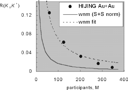
Figure 1: Scaled covariance for HIJING compared to the wounded nucleon model normalized to HIJING S+S (solid curve) and fit (dashed).

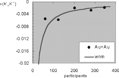
Figure 2: Dynamic isospin observable for the same simulated collisions. Wounded nucleon result agrees with HIJING S+S normalization.

In figs. 1 and 2, I show the kaon covariance (9) and dynamical isospin observable (12) as functions of the number of participants $M$ computed from 50,000 HIJING events for Au+Au at 200 A$GeV$ in the rapidity range $-0.5<y<0.5$ compared to wounded nucleon model calculations (20). The number of participants at impact parameter $b$ for a symmetric Au+Au collision is computed using $M(b)=2\int dsT(s)\{1-e^{-\sigma_{NN}T(b-s)}\}$, where $T(b)=\int\rho(z,b)dz$ is the familiar nuclear thickness function and $\rho$ is the three-parameter Fermi nuclear density for Au. In fig. 1, the solid curve is determined using (20) with a coefficient $r_{c0}$ computed from 50,000 S+S collisions, while the dashed curve is obtained by varying $r_{c0}$ to fit Au+Au. The HIJING results scale roughly as $R_{c0}\propto M^{-1}$ as expected, but the difference from the wounded nucleon model are rather large.

Figure 2 shows the dynamical isospin observable as a function of $M$ from HIJING. The solid curve is obtained from (21) with $\nu_{0}$ determined from HIJING S+S. I find that the wounded nucleon model is in excellent agreement with HIJING, suggesting that the correlations that increase $R_{ab}$ compared to the wounded nucleon model are similar for all kaon charge states. The agreement of HIJING and the wounded nucleon model in fig. 2 is likely due to the following. First, baryon stopping is unimportant at the high RHIC energy. Different numbers of protons and neutrons would alter the isospin balance. Second, high $p_{T}$ aside, the way HIJING describes soft interactions is quite similar to the wounded nucleon model, since it doesn’t incorporate final state cascading. To understand the effect of cascading, we are currently studying URQMD collisions hamlet .

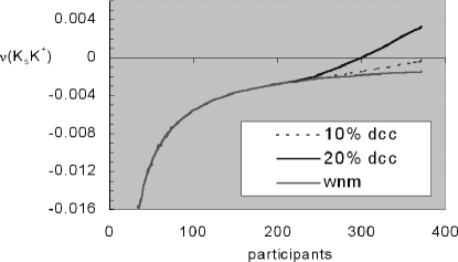
Figure 3: Scaled kaon covariance vs. number of participants as above plus a contribution from 10 DCC domains.

To illustrate the possible scenario for the onset of DCC effects, I assume that DCC kaons add to the kaons from multiple sub-collisions according to

$$\nu_{\rm dyn}^{c0}=\beta^{2}\nu_{dcc}+(1-\beta^{2})\nu_{wnm},$$ (22)

where $\beta$ is the fraction of DCC kaons, $\nu_{dcc}$ is the DCC contribution given by (10) and $\nu_{wnm}$ is given by (21). I assume that DCC production above an impact parameter $b_{0}$ exhibits a threshold behavior, $\beta=\beta_{0}[1-(b/b_{0})^{2}]$, where $b_{0}$ and $\beta_{0}$ are ad hoc constants. In fig. 4, I show estimates assuming that 10 domains contribute kaons in the range $-0.5<y<0.5$ for $b_{0}\sim 6$ fm, varying the dcc fraction $\beta_{0}$ between 10% and 20%. Note that the DCC contribution to $\nu$ is positive for these values.

VI Discussion and Conclusion

Reference KapustaWong argued that the anomalous abundance and transverse momentum distributions of $\Omega$ and $\overline{\Omega}$ baryons in central collisions between Pb nuclei at 17 $A$ GeV at the CERN SPS is evidence that they are produced as topological defects arising from the formation of many domains of disoriented chiral condensates (DCC) with an average domain size of about 2 fm. Motivated by this interpretation, Kapusta and I studied the effect of DCC on the distribution of the fractions of neutral kaons and pions in GavinKapusta .

The DCC pioneers Anselm ; Blaizot ; Bjorken ; DCCreview had hoped that a large percentage of pions might be emitted from just a few big domains, on the order of 5 to 8 fm (kaons were not considered). Such large domains have been ruled out at SPS qmrev2 , but remain possible at RHIC. More conservatively, as the number of domains grow and their average size diminishes, the impression left on the fluctuations in the neutral fraction becomes more subtle and less unique. For many small domains, statistical measurements of both neutral kaons (pions) and charged kaons (pions) are needed to observe the rather small isospin fluctuations. We have identified robust observables for that purpose. In particular, we have shown that the dynamical isospin observable (12) is sensitive to DCC but not to thermal or multiple-collision sources of fluctuations, as discussed in the text near eqs. (19) and (21) respectively. While HIJING simulations support this conclusion, more work remains. For example, one can use URQMD to study the effect of final state scattering on this observable. Isospin fluctuations can appear as changes in the magnitude of the dynamical isospin observable as centrality is varied. We emphasize that similar consequence may follow from any mechanism that produces many small domains that decay to pions and kaons, such as the Polyakov Loop Condensate Pisarski .

I am grateful to Joe Kapusta for a very enjoyable collaboration and thank M. Abdel-Aziz, R. Bellwied, C. Pruneau, S. Voloshin and, especially, H. Stöcker for many useful discussions. This work was supported in part by U.S. DOE Grant number DE-FG02-92ER40713.

References

- (1) K. Rajagopal and F. Wilczek, Nucl. Phys. B399, 395 (1993); B404, 577 (1993); K. Rajagopal, in Quark-Gluon Plasma 2, R. C. Hwa ed., (World Scientific, 1995); hep-ph/9504310.
- (2) S. Gavin, Nucl. Phys. A590, 163c (1995).
- (3) T. Nayak, et al. (WA98 Collaboration), Nucl. Phys. A638, 249c (1998); Phys. Rev. C 64 011901 (2001).
- (4) S. Gavin and J. I. Kapusta, Phys. Rev. C, to be published; nucl-th/0112083.
- (5) J. B. Kinson, J. Phys. G 25, 143 (1999).
- (6) J. I. Kapusta and S. M. Wong, Phys. Rev. Lett. 86, 4251 (2001); nucl-th/0012006.
- (7) S. Gavin, A. Gocksch and R. D. Pisarski, Phys. Rev. Lett. 72, 2143 (1994); hep-ph/9310228.
- (8) R. D. Pisarski and F. Wilczek, Phys. Rev. D 29, 338 (1984).
- (9) F. R. Brown et al., Phys. Rev. Lett. 65, 2491 (1990).
- (10) S. Gavin, A. Gocksch and R. D. Pisarski, Phys. Rev. D 49, 3079 (1994); hep-ph/9311350.
- (11) C. Schmidt, F. Karsch and E. Laermann, hep-lat/0110039.
- (12) J. T. Lenaghan, D. H. Rischke and J. Schaffner-Bielich, Phys. Rev. D 62, 085008 (2000); nucl-th/0004006.
- (13) J. Schaffner-Bielich and J. Randrup, Phys. Rev. C 59, 3329 (1999); nucl-th/9812032.
- (14) R. D. Amado and Y. Lu, Phys. Rev. D 54, 7075 (1996); hep-ph/9608242.
- (15) C. K. Chow and T. D. Cohen, Phys. Rev. C 60, 054902 (1999); nucl-th/9908013.
- (16) S. A. Voloshin [STAR Collaboration], nucl-ex/0109006.
- (17) D. E. Groom et al. [Particle Data Group Collaboration], Eur. Phys. J. C 15, 1 (2000).
- (18) A. A. Anselm and M. G. Ryskin, Phys. Lett. B266, 482 (1991).
- (19) J.-P. Blaizot and A. Kryzywicki, Phys. Rev. D 46, 246 (1992).
- (20) J. D. Bjorken, K. L. Kowalski and C. C. Taylor, Report SLAC-PUB-6109 (1993), hep-ph/9309235, unpublished.
- (21) J. I. Kapusta and A. M. Srivastava, Phys. Rev. D 52, 2977 (1995); hep-ph/9404356.
- (22) A. E. Nelson, D. B. Kaplan, Phys. Lett. B192, 193 (1987).
- (23) J. I. Kapusta, A. P. Vischer and R. Venugopalan, Phys. Rev. C 51, 901 (1995); nucl-th/9408029; J. I. Kapusta and A. P. Vischer, Z. Phys. C75, 507 (1997); nucl-th/9605023.
- (24) A. Dumitru and R. D. Pisarski, Phys. Lett. B504, 282 (2001); hep-ph/0010083.
- (25) Z. Huang, I. Sarcevic, R. Thews and X. N. Wang, Phys. Rev. D 54, 750 (1996); hep-ph/9511387.
- (26) H. Hiro-Oka and H. Minakata, Phys. Lett. B425, 129 (1998) [Erratum-ibid. B434, 461 (1998)]; hep-ph/9712476.
- (27) J. R. Ellis and H. Kowalski, Phys. Lett. B214, 161 (1988); Nucl. Phys. B327, 32 (1989).
- (28) T. A. DeGrand, Phys. Rev. D 30, 2001 (1984); J. R. Ellis, U. W. Heinz and H. Kowalski, Phys. Lett. B233, 223 (1989).
- (29) T. C. Brooks et al. [MiniMax Collaboration], Phys. Rev. D 55, 5667 (1997); hep-ph/9609375; Phys. Rev. D 61, 032003 (2000); hep-ex/9906026.
- (30) C. Pruneau, S. Gavin and S. A. Voloshin, nucl-ex/0204011.
- (31) J. Whitmore, Phys. Rep. 27, 187 (1976).
- (32) H. Boggild and T. Ferbel, Ann. Rev. Nucl. Part. Sci. 24, 451 (l974).
- (33) S. Mrowczynski, nucl-th/0112007.
- (34) X. N. Wang and M. Gyulassy, Phys. Rev. D 44, 3501 (1991); S. E. Vance and M. Gyulassy, Phys. Rev. Lett. 83, 1735 (1999); nucl-th/9901009; S. E. Vance, M. Gyulassy and X. N. Wang, Phys. Lett. B443, 45 (1998); nucl-th/9806008.
- (35) M. Abdel-Aziz and S. Gavin, in progress.