Virtual-pion and two-photon production in pp scattering

Abstract

Two-photon production in pp scattering is proposed as a means of studying virtual-pion emission. Such a process is complementary to real-pion emission in pp scattering. The virtual-pion signal is embedded in a background of double-photon bremsstrahlung. We have developed a model to describe this background process and show that in certain parts of phase space the virtual-pion signal gives significant contribution. In addition, through interference with the two-photon bremsstrahlung background, one can determine the relative phase of the virtual-pion process.

I Introduction

Near-threshold pion production in proton-proton scattering has a long history Sta58 ; Hac78 . More recently it has attracted much attention after precise data have become available from experiments at IUCF Mey92 and Bon95 . These showed that this relatively simple reaction is apparently poorly understood. Earlier works showed large discrepancy between the calculations and the data Mil91 ; Nis92 . Later several different mechanisms such as heavy meson exchange Lee93 ; Hor94 , off-shell structure of the T-matrix Her95O ; Ada97 , heavy meson exchange currents VKo96 , and approximations used in the calculation of the loop contributions Sat97 have been proposed to explain this problem in the earlier calculations. Calculations in a relativistic one-boson-exchange model Eng96 and non-relativistic potential model Han98b on the other hand appear to reproduce the data rather well.

In this work we propose to extend the available kinematical regime for neutral-pion production by investigating the process of virtual $\pi^{0}$ emission which can be observed through its two-photon decay. The interest in this process is manyfold. For example, the importance of off-shell form factors or the off-shell structure of the T-matrix Her95O ; Ada97 can be investigated when an extended kinematical regime is available for measuring this reaction. In addition, studying virtual-pion production below the threshold for real-pion production in proton-proton scattering implies an important simplification in the description of the process since the inelasticities, always present in the pion-nucleon scattering, are absent for virtual pions. More importantly, interference of two-photon production via a virtual pion with the background due to two-photon bremsstrahlung will determine the relative sign of the matrix elements. This will allow for a better insight in the underlying pion-production process. The sign is relevant regarding the discussion of the constructive v.s. destructive interference of the higher-order diagrams in a field-theoretical approach Par96 ; Coh96 ; Ged99a ; Sat97 .

To describe the “background”, two-photon bremsstrahlung, cross section we have developed a Soft-Photon Model (SPM) for two-photon emission.

In this context SPM implies a covariant model satisfying gauge invariance, which obeys the proper low-energy theorem for small photon momenta (for example, for the one-photon bremsstrahlung the leading two orders in powers of the photon energy satisfy model-independent constraints Low58 ). As a first step towards such an SPM, we develop in section II a new SPM for the single-photon bremsstrahlung amplitude. This novel SPM, based on a power-series expansion of the T-matrix, combines ideas of the two SPM’s which are frequently used for single-photon bremsstrahlung in $pp$ scattering: the original SPM Nym68 ; Fea86 , which is directly inspired by the derivation of the low-energy theorem for bremsstrahlung by Low Low58 , and a later one proposed in ref. Lio93 , which has been very successful in reproducing the observed cross sections Lio95 ; Hui99 . The important distinction of the new SPM from the existing two is that no explicit contact terms, or the so-called internal contributions, need to be introduced. This feature makes it the most suitable model for developing the Two-Soft-Photon Model (2SPM) as discussed at the end of section II. Such a 2SPM may also be used to calculate the background two-photon signal in the search for di-baryon states Khr01 .

In this work, where the emphasis is placed on the feasibility of detecting the virtual-$\pi^{0}$ signal, we have also employed a relatively simple covariant model to describe the pion-emission process. This model is discussed in detail in section III. The predictions of this model are shown to reproduce data on real-pion emission.

In section IV explicit calculations are presented for two-photon production where both mechanisms, bremsstrahlung and virtual-$\pi^{0}$ emission, are taken into account. The parts of phase space are indicated where the second mechanism is relatively large. It is also demonstrated that interference between the two processes is very important.

II The soft-photon model

A starting point in an SPM description of bremsstrahlung in $pp$ scattering is that the dominant -pole- contribution to the amplitude is derived from the Feynman diagrams where the photon is radiated off the external legs Low58 . To this leading order, several higher-order, non-pole, terms need to be added which may correspond to meson-exchange, form-factor, and rescattering contributions. The observation made by Low, which is the essence of the low-energy theorem Low58 , is that in any description for the amplitude which has the correct pole structure and is gauge invariant, in a power expansion of the amplitude, the leading two powers are model independently given by an expression involving only on-shell (i.e. measurable) quantities, such as the non-radiative NN T-matrix, charge and magnetic moment of the nucleon.

In the formulation of a SPM description for bremsstrahlung this model independence of the leading contributions to the amplitude is exploited. In principle, the T-matrix entering in each of the pole diagrams needs to be evaluated at different off-shell kinematics. In an SPM one relates the off-shell T-matrix to the T-matrix at an appropriately chosen on-shell kinematical point. Based on the low-energy theorem one can show that effects due to the off-shell structure of the T-matrix indeed can be ignored to a large extent. A necessary condition, that the full matrix element for the process is gauge invariant, is ensured by adding contact terms which are regular in the limit of vanishing photon momentum. As a result one obtains rather accurate predictions from such a model in spite of its simplicity. Due to the fact that the SPM’s satisfy the low-energy theorem, predictions are accurate as long as the nucleon-nucleon scattering amplitude varies little over an energy range of the order of the photon energy. In the past several SPM’s have been developed for $pp$ bremsstrahlung. The earliest one is due to Low and Nyman Low58 ; Nym68 and is based on a kind of power series expansion for the amplitude. This particular SPM Low58 ; Nym68 ; Kor96 will be referred to as Low-SPM hereafter. More recently SPM’s were developed by Liou, Lin and Gibson Lio93 , based on the explicit evaluation of the tree-level diagrams. The differences between the different versions lie in the particular choice of the on-shell kinematics at which the T-matrix is evaluated. Of particular interest for the discussion in this section is the SPM where the $t$ and $u$ Mandelstam variables are selected to define the on-shell kinematics for the T-matrix Lio93 ; Lio95 ; Kor96 , which will be referred to as the tu-SPM hereafter.

The novel one- and two-photon bremsstrahlung SPM amplitudes developed in the following are based on a first-order power-series expansion of the T-matrix around an appropriately chosen kinematical point (inspired by the Low-SPM) which is used in the tu-SPM. This hybrid formulation (called here pse-SPM) can be shown to correspond to the Low-SPM with the exception of some additional terms proportional to the magnetic moment multiplied by derivatives of the T-matrix. On the other hand it would correspond to the tu-SPM if the T-matrix would depend linearly on the kinematical variables. The important advantage of our formulation is that the sum of the diagrams corresponding to radiation off external legs is already gauge invariant and one therefore does not have to introduce contact terms.

II.1 The single-photon bremsstrahlung matrix element

The antisymmetrized on-mass-shell T-matrix for proton-proton scattering can be decomposed in Lorentz scalars Gol60 ; McN83 as

$$T(t,u)=\sum_{j=1}^{5}C_{j}(t,u)\Omega_{j}^{(1)}\cdot\Omega^{j(2)}\;,$$ (1)

where covariants $\Omega_{j}$ are taken from the set Gol60

$$\Omega_{j}=\left\{1,\gamma_{\mu},\sigma_{\mu\nu},\gamma_{5},\gamma_{5}\gamma_{\mu}\right\}\;.$$ (2)

Since only two of the three Mandelstam variables are independent for on-shell kinematics ($s+t+u=4m_{p}^{2}$) we indicate only the dependence on $(t,u)$ of the $T$-matrix and the invariant coefficients $C_{j}(t,u)$. In order to arrive at the particular SPM (to be referred to as “pse-SPM”), which we will later extend to two-photon bremsstrahlung, it is essential to make a power-series expansion of the coefficients $C_{j}$ of the T-matrix around a point ($\bar{t},\bar{u}$) which corresponds to some average kinematics,

$$C^{pse}_{j}(t,u) = C_{j}(\bar{t},\bar{u})+(t-\bar{t})\left.{\partial C_{j}(t,u)\over\partial t}\right|_{\bar{t},\bar{u}}$$ (3)

$$+ (u-\bar{u})\left.{\partial C_{j}(t,u)\over\partial u}\right|_{\bar{t},\bar{u}}\;,$$

where derivatives are evaluated on-shell Kor96 . In order to guarantee antisymmetry of the bremsstrahlung amplitude under the interchange of identical particles Kor96 , the point ($\bar{t},\bar{u}$) is defined according to

$$\bar{s} = (s_{i}+s_{f})/2-k^{2}/6\;,$$

$$\bar{t} = (t_{1}+t_{2})/2-k^{2}/6\;,$$ (4)

$$\bar{u} = (u_{1^{\prime}2}+u_{12^{\prime}})/2-k^{2}/6\;,$$

where $k^{2}$ is the invariant mass of the emitted particle ($k^{2}=0$ presently for a single real photon). The Mandelstam variables are defined as $s_{i}=q_{s_{i}}^{2}$ and similarly for the others, where the 4-momenta

$$q_{u_{1^{\prime}2}}=p^{\prime}_{1}-p_{2}\;\; \;\;q_{u_{12^{\prime}}}=p_{1}-p^{\prime}_{2}\;,$$ ,

$$q_{t_{1}}=p_{1}-p^{\prime}_{1}\;\; \;\;q_{t_{2}}=p^{\prime}_{2}-p_{2}\;,$$ , (5)

$$q_{s_{i}}=p_{1}+p_{2}\;\; \;\;q_{s_{f}}=p^{\prime}_{1}+p^{\prime}_{2}\;,$$ ,

are given explicitly in terms of the momenta of the incoming and outgoing protons for bremsstrahlung (see also Fig. (1)).

Figure 1: Feynman diagrams included in the calculation of the single-photon bremsstrahlung amplitude. The dotted lines depict the T-matrix, wavy lines - the photon and solid lines - the proton.

Following ref. Lio93 the pole contribution to the amplitude is constructed by adding the contributions from the four Feynman diagrams corresponding to emission from each of the external legs (see Fig. (1)),

$${\cal M}^{\mu} = \bar{u}_{\lambda^{\prime}_{1}}(p^{\prime}_{1})\bar{u}_{\lambda^{\prime}_{2}}(p^{\prime}_{2})\;\Big{[}T_{1}\;S^{(1)}(p_{1}-k)\;\Gamma^{\mu(1)}\;$$ (6)

$$+ \;\Gamma^{\mu(1)}\;S^{(1)}(p^{\prime}_{1}+k)\;T_{2}+T_{3}\;S^{(2)}(p_{2}-k)\;\Gamma^{\mu(2)}\;$$

$$+ \;\Gamma^{\mu(2)}\;S^{(2)}(p^{\prime}_{2}+k)\;T_{4}\Big{]}\;u_{\lambda_{2}}(p_{2})u_{\lambda_{1}}(p_{1})$$

where the index on the T-matrix defines the kinematics at which it is evaluated. For the present SPM (adopted from the tu-SPM) the T-matrix is evaluated at an on-shell point defined by the same values for the ($t,u$) variables as are appropriate for the off-shell T-matrix and can be read from the Feynman diagrams Fig. (1). Expressed in terms of the momenta of the in- and out-going protons these are,

$$T_{1}=T({u_{1^{\prime}2}},{t_{2}})\;\; \;\;T_{2}=T({u_{12^{\prime}}},{t_{2}})$$ ,

$$T_{3}=T({u_{12^{\prime}}},{t_{1}})\;\; \;\;T_{4}=T({u_{1^{\prime}2}},{t_{1}})\;.$$ , (7)

For the coefficients $C_{j}(t,u)$ the power-series expansion Eq. (3) is used. Note that evaluation of the on-shell T-matrix at $(\bar{u},\bar{t})$ implies for the energy $\bar{s}=4m_{p}^{2}-\bar{t}-\bar{u}$. This value is different from the value which could be inferred from diagrams in Fig. (1). The usual expressions for the nucleon propagator, $S(p)=i(p/-m_{p}+i0)^{-1}$, and photon vertex (photon momentum $k$ directed out from the vertex),

$$\Gamma^{\mu(j)}=-ie\big{[}\gamma^{\mu(j)}-i{\kappa\over 2m_{p}}\sigma^{\mu\nu(j)}k_{\nu}\big{]}\;,$$ (8)

have been used, where $j=1,2$ denotes the particle number and $\kappa$ is the proton anomalous magnetic moment.

The amplitude given in Eq. (6) has the correct pole structure by construction and, as can be easily checked, is gauge invariant without having to add contact terms. Thus the amplitude in Eq. (6) obeys the low-energy theorem Low58 and qualifies as a SPM amplitude.

Comparing the pse-SPM and Low-SPM (the version of ref. Kor96 ) in some more detail one finds that most of the terms are identical, with the exception of additional terms in pse-SPM of the type

$$\kappa\sigma^{\mu\nu(1)}k_{\nu}{p/^{\prime}_{1}+m_{p}\over 2k\cdot p^{\prime}_{1}}\Big{[}(t_{2}-\bar{t}){\partial T\over\partial t}+(u_{12^{\prime}}-\bar{u}){\partial T\over\partial u}\Big{]}$$

$$-\kappa\Big{[}(t_{2}-\bar{t}){\partial T\over\partial t}+(u_{1^{\prime}2}-\bar{u}){\partial T\over\partial u}\Big{]}{p/_{1}+m_{p}\over 2k\cdot p_{1}}\sigma^{\mu\nu(1)}k_{\nu}$$

$$+(1\leftrightarrow 2)\;.$$ (9)

The obvious notation is used where ${\partial T\over\partial t}$ implies the terms in the Taylor-series expansion of the $T$-matrix that contain the derivatives of the coefficients with respect to $t$. It can be shown that the terms in Eq. (9) are of order $k$ and therefore the difference is beyond the low-energy theorem as one should have expected.

It is also important to mention that the absence of the contact (internal) contributions in the present SPM is a consequence of the choice $u,t$ as independent variables in the T-matrix. Should $s,t$ (or $s,u$) be chosen instead, additional contact terms would be required to restore the gauge invariance (compare e.g., with the original SPM’s of refs. Low58 ; Nym68 ).

II.1.1 Results for single-photon bremsstrahlung

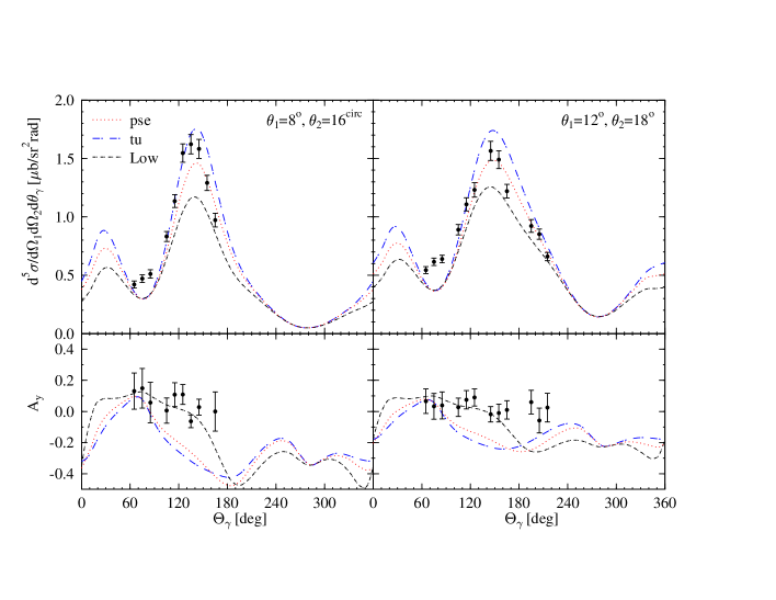
Figure 2: The differential cross section $d^{5}\sigma/d\Omega_{1}d\Omega_{2}d\theta_{\gamma}$ (upper panel) and the analyzing power $A_{y}$ (lower panel) for single-photon bremsstrahlung as functions of the photon angle. Prediction of different SPM’s (see text) are compared with recent data obtained at KVI Hui99 at a beam energy of 190 MeV. The angles of the outgoing protons are kept fixed at $\theta_{1}=8^{\circ}$, $\theta_{2}=16^{\circ}$ (left panel) and $\theta_{1}=12^{\circ}$, $\theta_{2}=18^{\circ}$ (right panel) for coplanar geometry.

In Fig. (2) the results for each of the three soft-photon models are compared with cross-section data obtained in a recent high precision experiment at KVI at 190 MeV incident energy Hui99 . The predictions of the present pse-SPM appear to lie right in between those of Low-SPM and tu-SPM. As such the present SPM appears to be in rather good agreement with the data even though the photon energy is relatively large (about 80 MeV).

Also shown is the analyzing power $A_{y}$ for scattering of the polarized protons. These results suggest that Low-SPM gives a better description of the data Hui99 at 190 MeV than pse-SPM and tu-SPM. The latter models give close results.

II.2 The SPM for two-photon bremsstrahlung

The pse-SPM developed in the above can readily be extended to the case of two-photon bremsstrahlung since no explicit contact terms (which appear in the Low-SPM and in the tu-SPM) were introduced. One therefore does not have to deal with the complication of adding a two-photon contact term or discuss the modification of the single-photon contact term due to the presence of the second photon.

Figure 3: Feynman diagrams included in the calculation of the two-photon bremsstrahlung amplitude.

To obtain the two-photon equivalent of pse-SPM (pse-2SPM) one proceeds in a similar manner as discussed in the previous section. The T-matrix is written in terms of a power-series expansion around the point of average kinematics as given in Eq. (4), where $k^{2}$ now equals $m_{\gamma\gamma}^{2}$, the invariant mass squared of the two-photon system. This particular point is used to preserve antisymmetry of the matrix element (see ref Kor96 ). The amplitude can be constructed by adding the contributions of all diagrams where the two photons (with momenta $q_{1}$ and $q_{2}$, $k=q_{1}+q_{2}$) are attached to the external legs in all possible permutations (see Fig. (3)),

$${\cal M}(seq)^{\mu\nu}=\bar{u}_{\lambda^{\prime}_{1}}(p^{\prime}_{1})\bar{u}_{\lambda^{\prime}_{2}}(p^{\prime}_{2})$$

$$\Big{[}T_{1}\;S^{(1)}(p_{1}-k)\;\Gamma^{\nu(1)}\;S^{(1)}(p_{1}-q_{1})\;\Gamma^{\mu(1)}$$

$$+\mbox{all possible permutations}\Big{]}\;u_{\lambda_{2}}(p_{2})u_{\lambda_{1}}(p_{1})\;,$$ (10)

where only the first diagram of Fig. (3) has been written explicitly. The $(t,u)$ variables specifying the on-shell point at which the T-matrix is evaluated can be easily expressed in terms of the external momenta for each diagram. However, instead of the true T-matrix the power-series expansion Eq. (3) is used. It can be verified that this amplitude satisfies gauge invariance, i.e. $q_{1\mu}{\cal M}(seq)^{\mu\nu}=q_{2\nu}{\cal M}(seq)^{\mu\nu}=0$, for the case of radiation off the two-proton system. The amplitude therefore obeys the low-energy theorem for the two-photon emission Timpr .

Results for the two-photon bremsstrahlung will be presented in a later section together with the results for the virtual-pion amplitude.

III Pion production

The importance of short-range physics for $\pi^{0}$ production in pp scattering was addressed in many references, e.g. Hor94 ; Hai96 ; Ada97 ; Eng96 . It was shown that this process is very sensitive to the short-range component of the NN interaction which in turns reflects in very strong off-shell effects in the T-matrix describing the pp rescattering in the ${}^{1}S_{0}$ final state. This partial wave gives the most important contribution near the pion-production threshold. As a result of the strong off-shell effects the so-called direct pion production is suppressed, and other contributions, such as the $\pi N$ rescattering, heavy-meson exchanges, etc. become crucial to obtain agreement with experiment.

In this paper we have opted for simpler, more phenomenological approach which still relies on the same on-mass-shell T-matrix as used in the photon-bremsstrahlung calculations. The virtual-pion emission and the sequentional two-photon bremsstrahlung are thus described in equivalent models. The pion-production amplitude is calculated using radiation off external legs only while evaluating the T-matrix at a suitably chosen point corresponding to on-shell kinematics. We use a general pion-nucleon vertex

$$\Gamma_{\pi}(k)={G_{\pi}\over 1+\chi}\gamma^{5}\left(\chi+{k/\over 2\,m_{p}}\right)\,,$$ (11)

where $\chi$ specifies the admixture of pseudo-scalar (PS) coupling and $k$ is the pion (outgoing) momentum. The PS component in the vertex is included to effectively account for the reaction mechanisms which are not explicitly present in the model. This issue will be elaborated further on in this section.

As argued in Mey92 ; Han99 the energy dependence of real pion production indicates that the final-state interaction between the emerging nucleons should be accounted for correctly. For this reason the T-matrix is evaluated at an on-shell point corresponding to the same energy, $s$, and the same ratio $R=t/u$ as is appropriate for each of the four diagrams. In should be noticed that for on-shell kinematics the ratio $R$ is directly related to the proton-proton scattering angle. The amplitude which can be read off the diagrams in Fig. (1) (where the photon line is replaced by the pion one) has the form

$${\cal M}_{\pi}=T_{1}\;S^{(1)}(p_{1}-k)\;\Gamma_{\pi}^{(1)}(k)+$$

$$\Gamma_{\pi}^{(1)}(k)\;S^{(1)}(p^{\prime}_{1}+k)\;T_{2}+T_{3}\;S^{(2)}(p_{2}-k)\;\Gamma_{\pi}^{(2)}(k)\;$$

$$+\;\Gamma_{\pi}^{(2)}(k)\;S^{(2)}(p^{\prime}_{2}+k)\;T_{4}$$ (12)

with

$$T_{1}=T(s_{f},R_{1}={t_{2}}/{u_{1^{\prime}2}})\,,\;\;\;T_{2}=T(s_{i},R_{2}={t_{2}}/{u_{12^{\prime}}})\,,$$

$$T_{3}=T(s_{f},R_{3}={t_{1}}/{u_{12^{\prime}}})\,,\;\;\;T_{4}=T(s_{i},R_{4}={t_{1}}/{u_{1^{\prime}2}})\,.$$ (13)

The nucleon spinors in Eq. (12) are omitted for brevity.

In the process of calculating the pion-production cross section we noticed that special care should be paid to the representation of the T-matrix. Initially the calculation was performed by expanding the T-matrix in the usual set of five Lorentz covariants given in Eq. (2).

Changing the ratio $\chi$ of the PS and pseudo-vector (PV) couplings by a mere 0.1 would change the real-pion production cross section by about one order of magnitude. This extreme and unrealistic sensitivity could be traced back to the unrealistically large coupling to negative-energy states in the pp system at small energies which is introduced with this particular choice of covariants. To avoid the aforementioned problem we have therefore introduced another set of Lorentz tensors, chosen such that, when sandwiched between large components of positive-energy spinors, they reduce to the five operators usually taken in a non-relativistic formulation (see for example Gol64 ; Ker59 ; Her95 ),

$$\Omega^{nr}={1,\vec{\sigma}^{(1)}\cdot\vec{\sigma}^{(2)},i(\vec{\sigma}^{(1)}+\vec{\sigma}^{(2)})\cdot\hat{n},S_{12}(\hat{t}),S_{12}(\hat{u})}\;,$$ (14)

where $\vec{n}=(\vec{p}_{1}-\vec{p}_{2})\times(\vec{p^{\prime}}_{1}-\vec{p^{\prime}}_{2})$, $\vec{t}=\vec{q}_{t}$, $\vec{u}=\vec{q}_{u}$, the tensor is given by $S_{12}(\hat{p})=3\;\vec{\sigma}^{(1)}\cdot\hat{p}\;\vec{\sigma}^{(2)}\cdot\hat{p}-\vec{\sigma}^{(1)}\cdot\vec{\sigma}^{(2)}$, and the hat denotes a unit vector. Emphasizing the dependence on $s$ and $R$ of the Lorentz-invariant coefficients $C_{j}$ the on-shell T-matrix is expressed in a similar way as in Eq. (1),

$$T(s,R)=\sum_{j=1}^{5}C_{j}(s,R)\Omega_{j}^{\ (1)}\cdot\Omega^{j(2)}\;.$$ (15)

A possible choice for the covariants $\Omega_{j}$ is

$$\begin{array}[]{lll}\Omega_{1}=Q/\hskip 2.15277pt_{s}\;,&\Omega_{2}=\gamma_{5}Q/\hskip 2.15277pt_{n}\;,&\Omega_{3}=\gamma_{5}Q/\hskip 2.15277pt_{p}\;,\\ \Omega_{4}=\gamma_{5}Q/\hskip 2.15277pt_{k}\;,&\Omega_{5}=\Omega_{2}+\Omega_{1}\;,&\end{array}$$ (16)

defined in terms of the orthogonal four-vectors,

$$\begin{array}[]{l}Q_{s}^{\mu}=(p_{1}^{\mu}+p_{2}^{\mu})/W\;,\\ Q_{k}^{\mu}={\cal N}_{k}(q_{t}^{\mu}-(q_{t}\cdot Q_{s})Q_{s}^{\mu})\;,\\ Q_{p}^{\mu}={\cal N}_{p}(q_{u}^{\mu}-(q_{u}\cdot Q_{s})Q_{s}^{\mu}+(q_{u}\cdot Q_{k})Q_{k}^{\mu})\;,\\ Q_{n}^{\mu}=\epsilon^{\mu\nu\sigma\rho}(Q_{s})_{\nu}(Q_{k})_{\sigma}(Q_{p})_{\rho}\;,\end{array}$$ (17)

normalized such that $Q_{s}^{2}=-Q_{k}^{2}=-Q_{p}^{2}=-Q_{n}^{2}=1$, where $W^{2}=s=(p_{1}+p_{2})^{2}$ and $\ \epsilon^{\mu\nu\sigma\rho}$ is the fully antisymmetric Levi-Civita tensor. The momenta $q_{t}$ and $q_{u}$ are chosen according to Eq. (5). It is straightforward to show that in the pp-CM system the matrix elements of $\Omega_{j}^{\ (1)}\cdot\Omega^{j(2)}$ for the large components of the spinors are indeed a linearly independent combination of the non-relativistic operators given in Eq. (14). The fifth term in Eq. (16), for example, is the only one that, in the non-relativistic reduction, contributes a term like the third one in Eq. (14). In addition the matrix elements between large and small components vanish. This set of five operators is not unique; any linear combination of $q_{t}$ and $q_{u}$ could have been used to define $Q_{k}$ and furthermore $\Omega_{1}=1$ is also a valid choice. We have checked that any of these ambiguities have only minor effects on the calculated pion-production amplitude.

With the covariants in Eq. (16) the cross section for real-pion production still depends on the ratio $\chi$ but in a much more gentle way. By varying $\chi$ and keeping a realistic $\pi N$ coupling constant, the experimentally measured cross section can be reproduced with $\chi=1.05$. For $\chi=0$, corresponding to the pure PV coupling, the cross section is about a factor 10 larger than experiment and appears to be independent of the choice of covariants, Eq. (2) or Eq. (16). The latter feature is probably due to the fact that for a PV coupling the contribution of negative-energy states is suppressed.

To understand the sensitivity of the cross section to the PS component in the $\pi N$ vertex we can rewrite the pion-production amplitude in the form

$${\cal M}_{\pi}={\cal M}_{\pi}^{(PV)}+{\cal M}_{\pi}^{(cont)}\,,$$ (18)

where the purely PV contribution is

$${\cal M}_{\pi}^{(PV)} = i\frac{G_{\pi}}{2m_{p}}\Big{[}T_{1}\,\gamma_{5}^{(1)}\Big{(}1-\frac{m_{p}k/^{(1)}}{k\cdot p_{1}-m_{\pi}^{2}/2}\Big{)}$$ (19)

$$+\Big{(}1-\frac{m_{p}k/^{(1)}}{k\cdot p^{\prime}_{1}+m_{\pi}^{2}/2}\Big{)}\gamma_{5}^{(1)}\,T_{2}$$

$$+T_{3}\,\gamma_{5}^{(2)}\Big{(}1-\frac{m_{p}k/^{(2)}}{k\cdot p_{2}-m_{\pi}^{2}/2}\Big{)}$$

$$+\Big{(}1-\frac{m_{p}k/^{(2)}}{k\cdot p^{\prime}_{2}+m_{\pi}^{2}/2}\Big{)}\gamma_{5}^{(2)}\,T_{4}\Big{]}\,,$$

and ${\cal M}_{\pi}^{(cont)}$ has a form of a 5-point contact vertex,

$${\cal M}_{\pi}^{(cont)} = -i\Big{(}\frac{\chi}{1+\chi}\Big{)}\frac{G_{\pi}}{2m_{p}}\Big{(}T_{1}\,\gamma_{5}^{(1)}+\gamma_{5}^{(1)}\,T_{2}$$ (20)

$$+T_{3}\,\gamma_{5}^{(2)}+\gamma_{5}^{(2)}\,T_{4}\Big{)}\,.$$

The important observation is that in the soft-pion limit ($k\to 0$) the amplitude ${\cal M}_{\pi}^{(PV)}$ fulfills the requirement of the chiral symmetry Nam62 (to be precise, the limit in Eq. (19) shoud be taken in the order: $\lim_{m_{\pi}\to 0}\{\lim_{\vec{k}\to 0}...\}$). In this case, of course, $T_{1}=T_{2}=T_{3}=T_{4}$ is the T-matrix calculated in kinematics of on-shell pp scattering. However the pion mass is finite, and the T-matrices in the dominant diagrams, $T_{1}$ and $T_{3}$, corresponding to the pion emission off the initial legs, in fact should enter far off-shell (for example, the corresponding off-energy-shell CM momentum is about ${(m_{\pi}m_{p})}^{1/2}\approx 370$ MeV). Due to a strong off-shell dependence of the T-matrix (see, e.g. Hai96 ; Her95 ) a sizable reduction of the cross section calculated only with ${\cal M}_{\pi}^{(PV)}$ should occur. The contact term in Eq. (20) effectively accounts for this effect, as well as the other important mechanisms which act in the opposite direction, such as (off-shell) $\pi N$ rescattering and heavy-meson exchanges, and possible genuine contact vertices in the underlying Lagrangian. We will consider $\chi$ as a phenomenological parameter of the model.

Our approach has a certain similarity to the soft-pion model of ref. Sch69 , where the authors applied yet another method to account for off-shell effects, and found a reasonable agreement with the data available at the time.

Figure 4: The angle-integrated cross section for real-pion production is plotted versus the relative kinetic energy $T_{12}$ of the outgoing two-proton system. Results are shown for two incoming proton energies and for a selection of $\pi$-N relative kinetic energies.

The angle integrated cross section for real-$\pi^{0}$ production is plotted in Fig. (4) as function of the relative kinetic energy in the final two-proton system, defined as $T_{12}=M_{12}-2m_{p}$, where $M_{12}$ is the invariant mass of the two-proton system. It can be seen that to a large extent the cross section is independent of $T_{23}=M_{23}-m_{p}-m_{\pi}$ and falls off roughly proportional to $1/T_{12}$ in accordance with Mey92 .

Figure 5: The integrated cross section for real-pion production as function of $\eta$ which is related to the beam energy through Eq. (35). The data are from Mey92 .

The total $\pi^{0}$ production cross section as function of $\eta$ (see Eq. (35) for the definition) is compared to the data of Mey92 in Fig. (5). It is seen that the calculation agrees well with the data in both magnitude and energy dependence. As such we conclude that this simple model is able to give a reasonable estimate of the pion-production cross section and will thus use it also in the calculation of virtual-pion production discussed in the following section.

III.1 Virtual pions

The amplitude for two-photon emission mediated by a virtual pion can be factorized in two terms. The first is the amplitude for virtual-pion production, ${\cal M}_{\pi}$, which is identical in structure to the one for real pions. The second term describes the decay of the virtual pion. The amplitude in question now reads

$${\cal M}^{\mu\nu}({\pi}) = \frac{ie^{2}g_{\pi\gamma\gamma}}{(k^{2}-m^{2}_{\pi}+i0)m_{\pi}}\epsilon^{\mu\nu\alpha\beta}q_{1\alpha}q_{2\beta}$$ (21)

$$\times{\cal M}_{\pi}(p^{\prime}_{1},p^{\prime}_{2};p_{1},p_{2})\;,$$

where $k=q_{1}+q_{2}$ is the momentum of the virtual pion and $g_{\pi\gamma\gamma}\approx 0.0375$ is the $\pi^{0}\rightarrow\gamma\gamma$ decay constant. The total amplitude for the $pp\to pp\gamma\gamma$ process is

$${\cal M}^{\mu\nu}={\cal M}^{\mu\nu}(seq)+{\cal M}^{\mu\nu}(\pi)\;,$$ (22)

the sum of the amplitudes given in Eq. (10) and Eq. (21)

IV Results

The calculations presented in this section are done for an incoming proton energy of 280 MeV in the Lab system which is just below the pion-production threshold ($2m_{\pi}+m_{\pi}^{2}/2m_{p}$).

Figure 6: The dependence of the differential cross section $d^{8}\sigma/dm_{\gamma\gamma}dM^{2}_{12}dM^{2}_{23}d\Omega_{\gamma\gamma}d\Omega_{k}d\phi_{1}$ on the two-photon angles. The two-photon bremsstrahlung result is given by the dense-dotted curve, the pure virtual-pion process by the sparse-dotted curve, the full result by the drawn curve, while the dashed curve gives the coherent sum when changing ad-hoc the sign of the virtual-pion contribution.

In Fig. (6) the cross section for two-photon production is plotted for certain exclusive kinematics. We have opted to use the Dalitz coordinates (see Appendix B for a more detailed discussion) for expressing the differential cross sections, specified by i) $T_{12}$, the relative energy between the two protons; ii) $T_{13}$, the relative energy between a proton and the sum-momentum of the two photons (equal to the momentum of the virtual pion); iii) the Euler angles of the plane spanned by the two protons and the virtual pion with respect to the incoming beam direction, i.e. ($\theta_{k},\phi_{k}$), and where the third angle is trivial due to azimuthal symmetry. This is supplemented by the angles ($\theta_{\gamma\gamma},\phi_{\gamma\gamma}$) specifying the orientation of the two-photon relative momentum in their c.m. frame and the invariant mass $m_{\gamma\gamma}$ of the two-photon system or -equivalently- the virtual pion. These coordinates can be used for the sequential two-photon emission as well as for the virtual-pion process. We have used these coordinates instead of the traditionally adopted ones in bremsstrahlung for a few reasons. Firstly, the phase space factor is a very smooth (in many cases independent) function of the kinematical variables and differential cross sections thus directly reflect the magnitude of the underlying matrix element. Secondly, the absence of divergencies of the phase space factor allows for a straightforward evaluation of (partially) integrated cross sections. Thirdly, these coordinates uniquely determine the kinematics of the event while in polar coordinates a kinematical solution is not always uniquely defined (this happens in very selected parts of phase space only). It should be noted that $T_{23}$ is related to $T_{12}$ and $T_{13}$ by a simple algebraic relation.

In the figures the two-photon cross sections due to the intermediate virtual-$\pi^{0}$ mechanism and the sequential two-photon emission are indicated separately. There is a strong interference between the two contributions, the total (from adding the amplitudes, labelled ’tot+’ in the figures) is larger than the sum of the individual cross sections. The importance of interference for the total cross section implies that the cross section is sensitive to the relative phase between the amplitudes of the uncorrelated and the virtual-pion two-photon emission processes. To show this, we also plot the cross section for the case in which the virtual-pion matrix element has been arbitrarily, only for display purposes, multiplied with a minus sign (i.e. changing the relative sign in Eq. (22) eventhough the sign given there is correct). This calculation, labeled ’tot-’ in Fig. (6), gives rise to a much smaller total cross section. It should be noted that changing the sign does not affect the real-pion production cross section since it is independent of the sign. From Fig. (6) it can be seen that the angular distributions depend on the phase of the virtual-pion contribution, however the largest effect of changing the sign shows up in the overall magnitude. We have checked that this is the case in a large region of phase space and the distributions shown here can be regarded as typical.

Another aspect which can be seen from Fig. (6) is that the angular distributions of the sequentional two-photon emission process show pronounced structures. This is to be expected as the single-photon bremsstrahlung angular distribution shows pronounced peaks which are due to the quadrupole nature of the electric radiation and the interference with magnetic radiation. The virtual-pion mechanism has a rather featureless distributions, due to the fact that the two photons couple to the quantum numbers of the pion, $J^{\pi}=0^{-}$.

It is also apparent from Fig. (6) that –unfortunately– one cannot point to a particular feature in the angular distribution which is especially sensitive to the virtual-pion contribution. There are no quantum numbers that distinguish this process from the bremsstrahlung contribution.

For the above reason, and also because cross sections are –in general– small for two-photon emission, we investigate whether the virtual-pion signal can also be seen in less exclusive kinematics where certain angles have been integrated. Since, as remarked before, the virtual pion contribution seems to give primarily rise to an overall increase of the cross sections we have performed a simple integration of the differential cross section.

Figure 7: The cross section for two-photon production, integrated over angles, is plotted versus the relative kinetic energy $T_{12}$ of the final two-proton system. Results are shown for a selection of $\pi$-N relative kinetic energies. The meaning of the curves is the same as in Fig. (6). The end points of the curves are determined by kinematics.

The squared matrix element for pion emission is inversely proportional to the relative energy in the final pp system Mey92 . One thus expects that the virtual-pion process is most pronounced for the lowest values of $T_{12}$. This is indeed supported by our calculations as shown in Fig. (7), where the difference between the full calculation (labeled ’tot+’) and the sequential two-photon process strongly depends on $T_{12}$ and hardly on $T_{23}$. In Fig. (7) all angles have been integrated.

Figure 8: The cross section for two-photon production, integrated over all variables at fixed relative kinetic energy $T_{12}=3$ MeV of the final two-proton system, is plotted as function of the two-photon invariant mass. The meaning of the curves is the same as in Fig. (6).

The unambiguous signature of the virtual-pion contribution is that it increases the closer one approaches the real-pion pole. This can clearly be seen from Fig. (8) where the cross section is shown as function of $m_{\gamma\gamma}$ at fixed $T_{12}$. All other variables, i.e. all angles and also $T_{23}$, are integrated. Even this rather inclusive cross section shows a clear sensitivity to the interference between the sequential and the virtual-pion two-photon emission processes.

V Summary and conclusions

In this work we have shown that the two-photon bremsstrahlung offers the interesting possibility to ‘measure’ subthreshold pion production in $pp$ scattering. It allows for studying pion production in kinematics which is not accessible in the $pp\rightarrow pp\pi^{0}$ reaction. In addition, the phase of the virtual-pion process with respect to that of sequential two-photon emission can be investigated.

To account for the sequential two-photon emission process, which is an important background, a novel soft-photon model (called pse-SPM) is developed. This model is tested in a calculation of single-photon bremsstrahlung, and is shown to give accurate results for cross sections.

Calculated exclusive cross sections of the $pp\rightarrow pp\gamma\gamma$ reaction are in general small, however sensitivity of the cross sections to the virtual-pion signal remains even for rather inclusive cross sections.

Appendix A Kinematics for two-photon production

For the reaction $\ N+N\rightarrow N+N+\gamma+\gamma$ the momenta are denoted by $\ p_{1},p_{2},p_{1}^{\prime},p_{2}^{\prime},q_{1},q_{2}$ (see Fig. (3)). Energy-momentum conservation reads  $p_{1}+p_{2}=p_{1}^{\prime}+p_{2}^{\prime}+q_{1}+q_{2}$. The cross section is

$$d\sigma = \frac{m_{p}^{4}}{j}\int|A|^{2}(2\pi)^{4}\delta^{4}(p_{1}+p_{2}-p_{1}^{\prime}-p_{2}^{\prime}-q_{1}-q_{2})$$

$$\times\frac{d^{3}p_{1}^{\prime}}{(2\pi)^{3}E_{1}^{\prime}}\frac{d^{3}p_{2}^{\prime}}{(2\pi)^{3}E_{2}^{\prime}}\frac{d^{3}q_{1}}{(2\pi)^{3}2\varepsilon_{1}}\frac{d^{3}q_{2}}{(2\pi)^{3}2\varepsilon_{2}}\,,$$

where $A={\cal M}^{\mu\nu}\epsilon^{*}_{1\mu}\epsilon^{*}_{2\nu}$ is the invariant amplitude, $\epsilon_{1}$ and $\epsilon_{2}$ are the polarization vectors of the photons, $\varepsilon_{1}=|\vec{q}_{1}|$, $\varepsilon_{2}=|\vec{q}_{2}|$, and $j=\sqrt{(p_{1}\cdot p_{2})^{2}-m_{p}^{4}}=m_{p}|\vec{p}_{Lab}|$ in the laboratory frame where $p_{2}=(m_{p},\vec{0})$. Using the identity $\int\delta^{4}(q_{1}+q_{2}-k)d^{4}k=1$ the cross section is put in the form

$$d\sigma = \frac{m_{p}^{4}}{(2\pi)^{8}j}\int|A|^{2}\delta^{4}(p_{1}+p_{2}-p_{1}^{\prime}-p_{2}^{\prime}-k)I_{\gamma\gamma}$$ (23)

$$\times\frac{d^{3}p_{1}^{\prime}}{E_{1}^{\prime}}\frac{d^{3}p_{2}^{\prime}}{E_{2}^{\prime}}d^{4}k\,,$$

where $I_{\gamma\gamma}$ is the two-photon phase-space integral defined as

$$I_{\gamma\gamma}=\int\delta^{4}(q_{1}+q_{2}-k)\frac{d^{3}q_{1}}{2\varepsilon_{1}}\frac{d^{3}q_{2}}{2\varepsilon_{2}}\,.$$

To calculate this integral in an arbitrary frame we introduce the relative and total 4-momenta of the photons

$$k=q_{1}+q_{2},\;\;\;\;\;\;l=\frac{1}{2}(q_{1}-q_{2}),$$

$$q_{1}=\frac{1}{2}k+l,\;\;\;\;\;\;q_{2}=\frac{1}{2}k-l\,.$$ (24)

The Jacobian of the transformation from $\vec{q}_{1},\ \vec{q}_{2}$ to $\vec{l},\ \vec{k}$ is unity, and after removing the trivial $\delta$-function we get

$$I_{\gamma\gamma} = \int\delta(\varepsilon_{\frac{1}{2}\vec{k}+\vec{l}}+\varepsilon_{\frac{1}{2}\vec{k}-\vec{l}}-k_{0})\frac{d^{3}l}{2\varepsilon_{\frac{1}{2}\vec{k}+\vec{l}}\,2\varepsilon_{\frac{1}{2}\vec{k}-\vec{l}}}\,$$ (25)

$$= \frac{|\vec{l}|^{2}}{4(|\vec{l}|k_{0}-|\vec{k}|l_{0}\cos\theta_{\gamma\gamma})}d\Omega_{\gamma\gamma}\,,$$

with $d\Omega_{\gamma\gamma}=\sin\theta_{\gamma\gamma}d\theta_{\gamma\gamma}d\phi_{\gamma\gamma}$, where we introduced the polar and azimuthal angles $\theta_{\gamma\gamma}$ and $\phi_{\gamma\gamma}$ between the 3-vectors $\vec{k}$ and $\vec{l}$. For real photons ($q_{1}^{2}=q_{2}^{2}=0$) one can show that $k\cdot l=0$ and $4\,l^{2}+m_{\gamma\gamma}^{2}=0$, where $m_{\gamma\gamma}^{2}=k^{2}$ is the invariant mass of the two-photon system. Expressing now $l_{0}$ in terms of the 3-momentum $|\vec{l}|$ we obtain

$$|\vec{l}|=\frac{m_{\gamma\gamma}}{2\sqrt{1-\frac{\vec{k}^{2}}{k_{0}^{2}}\cos^{2}\theta_{\gamma\gamma}}}=\frac{m_{\gamma\gamma}k_{0}}{2\sqrt{m_{\gamma\gamma}^{2}+\vec{k}^{2}\sin^{2}\theta_{\gamma\gamma}}},$$

with $k_{0}=\sqrt{m_{\gamma\gamma}^{2}+\vec{k}^{2}}.$ The two-photon phase space Eq. (25) can be simplified to

$$I_{\gamma\gamma}=\frac{|\vec{l}|^{3}}{k_{0}m_{\gamma\gamma}^{2}}d\Omega_{\gamma\gamma}\,.$$ (26)

As a last step the integration over $k_{0}$ in Eq. (23) is replaced by an integration over the two-photon invariant mass using $k_{0}dk_{0}=m_{\gamma\gamma}dm_{\gamma\gamma}$. We obtain

$$d\sigma=\frac{2m_{p}^{4}}{(2\pi)^{8}j}\int|A|^{2}J(m_{\gamma\gamma})I_{\gamma\gamma}m_{\gamma\gamma}dm_{\gamma\gamma}\,,$$ (27)

where we introduced the 3-particle phase-space integral

$$J(m_{\gamma\gamma}) = \int\delta^{4}(p_{1}+p_{2}-p_{1}^{\prime}-p_{2}^{\prime}-k)$$ (28)

$$\times\frac{d^{3}p_{1}^{\prime}}{E_{1}^{\prime}}\frac{d^{3}p_{2}^{\prime}}{E_{2}^{\prime}}\frac{d^{3}k}{2k_{0}}\,.$$

In the one-photon bremsstrahlung the similar integral is traditionally evaluated in polar coordinates (see, for example, Kor96 ) leading to the cross section of the type shown in Fig. (2). For the two-photon bremsstrahlung in the present paper we will use the Dalitz coordinates instead, as discussed in Appendix B.

Appendix B Dalitz coordinates

To evaluate the phase-space integral in Eq. (28) we choose the CM frame where $\vec{p}_{1}+\vec{p}_{2}=0$, and carry out the integration over $\vec{p}_{2}^{\,\prime}$. Introducing $s=(p_{1}+p_{2})^{2}$ we obtain

$$J(m_{\gamma\gamma})=\int\delta(\sqrt{s}-E_{1}^{\prime}-E_{2}^{\prime}-k_{0})\frac{d^{3}p_{1}^{\prime}}{E_{1}^{\prime}E_{2}^{\prime}}\frac{d^{3}k}{2k_{0}}\,,$$

where $E_{2}^{\prime 2}=m_{p}^{2}+\vec{p}_{2}^{\,\prime 2}=m_{p}^{2}+(\vec{p}_{1}^{\,\prime}+\vec{k})^{2}=m_{p}^{2}+\vec{p}_{1}^{\,\prime 2}+\vec{k}^{2}+2p_{1}^{\prime}k\cos\theta_{13}$. Using

$$d^{3}p_{1}^{\prime}\,d^{3}k=p_{1}^{\prime}\,E_{1}^{\prime}\,dE_{1}^{\prime}\,d\Omega_{1}\,k\,k_{0}\,dk_{0}\,d\Omega_{k}$$

$$=p_{1}^{\prime}\,E_{1}^{\prime}\,dE_{1}^{\prime}\,d\cos\theta_{13}\,d\phi_{1}\,k\,k_{0}\,dk_{0}\,d\cos\theta_{k}\,d\phi_{k}$$

and integrating over $\cos\theta_{13}$ using the $\delta$-function we obtain

$$J(m_{\gamma\gamma})={1\over 2}d\cos\theta_{k}\,d\phi_{k}\,d\phi_{1}\,dk_{0}\,dE_{1}^{\prime}\;.$$

Defining invariant masses

$$M_{12}^{2} = (T_{12}+2m_{p})^{2}=(p_{1}^{\prime}+p_{2}^{\prime})^{2}$$

$$= s-2\sqrt{s}k_{0}+m_{\gamma\gamma}^{2}\;,$$

$$M_{23}^{2} = (T_{23}+m_{p}+m_{\pi})^{2}=(p_{2}^{\prime}+k)^{2}$$ (29)

$$= s-2\sqrt{s}E_{1}^{\prime}+m_{p}^{2},$$

we can cast the integral $J(m_{\gamma\gamma})$ in the form

$$J(m_{\gamma\gamma})={1\over 8s}d\cos\theta_{k}\,d\phi_{k}\,d\phi_{1}\,d\,M_{12}^{2}dM_{23}^{2}\,.$$ (30)

Here the angles $\phi_{k},\,\theta_{k},\,\phi_{1}$ describe in the CM frame the orientation of the plane in which the momenta lie of the outgoing two protons and the two-photon system (the virtual pion) with respect to the incoming beam. Specifically, the angle $\phi_{1}$ is defined as the azimuthal angle of the momentum $\vec{p}_{1}^{\,\prime}$ in the frame, where momentum $\vec{k}$ is along OZ axis and the OX axis lies in the plane spanned by the beam and $\vec{k}$. The angle $\theta_{k}$ is taken as the angle in the CM frame between the incoming momentum and $\vec{k}$ while $\phi_{k}$ is a trivial azimuthal angle. In the CM frame the momenta can now be expressed as

$$\vec{k}=(k_{x},\;k_{y},\;k_{z})=k(\sin\theta_{k},\;0,\;\cos\theta_{k}),\,$$

$$\vec{p}_{1}^{\,\prime}=(p_{1x}^{\prime},\;p_{1y}^{\prime},\;p_{1z}^{\prime})=$$

$$=p_{1}^{\prime}(\cos\theta_{k}\sin\theta_{13}\cos\phi_{1}+\sin\theta_{k}\cos\theta_{13},$$

$$\;\sin\theta_{13}\sin\phi_{1},\;-\sin\theta_{k}\sin\theta_{13}\cos\phi_{1}+\cos\theta_{k}\cos\theta_{13}),$$

$$\vec{p}_{2}^{\,\prime}=-\vec{p}_{1}^{\,\prime}-\vec{k}.$$

The magnitudes of $\vec{k}$, $\vec{p}_{1}^{\,\prime}$ and $\vec{p}_{2}^{\,\prime}$ are determined through the energies of the two-photon system and nucleons

$$k_{0} = \frac{s-M_{12}^{2}+m_{\gamma\gamma}^{2}}{2\sqrt{s}}\;,$$

$$E_{1}^{\prime} = \frac{s-M_{23}^{2}+m_{p}^{2}}{2\sqrt{s}}\;,$$

$$E_{2}^{\prime} = \sqrt{s}-E_{1}^{\prime}-k_{0}\,,$$

and the angle between $\vec{p}_{1}^{\,\prime}$ and $\vec{k}$ can be expressed as,

$$\cos\theta_{13}=(E_{2}^{\prime 2}-E_{1}^{\prime 2}-k_{0}^{2}+m_{\gamma\gamma}^{2})/{2kp_{1}^{\prime}}.$$

So far the momenta were defined in the CM frame. The boost to the Lab system is specified by the velocity $V={p_{1}}/({m_{p}+E_{1}})$ and the Lorentz-factor $\gamma=({m_{p}+E_{1}})/{\sqrt{s}}$. The Z components of the vectors in the lab can now be expressed as

$$k_{z}^{Lab} = \gamma(k_{z}+Vk_{0}),$$

$$p_{1z}^{\prime Lab} = \gamma(p_{1z}^{\prime}+VE_{1}^{\prime}),$$

$$p_{2z}^{\prime Lab} = p_{1}-k_{z}^{Lab}-p_{1z}^{\prime Lab},$$

while the X and Y components do not change.

Appendix C Total cross section for pion production

Using the Dalitz coordinates, the cross section for real pion production is written as

$$d\sigma=\frac{m_{p}^{4}}{(2\pi)^{5}j}|{\cal M}_{\pi}|^{2}J(m_{\pi})$$ (31)

where particle 3 is associated with the pion and $J(m_{\pi})$ is given in Eq. (30) where $m_{\gamma\gamma}\to m_{\pi}$.

Let us first make a tentative assumption that the amplitude is a constant and integrate the cross section in Eq. (31) over angles,

$$d\sigma=\frac{m_{p}^{4}\pi^{2}}{(2\pi)^{5}js}|{\cal M}_{\pi}|^{2}\,dM_{12}^{2}\,dM_{23}^{2}\;.$$ (32)

For the total cross section we integrate over invariant masses

$$\sigma=\frac{m_{p}^{4}\pi^{2}}{(2\pi)^{5}js}|{\cal M}_{\pi}|^{2}I(s)\,,$$ (33)

where we introduced the integral

$$I(s) = \int_{{M_{12}^{min}}^{2}}^{{M_{12}^{max}}^{2}}\,\Big{(}\int_{{M_{23}^{min}}^{2}}^{{M_{23}^{max}}^{2}}dM_{23}^{2}\Big{)}\,dM_{12}^{2}$$ (34)

$$= 2\int_{M_{12}^{min}}^{M_{12}^{max}}\sqrt{(M_{12}^{2}-4m_{p}^{2})}$$

$$\times\sqrt{(s-m_{\pi}^{2}-M_{12}^{2})^{2}-4m_{\pi}^{2}M_{12}^{2}}\,dM_{12}\,,$$

with the lower and upper limits $M_{12}^{min}=2m_{p}$ and $M_{12}^{max}=\sqrt{s}-m_{\pi}$ respectively. At the upper limit the pion 3-momentum in the CM system, $\vec{k}^{2}={\left(M_{12}^{2}-(\sqrt{s}-m_{\pi})^{2}\right)\left(M_{12}^{2}-(\sqrt{s}+m_{\pi})^{2}\right)/4s}\;,$ vanishes while it reaches a maximum at the lower limit,

$$\vec{k}^{2}_{max}=m_{\pi}^{2}\eta^{2}=b(b+4m_{\pi}\sqrt{s})/4s$$ (35)

which defines the conventionally used variable $\eta$ Mey92 in terms of $b=(\sqrt{s}-m_{\pi})^{2}-4m_{p}^{2}$. Introducing the relative $pp$ 3-momentum $4\vec{p}^{2}=\left(M_{12}^{2}-4m_{p}^{2}\right)$ the phase space integral Eq. (34) can also be put in the familiar form $I(s)=\int 16|\vec{p}||\vec{k}|\sqrt{s/M_{12}^{2}}d\vec{p}^{2}$.

With the substitutions $t=(M_{12}^{2}-4m_{p}^{2})/b$, $a=4m_{p}^{2}$ and $c=(\sqrt{s}+m_{\pi})^{2}-4m_{p}^{2}$ the phase space integral Eq. (34) can be cast in the form

$$I(s)=b^{2}\int_{0}^{1}dt\sqrt{t(t-1)(t-c/b)\over(t+a/b)}\;.$$ (36)

This shows that the total cross section is roughly proportional to $b^{2}$ and thus proportional to $\eta^{4}$ at low energies, in contrast to the data. It has been argued in Mey92 that the assumption made that the matrix element is constant is not valid. The pion-emission process is strongly affected by the final-state NN interaction at low energies, the effect of which is roughly proportional to $1/\vec{p}^{2}=4/t\,b$. Including this factor in the integrand gives a total cross section proportional to $\eta^{2}$, in rough agreement with the data (above $\eta=0.2$). The approach that we chose for evaluating the amplitude and comparison with experiment are described in detail in sect. III.

References

- (1) R.A. Stallwood, R.B. Sutton, T.H. Fields, J.G. Fox, and J.A. Kane, Phys. Rev. 109, 1716 (1958).
- (2) F. Hachenberg and H.J. Pirner, Ann. Phys. 112, 401 (1978).
- (3) H.O. Meyer et al., Phys. Rev. Lett. 65, 2846 (1990); H.O. Meyer, C. Horowitz, H. Nann, P.V. Pancella, S.F. Pate, R.E. Pollock, B. Von Przewoski, T. Rinckel, M.A. Ross, and F. Sperisen, Nucl. Phys. A 539, 633 (1992).
- (4) A. Bondar et al., Phys. Lett. B 356, 8 (1995).
- (5) G.A. Miller and P.U. Sauer, Phys. Rev. C 44, R1725 (1991).
- (6) J.A. Niskanen, Phys. Lett. B 289, 227 (1992).
- (7) T.-S.H. Lee and D.O. Riska, Phys. Rev. Lett. 70, 2237 (1993).
- (8) C.J. Horowitz, H.O. Meyer, and D.K. Griegel, Phys. Rev. C 49, 1337 (1994).
- (9) E. Hernandez and E. Oset, Phys. Lett. B 350, 158 (1995).
- (10) J. Adam Jr., A. Stadler, M.T. Peña, and F. Gross, Phys. Lett. B 407, 97 (1997).
- (11) U. Van Kolck, G.A. Miller, and D.O. Riska, Phys. Lett. B 388, 679 (1996).
- (12) T. Sato, T.-S.H. Lee, F. Myhrer, and K. Kubodera, Phys. Rev. C 56, 1246 (1997).
- (13) A. Engel, R. Shyam, U. Mosel, and A.K. Dutt-Mazumder, Nucl. Phys. A 603, 387 (1996).
- (14) C. Hanhart, J. Haidenbauer, O. Krehl, and J. Speth, Phys. Lett. B 444, 25 (1998); C. Hanhart, J. Haidenbauer, O. Krehl, and J. Speth, Phys. Rev. C 61, 064008 (2000).
- (15) B.-Y. Park, F. Myhrer, J.R. Morones, T. Meissner, and K. Kubodera, Phys. Rev. C 53, 1519 (1996).
- (16) T.D. Cohen, J.L. Friar, G.A. Miller, and U. van Kolck, Phys. Rev. C 53, 2661 (1996).
- (17) E. Gedalin, A. Moalem, and L. Razdolskaya, Phys. Rev. C 60, 031001 (99).
- (18) F. Low, Phys. Rev. 110, 974 (1958).
- (19) E. Nyman, Phys. Rev. 170, 1628 (1968).
- (20) H.W. Fearing, Nucl. Phys. A463, 95 (1987); R.L. Workman and H.W. Fearing, Phys. Rev. C 34, 780 (1986).
- (21) M.K. Liou, D. Lin and B.F. Gibson, Phys. Rev. C 47, 973 (1993).
- (22) M. Liou, R. Timmermans, and B. Gibson, Phys. Lett. B 345, 372 (1995).
- (23) H. Huisman, Ph.D. Thesis, KVI, Groningen (1999); H. Huisman et al., Phys. Rev. Lett. 83, 4017 (1999); ibid, Phys. Lett. B 476, 9 (2000).
- (24) A.S. Khrykin, V.F. Boreiko, Yu.G. Budyashov, S.B. Gerasimov, N.V. Khomutov, Yu.G. Sobolev, and V.P. Zorin, Phys. Rev. C 64, 034002 (2001).
- (25) A. Korchin, O. Scholten, and D. Van Neck, Nucl. Phys. A 602, 423 (1996).
- (26) R. Timmermans, private communication.
- (27) J. Haidenbauer, Ch. Hanhart and J. Speth, Acta. Phys. Polon. B27, 2893 (1996).
- (28) C. Hanhart, K. Nakayama, Phys. Lett. B 454, 176 (1999) and nucl-th/9809059.
- (29) M.L. Goldberger, M.T. Grisaru, S.W. MacDowell and D.Y. Wong, Phys. Rev. 120, 2250 (1960).
- (30) J.A. McNeil, L.R. Ray and S.J. Wallace, Phys. Rev. C 27, 2123 (1983).
- (31) M.L. Goldberger and K.M. Watson, Collision Theory, (Wiley, New York, 1964).
- (32) A.K. Kerman, H. McManus and R.M. Thaler, Ann. of Phys. 8, 551 (1959).
- (33) V. Herrmann, K. Nakayama, O. Scholten, and H. Arellano, Nucl. Phys. A582, 568 (1995).
- (34) K. Nakayama, private communication.
- (35) Y. Nambu and D. Lurié, Phys. Rev. 125, 1429 (1962); Y. Nambu and E. Shrauner, Phys. Rev. 128, 862 (1962).
- (36) M.E. Schillaci, R.R. Silbar and J.E. Young, Phys. Rev. 179, 1261 (1969).