Compton Scattering on the Proton.

Abstract

A microscopic coupled-channels model for Compton and pion scattering off the nucleon is introduced which is applicable at the lowest energies (polarizabilities) as well as at GeV energies. To introduce the model first the conventional K-matrix approach is discussed to extend this in a following chapter to the “Dressed K-Matrix” model. The latter approach restores causality, or analyticity, of the amplitude to a large extent. In particular, crossing symmetry, gauge invariance and unitarity are satisfied. The extent of violation of analyticity (causality) is used as an expansion parameter.

I Introduction

In a K-matrix approach an infinite series of rescattering loops is taken into account with the approximation of incorporating only the pole contributions of the loop diagrams. In this approximation lies both the strong and the weak sides of this approach. By including only the pole contributions, which correspond to rescattering via physical states, unitarity in obeyed and the infinite series can be expressed as a geometric series and summed as given in Eq. (1). Such an approach can be formulated in a co-variant approach, where electromagnetic-gauge invariance is obeyed through the addition of appropriate contact terms. It can also be shown that crossing symmetry is obeyed. In the structure of the kernel a large number of resonances can be accounted for. The weak point of including only the pole contributions of the loop corrections (i.e. only the imaginary part of the loop integrals) is that the resulting amplitude violates analyticity constraints and thus causality.

In Section IV an extension of the K-matrix model is discussed where, without violating the other symmetries, an additional constraint, that of analyticity (or causality), is incorporated approximately. In this approach, called the “Dressed K-Matrix Model”, dressed self-energies and form factors are included in the K-matrix. These functions are calculated self-consistently in an iteration procedure where dispersion relations are used at each recursion step to relate real and imaginary parts.

II The K-Matrix approach

In K-matrix models the T-matrix is written in the form,

$${\mathcal{T}}=(1-Ki\delta)^{-1}\,K\;,$$ (1)

where $\delta$ indicates that the intermediate particles have to be taken on the mass shell and all physics is put in the kernel, the K-matrix. This amounts to re-sum an infinite series of pole contributions ofloop corrections. It is straightforward to check that $S=1+2i{\mathcal{T}}$ is unitary provided that the kernel $K$ is Hermitian. Since Eq. (1) involves integrals only over on-shell intermediate particles, it reduces to a set of algebraic equations when one is working in a partial wave basis. When both the $\pi-N$ and $\gamma-N$ channels are open, the coupled-channel K-matrix becomes a $2\times 2$ matrix in the channel space, i.e.

$$K=\left[\begin{array}[]{cc}K_{\gamma\gamma}&K_{\gamma\pi}\\ K_{\pi\gamma}&K_{\pi\pi}\end{array}\right].$$ (2)

It should be noted that due to the coupled channels nature of this approach the widths of resonances are generated dynamically.

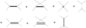
Figure 1: The sum of diagrams included in the K matrix for Compton scattering. A full spectrum of baryon resonances has been included.

In traditional K-matrix models the kernel, the K-matrix, is built from tree-level diagramsGou94 ; Sch96 ; Feu98 ; Kor98 . In the present investigation the type of diagrams included in $K_{\gamma\gamma}$ are similar to that of ref. Kor98 except that the $\Delta$ is treated now as a genuine spin-3/2 resonance Pas01 in order to be compatible with the later treatment of the in-medium $\Delta$ resonance. This K-matrix is indicated in Fig. (1). Most of the (non-strange) resonances below 1.7 GeV have been included. The different coupling constants were fitted to reproduce pion scattering, pion photoproduction and Compton scattering on the nucleon. A comparable fit to the data as in ref. Kor98 could be obtained. In Fig. (2) the results for Compton scattering are compared to data.

Figure 2: The calculated cross section for Compton scattering off the proton as a function of angle at fixed photon energy, and as a function of photon energy at fixed angle. Data are taken from ref. Hal93 .

III Basic symmetries

A realistic scattering amplitude for a particular process should obey certain symmetry relations, such as Unitarity, Covariance, Gauge invariance, Crossing and Causality. In the following each of these symmetries will be shortly addressed, stating its physical significance. It is also indicated which of these is obeyed by the K-matrix approach discussed in the previous section. The comparative success of the K-matrix formalism can be regarded as due to the large number of symmetries which are being obeyed. A violation of anyone of these symmetries will directly imply some problems in applications. Improvements are thus important.

III.1 Unitarity

The unitarity condition for the scattering matrix $S$ reads $S^{\dagger}S=1$. Usually one works with the $T$-matrix operator which can be defined as $S=1+2\,i\,T$, and the unitarity condition is rewritten as $2i(TT^{\dagger})_{fi}=T_{fi}-T_{if}^{*}$. If the $T$-matrix is symmetric (which is related to time-reversal symmetry), the last formula becomes $Im\ T_{fi}=\sum_{n}T_{fn}T_{in}^{*}$, where the sum runs over physical intermediate states. The latter relation is the generalization of the well-known optical theorem for the scattering amplitude. Unitarity can only be obeyed in a coupled channel formulation; the imaginary part of the amplitude “knows” about the flux that is lost in other channels.

In the K-matrix formalism the $T$-matrix is expressed as $T={K\over 1-i\,K}$ which implies that $S={1+i\,K\over 1-i\,K}$ is clearly unitary provided the the kernel $K$ is Hermitian. This kernel is a matrix, where the different rows and columns correspond to different physical outgoing (incoming) channels. The coupled channels nature is thus inherent in such an approach. As explained earlier the kernel is usually written as the sum of all possible tree-level diagrams. In a partial-wave basis $K$ is a matrix of relatively low dimensionality and the inverse, implied in the calculation of the $T$ matrix, can readily be calculated.

III.2 Covariance

The scattering amplitude is said to be covariant if it transforms properly under Lorentz transformations. As a consequence the description of the reaction observables is independent of the particular reference frame chosen for the calculations. It naturally implies that relativistic kinematics is used.

Since the appropriate four-vector notation and $\gamma$-matrix algebra are used throughout our calculation, the condition of Lorentz covariance is fulfilled.

III.3 Gauge invariance

Gauge invariance means that there is certain freedom in the choice of the electromagnetic field, not affecting the observables. Its implication is current conservation, $\nabla\vec{J}={\partial\rho\over\partial t}$, or in four-vector notation, $\partial_{\mu}J^{\mu}=0$. Using the well known correspondence between momenta and derivatives, current conservation can be re expressed as $k_{\mu}J^{\mu}=0$. If the electromagnetic current obeys this relation it can easily be shown that observables, such as a photo-production cross section, are independent of the particular gauge used for constructing the photon polarization vectors.

One of the sources for violation of gauge invariance is the form factors used in the vertices. A form factor implies that at a certain (short range) scale a particle appears ’fuzzy’. At distances smaller than this scale deviations from a point-like structure are important; however in the formulation the dynamics at this short scale is not sufficiently accurate. For one thing, the flow of charge at this scale is not properly accounted for, implying violation of charge conservation. To correct for this, so-called contact terms are usually included in the $K$-matrix kernel. In the present model these contact terms are constructed using the minimal substitution rules. The corresponding T-matrix, as well as the observables, are independent of the photon gauge.

III.4 Crossing Symmetry

Physical consequences of the crossing symmetry are more difficult to explain. It basically means that in a proper field-theoretical framework the scattering amplitudes of processes in the so-called crossed channels can be obtained from each other by appropriate replacements of kinematics. This assumes that the amplitude can be analytically continued from the physical region of one channel to the physical regions of other channels. An example of the crossed channels is $\gamma N\to\pi N$, $\pi N\to\gamma N$ and $N\bar{N}\to\gamma\pi$.

Crossing symmetry puts a direct constraint on the amplitude for the case that direct and crossed channels are identical, as for example for the processes $\pi N\to\pi N$ or $\gamma N\to\gamma N$. In these reactions crossing symmetry leads to important symmetry properties of the amplitudes under interchange of $s$ and $u$ variables. Due to the fact that in the $K$-matrix formalism the rescattering diagrams which are taken into account have only on-shell intermediate particles, it can be shown that the s-u crossing symmetry is obeyed provided that the kernel itself is crossing symmetric. Since the latter is the case, crossing symmetry is obeyed.

III.5 Analyticity

Analyticity of the scattering matrix is not really a symmetry. Rather, it requires that the amplitude be an analytic function of the energy variable and in particular that it obeys dispersion relations. The physics of analyticity is closely related to causality of the amplitude as is illustrated in the following example.

Assume that a signal is emitted by an antenna at time $t=0$. At all subsequent times the signal is given by a function $F(t)$ while causality requires that at earlier times there was no signal, $F(t<0)=0$. This signal can be Fourier-transformed, $f(\omega)=\int_{0}^{+\infty}\!dt\,e^{i\omega t}\,F(t)$ to explicitly show its energy or frequency dependence. Note that the integration region from $t=-\infty$ to $t=0$ gives zero contribution due to the causality requirement. This transformation can also be considered for complex values of $\omega$. Since the integration interval runs only over positive values for $t$ the Fourier integral exists and is a well behaving function for all complex values of energy $\omega$ for which $Im(\omega)>0$ i.e. it is an analytic function. For such a function contour integrals in the complex $\omega$ plane can be performed and the function obeys the Cauchy theorem which is in this context is usually formulated as a dispersion relation,

$$\mbox{Re}f(\omega)=\frac{\mathcal{P}}{\pi}\int_{-\infty}^{+\infty}\!d\omega^{\prime}\frac{\mbox{Im}f(\omega^{\prime})}{\omega^{\prime}-\omega}$$

showing that for an analytic function the real and imaginary parts are closely related. For example, if the imaginary part of an analytic function is given by the curve on the left-hand side of Fig. (3) the real part of this function is given by the right-hand side.

Figure 3: An example of the real and imaginary parts of an analytic function which are related through a dispersion relation.

In the traditionally used K-matrix approaches the analyticity constraint is badly violated. The origin of this is explained in the following.

In a field-theoretical calculation of a scattering amplitude one includes rescattering contributions of intermediate particles which are expressed as loop integrals. In Fig. (4) a typical loop contribution to the self energy is shown. Ignoring terms in the numerator which are irrelevant for the analyticity properties, the corresponding integral can be expressed as

$$J(p^{2})=\int\!d^{4}k\,\frac{1}{[k^{2}-\mu^{2}+i\epsilon]\,[(p-k)^{2}-m^{2}+i\epsilon]}=\mbox{Re}J(p^{2})+i\mbox{Im}J(p^{2})$$ (3)

where the right hand side in this equation and in Fig. (4) expresses the fact this integral has a real and an imaginary part, each of which corresponds to some particular physics. The imaginary part of the integral arises from the integration region where the denominators vanish, corresponding to four-momenta $k$ where the intermediate particles in the loop are on the mass shell -or equivalently- are physical particles with $k^{2}=\mu^{2}$ and $(p-k)^{2}=m^{2}$. Conventionally this is indicated by placing a slash through the loop (see Fig. (4)) to indicate that the loop can be cut at this place since it corresponds to a physical state. The other parts of the integration region contribute to the real part of the integral. In the latter case the particles in the loop are off the mass shell.

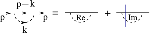
Figure 4: Loop integral contributing to the self energy.

It can be shown that the K-matrix formulation for the T-matrix corresponds to including only the imaginary (or cut-loop) contributions of a certain class of loop diagrams. This guarantees (as was shown before) that unitarity is obeyed. Analyticity of the scattering amplitude is however violated due to ignoring the real contributions of these loop integrals. As a consequence causality will be violated!

To (partially) recover analyticity of the scattering amplitude the so-called “Dressed K-matrix approach”Kon01b has been developed. It is described in the following section.

IV The Dressed K-matrix Model

As discussed in the previous section, the coupled channels K-matrix approach is quite successful in reproducing Compton scattering. However it fails in predicting nucleon polarizabilities. The reason is that, in spite of the many symmetry properties that are satisfied, analyticity or causality of the amplitude is badly violated. In the “Dressed K-matrix” approach the constraint of analyticity is incorporated in an approximate manner without spoiling the other symmetries. In fact analyticity is used as a kind of expansion parameter where presently only the leading contributions are included. The ingredients of the Dressed K-Matrix Model were described in Refs. Kon99 ; Kon00 ; Kon01a and the main results were presented in Ref. Kon01b . The essence of this approach lies in the use of dressed vertices and propagators in the kernel $K$.

The objective of dressing the vertices and propagators is solely to improve on the analytic properties of the amplitude. The imaginary parts of the amplitude are generated through the K-matrix formalism (as imposed by unitarity) and correspond to cut loop corrections where the intermediate particles are taken on their mass shell. The real parts have to follow from applying dispersion relations to the imaginary parts. We incorporate these real parts as real vertex and self-energy functions. Investigating this in detail (for a more extensive discussion we refer to  Kon99 ) shows that the dressing can be formulated in terms of coupled equations, schematically shown in Fig. (5), which generate multiple overlapping loop corrections. The coupled nature of the equations is necessary to obey simultaneously unitarity and analyticity at the level of vertices and propagators.

Figure 5: Graphical representation of the equation for the dressed irreducible $\pi NN$ vertex, denoted by an open circle, and the dressed nucleon propagator, denoted by a solid line. The dashed lines denote pions, the double lines denote $\Delta$s and the zigzag and dotted lines are $\rho$ and $\sigma$ mesons, respectively. The resonance propagators are dressed. The last term in the second equation denotes the counter-term contribution to the nucleon propagator, necessary for the renormalization.

The equations presented in Fig. (5) are solved by iteration where every iteration step proceeds as follows. The imaginary – or pole – contributions of the loop integrals for both the propagators and the vertices are obtained by applying cutting rules. Since the outgoing nucleon and the pion are on-shell, the only kinematically allowed cuts are those shown in Fig. (5). The principal-value part of the vertex (i.e. the real parts of the form factors) and self-energy functions are calculated at every iteration step by applying dispersion relations to the imaginary parts just calculated, where only the physical one-pion–one-nucleon cut on the real axis in the complex $p^{2}$-plane is considered. These real functions are used to calculate the pole contribution for the next iteration step. This procedure is repeated to obtain a converged solution. We consider irreducible vertices, which means that the external propagators are not included in the dressing of the vertices.

Bare $\pi NN$ form factors have been introduced in the dressing procedure to regularize the dispersion integrals. The bare form factor reflects physics at energy scales beyond those of the included mesons and which has been left out of the dressing procedure. One thus expects a large width for this factor, as is indeed the case.

The dressed nucleon propagator is renormalized (through a wave function renormalization factor $Z$ and a bare mass $m_{0}$) to have a pole with a unit residue at the physical mass. The nucleon self-energy is expressed in terms of self-energy functions $A(p^{2})$ and $B(p^{2})$ as $\Sigma_{N}(p)=A_{N}(p^{2})\;/p+B_{N}(p^{2})\;m$.

The procedure of obtaining the $\gamma NN$ vertex Kon00 is in principle the same as for the $\pi NN$ vertex. Contact $\gamma\pi NN$ and $\gamma\gamma NN$ vertices, necessary for gauge invariance of the model, are constructed by minimal substitution in the dressed $\pi NN$ vertex and nucleon propagator, as was explained in Kon00 .

The present procedure restores analyticity at the level of one-particle reducible diagrams in the T-matrix. In general, violation due to two- and more-particle reducible diagrams can be regarded as higher order corrections. An important exception to this general rule is formed by, for example, diagrams where both photons couple to the same intermediate pion in a loop (so-called “handbag” diagrams). This term is exceptional since at the pion threshold the S-wave contribution is large, due to the non-zero value of the $E_{0+}^{1/2}$ multipole in pion-photoproduction, leading to a sharp near-threshold energy dependence of the related $f_{EE}^{1-}$ Compton amplitudeBer93 . In the K-matrix formalism, the imaginary (pole) contribution of this type of diagrams is taken into account. Not including the real part of such a large contribution would entail a significant violation of analyticity. To correct for this, the $\gamma\gamma NN$ vertex also contains the (purely transverse) “cusp” contact term whose construction is described in Section 4 of Ref. Kon00 . Since, due to chiral symmetry, the S-wave pion scattering amplitude vanishes at threshold, the mechanism that gives rise to the important “cusp” term in compton scattering does not contribute to $\pi\pi NN$ or $\pi\gamma NN$ contact terms. The analogons to the “cusp” $\gamma\gamma NN$ term will thus be negligible and have therefore not been considered.

IV.1 Results

Results for pion-nucleon scattering and pion-photoproduction obtained in the dressed K-matrix model and in the traditional K-matrix approach are of comparable quality. One should, however, expect the two approaches to have significant differences for Compton scattering since for this case constraints imposed by analyticity will be most important Pfe74 ; Ber93 .

The effect of the dressing on the $f_{EE}^{1-}$ amplitude can be seen in Fig. (6), where also the results of dispersion analyses are quoted for comparison. Note that the imaginary parts of $f_{EE}^{1-}$ from calculations B (Bare, corresponding to the usual K-matrix approach) and D (Dressed, the full Dressed K-matrix results) are rather similar in the vicinity of threshold.

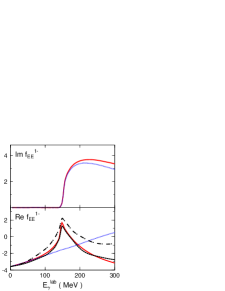
Figure 6: The $f_{EE}^{1-}$ partial amplitude of Compton scattering on the proton in units $10^{-4}/m_{\pi}$. Solid line: dressed K-matrix, D; dotted line: bare K-matrix, B. Also shown are the results of the dispersion analyses of Ref. Pfe74 (dash-dots) and Ref. Ber93 (dashed).

The polarizabilities characterize response of the nucleon to an externally applied electromagnetic field Hem98 ; Hol00 . They can be defined as coefficients in a low-energy expansion of the cross section or partial amplitudes of Compton scattering. Since gauge invariance, unitarity, crossing and CPT symmetries are fulfilled in both models the Thompson limit at vanishing photon energy is reproduced. Our results for the electric, magnetic and spin polarizabilities of the proton are given in Table 1, where they are compared with the results given in refs. Hem98 ; Gel00 and with the values extracted from recent experiments. The contribution from the the t-channel $\pi^{0}$-exchange diagram has been subtracted. The effect of the dressing on the polarizabilities can be seen by comparing the values given in columns D (dressed) and B (bare). In particular, the dressing tends to decrease $\alpha$ while increasing $\beta$. Among the spin polarizabilities, $\gamma_{E1}$ is affected much more than the other $\gamma$’s. The effect of the additional “cusp” $\gamma\gamma NN$ contact termKon00 , strongly influences the electric polarizabilities rather than the magnetic ones. This is because the “cusp” contact term affects primarily the electric partial amplitude $f_{EE}^{1-}$ (corresponding to the the total angular momentum and parity of the intermediate state $J^{\pi}=1/2^{-}$) rather than the magnetic amplitude $f_{MM}^{1-}$ ($J^{\pi}=1/2^{+}$).

Table 1: Polarizabilities of the proton. The units are $10^{-4}fm^{3}$ for $\alpha$ and $\beta$ and $10^{-4}fm^{4}$ for the $\gamma$’s (the anomalous $\pi^{0}$ contribution is subtracted). The first two columns contain the polarizabilities obtained from the present calculation; D (full, dressed) and B (bare K-matrix). The two columns named $\chi PT$ contain the polarizabilities calculated in the chiral perturbation theory Hem98 ; Gel00 . Results of recent dispersion analyses are given in the last column (Ref. Lvo97 for $\alpha$ and $\beta$ and Ref. Dre00 for the $\gamma$’s).

			$\chi_{PT}$		DA
	D	B	Gel00	Hem98
$\alpha$	12.1	15.5	10.5	16.4	11.9
$\beta$	2.4	1.7	3.5	9.1	1.9
$\gamma_{E1}$	-5.0	-1.7	-1.9	-5.4	-4.3
$\gamma_{M1}$	3.4	3.8	0.4	1.4	2.9
$\gamma_{E2}$	1.1	1.0	1.9	1.0	2.2
$\gamma_{M2}$	-1.8	-2.3	0.7	1.0	0.0
$\gamma_{0}$	2.4	-0.9	-1.1	2.0	-0.8
$\gamma_{\pi}$	11.4	8.9	3.5	6.8	9.4

Of special interest is to check whether polarizabilities as extracted form the low energy behavior of the amplitude are in agreement with the values as extracted from energy weighted sumrules. The derivation of sumrules is based on the fact that the amplitudes obey certain symmetries where analyticity is of particular importance. This comparison is still in progess and results will be published in a forthcoming paper Kon01c . Preliminary results indicate that the different sum rules are obeyed, with the exception of the sum rule for the spin polarizability $\gamma_{0}$. This may be due to an incomplete dressing of the $\Delta$-resonance in the present calculational scheme.

V Summary and Conclusions

Results are presented for Compton scattering on a free proton as well as on a nucleus. For processes on the proton the usual K-matrix model as well as the recently developed dressed K-matrix model are discussed. In the latter approach the real self energies and vertex functions are obtained from the imaginary parts using dispersion relations imposing self-consistency conditions. It is indicated that such an approach is essential to understand features seen in the data, in particular at energies around and below the pion production threshold.

References

- (1) P. F. A. Goudsmit, H. J. Leisi, E. Matsinos, B. L. Birbrair, and A. B. Gridnev, Nucl. Phys. A 575, 673 (1994).
- (2) O. Scholten, A.Yu. Korchin, V. Pascalutsa, and D. Van Neck, Phys. Lett. B 384, 13 (1996).
- (3) T. Feuster and U. Mosel, Phys. Rev. C 58, 457 (1998); ibid, Phys. Rev. C 59, 460 (1999).
- (4) A. Yu. Korchin, O. Scholten, and R.G.E. Timmermans, Phys. Lett. B 438, 1 (1998).
- (5) V. Pascalutsa, Phys. Lett. B 503, 85 (2001).
- (6) S. Kondratyuk and O. Scholten, Phys. Rev. C 59, 1070 (1999); ibid, Phys. Rev. C 62, 025203 (2000).
- (7) S. Kondratyuk and O. Scholten, Nucl. Phys. A 677, 396 (2000).
- (8) S. Kondratyuk and O. Scholten, Nucl. Phys. A 680, 175c (2001).
- (9) S. Kondratyuk and O. Scholten, Phys. Rev. C 64, 024005 (2001).
- (10) S. Kondratyuk and O. Scholten, nucl-th/0109038.
- (11) E.L. Hallin et al., Phys. Rev. C 48, 1497 (1993).
- (12) W. Pfeil, H. Rollnik, and S. Stankowski, Nucl. Phys. B 73, 166 (1974).
- (13) J.C. Bergstrom and E.L. Hallin, Phys. Rev. C 48, 1508 (1993).
- (14) T.R. Hemmert, B.R. Holstein, and J. Kambor, Phys. Rev. D 57, 5746 (1998).
- (15) B.R. Holstein, hep-ph/0010129.
- (16) G.C. Gellas, T.R. Hemmert, and Ulf-G. Meissner, Phys. Rev. Lett. 85, 14 (2000).
- (17) A.I. L’vov, V.A. Petrun’kin, and M. Schumacher, Phys. Rev. C 55, 359 (1997).
- (18) D. Drechsel, M. Gorchtein, B. Pasquini, and M. Vanderhaeghen, Phys. Rev. C 61, 015204 (2000).