Classical Drop Phase Diagram and Cluster Distributions

Abstract

The phase diagram, ($T,\rho$), of a finite, constrained, and classical system is built from the analysis of cluster distributions in phase and configurational space. The obtained phase diagram can be split in three regions. One, low density limit, in which first order phase transition features can be observed. Another one, corresponding to the high density regime, in which fragments in phase space display critical behavior of 3D-Ising universality class type. And an intermediate density region, in which power-laws are displayed but can not be associated to the abovementioned universality class.

PACS number(s): 25.70 -z, 25.70.Mn, 25.70.Pq, 02.70.Ns

I Introduction

The multifragmentation phenomenon that takes place in nuclei with excitation energies above 2 MeV/nucleon has been one of the central issues of the nuclear community during the past two decades. Many experimental and theoretical efforts have been concentrated towards the understanding of the mechanisms involved in that process. In particular, one feature that triggered the interest on the field was the important detected production of intermediate mass fragments (IMF’s). Highly excited nuclei break up in many IMF’s in Fermi energy range reactions. This feature, along with the fact that early calculations of caloric curves showed an approximately constant behavior, was interpreted by many groups as a signature of a phase transition taking place in finite nuclear systems [1, 2, 3, 4]. In recent contributions the behavior of the microcanonical heat capacity was used to experimentally characterize the transition as a first order one [6]. Within this picture, the latent heat can be associated with the transformation between a Fermi liquid and a gas phase, composed by light particles and free nucleons.

Despite that the familiar liquid-gas transition framework seems to be appropriate to deal with the nuclear case, there are some peculiarities that are worth to be considered. One key point usually disregarded is that, by its own nature, multifragmentation in nuclear reactions should be a priori analyzed as a nonequilibrium process (see [7, 8]). Even if an equilibrium scenario is adopted, a major point is that we are dealing with a phase transition occurring in a finite system. Therefore, several thermodynamical features, e. g. the entropy extensivity, cannot be taken for granted and the agreement between different statistical ensembles predictions cannot be invoked anymore [10]. A working hypothesis, usually made by statistical models in order to apply a tractable global equilibrium picture, is that a freeze-out volume can be defined inside of which the existence of an equilibrated ensemble of clusters can be assumed. In these models, the behavior of thermodynamics quantities is closely related to the way the system is partitionated into clusters giving rise to internal surfaces (isolated drops).

The aim of the present paper is to analyze the relationship between cluster distributions inside a fixed volume and the respective thermodynamic description. In order to do that a confined system that interacts via a two-body Lennard-Jones potential is studied. A molecular dynamics, MD, approach is used. The analogy between the nuclear force and the van der Waals interaction supports the use of this simplified classical model to obtain qualitatively meaningful results.

Given the MD microcanonical description, a connection with thermodynamical quantities can be established via well known principles from mechanics. For instance, the pressure and temperature can be estimated from the generalized equipartition theorem [11], whereas the specific heat can be related to kinetic energy fluctuations [12]. On the other hand, a complementary analysis of the microscopic correlations at a “nucleon” level of description can also be considered. To that end, different fragment-recognition algorithms can be used in order to unveil different particle correlation properties.

Previous studies [13] have already dealt with this ’cluster structure-thermodynamic description’ mapping. They made used of a cluster definition à la Coniglio-Klein, and were mainly focused on the system behavior in the supercritical phase ($\rho>\rho_{c},T>T_{c}$).

In this contribution we consider two alternative fragment definitions that, differently from Coniglio-Klein clusters (that in the present paper will be called MSTE clusters, as will be explained in Sec. III), are built in well defined and physically meaningful spaces. The first one, associated with the so called minimum spanning tree fragment recognition method, is based on configurational information (MST clusters)[14]. The second one uses complete phase space information in order to define a fragment set according to the most bound density fluctuation in phase space [16] (ECRA clusters). Using this fragment characterization as a fundamental piece of information, consistent phase diagrams are built from scratch for the analyzed finite systems. In addition, the relationship between critical signatures in the fragment distributions and the corresponding system localization in the phase diagram is established.

This paper is organized as follows. In Section II we will describe the model used in our simulations. Section III is devoted to a characterization of the used cluster definitions. A description of expected signals associated with phase transitions in finite systems is given in Section IV. In Section V the study of phase diagram is presented. Finally, in Section VI, conclusions are drawn.

II The model

The system under study is composed by excited drops made up of particles interacting via a 6-12 Lennard Jones potential, which reads:

$$V(r)=\left\{\begin{array}[]{ll}4\epsilon\left[\left(\frac{\sigma}{r}\right)^{12}-\left(\frac{\sigma}{r}\right)^{6}-\left(\frac{\sigma}{r_{c}}\right)^{12}+\left(\frac{\sigma}{r_{c}}\right)^{6}\right]r\leq r_{c}&\\ 0r$>$r_{c}&\end{array}\right.$$ (1)

We took the cut-off radius as $r_{c}=3\sigma$. Energies and distances are measured in units of the potential well ($\epsilon$) and the distance at which the potential changes sign ($\sigma$), respectively while the unit of time used is: $t_{0}=\sqrt{\sigma^{2}m/48\epsilon}$.

In order to constrain the dynamics we used a spherical confining ‘wall’. The considered external potential behaves like $V_{wall}\sim(r-r_{wall})^{-12}$ with a cut off distance $r_{cut}=1\sigma$ , where it smoothly became zero along with its first derivative. The set of classical equations of motion were integrated using the well known velocity Verlet algorithm [17], taking $t_{int}=0.002t_{0}$ as the integration time step. Once the transient behavior was over a microcanonical sampling of particle configurations every $5t_{0}$ up to a final time of $140000t_{0}$ was performed.

III Fragment Definitions

The simplest and more intuitive cluster definition is based on correlations in configuration space: a particle $i$ belongs to a cluster $C$ if there is another particle $j$ that belongs to $C$ and $|{\bf r_{i}}-{\bf r_{j}}|\leq r_{cl}$, where $r_{cl}$ is a parameter called the clusterization radius.

We set $r_{cl}=r_{c}=3\sigma$. The algorithm that recognizes these clusters is known as “Minimum Spanning Tree” (MST). In this method only correlations in q-space are used, neglecting completely the effect of momentum. As was shown in Ref. [14], MST clusters give incorrect information about the meaningful fragment structure of the system for dense configurations. However, an interesting point to be notice is that it can still provide useful information about the limit imposed by the constraining finite volume to the formation of well defined fragments in configurational space. As $r_{cl}=r_{cut}$, no inter-cluster interaction exists, so cluster surfaces can be univocally defined.

An extension of the MST is the “Minimum Spanning Tree in Energy” space (MSTE) algorithm. In this case, a given set of particles $i,j,...,k$, belongs to the same cluster $C_{i}$ if:

$$\forall\,i\,\epsilon\,C_{i}\>,\>\exists\,j\,\epsilon\,C_{i}\,/\,e_{ij}\leq 0$$ (2)

where $e_{ij}=V(r_{ij})+({\bf p}_{i}-{\bf p}_{j})^{2}/4\mu$, and $\mu$ is the reduced mass of the pair $\{i,j\}$. This cluster definition resembles the clusterization prescription adopted by Coniglio and Klein [18] and was the one used by Campi et al. in Ref.[13]. The MSTE algorithm searches for configurational correlations between particles considering the relative momenta of particle pairs, and typically recognizes fragments earlier than MST in highly excited unconstrained systems[14, 15].

Finally, a more robust cluster definition is based on the system “most bound density fluctuation”(MBDF) in phase space [16]. The MBDF is composed by the set of clusters $\{C_{i}\}$ for which the sum, $E_{\{C_{i}\}}$, of the fragment internal energies attains its minimum value:

$$E_{\{C_{i}\}} = \sum_{i}E_{int}^{C_{i}}$$ (3)

$$\mbox{with }E_{int}^{C_{i}} = \sum_{j\in C_{i}}K_{j}^{cm}+\sum_{{j,k\in C_{i}}\atop j\leq k}V_{j,k}$$ (4)

$K_{j}^{cm}$ is the kinetic energy of particle $j$ measured in the center of mass frame of the cluster which contains particle $j$, and $V_{ij}$ stands for the inter-particle potential.

The algorithm that finds the MBDF is known as the “Early Cluster Recognition Algorithm” (ECRA). It searches for simultaneously well correlated structures in both, q, and p space, via the minimization of the potential and the kinetic terms respectively.

The ECRA algorithm has been used extensively in many studies of free expanding fragmenting systems  [7, 19] and has helped to discover that excited drops break very early in the evolution. In addition, in a recent contribution [8] it was shown that ECRA clusters are also suitable to describe the fragmentation transition that takes place in volume constrained systems.

IV Characterizing the transition

As mentioned in the introduction, several observables can be studied in order to analyze phase transitions phenomena occurring in finite systems. They usually involve the behavior of caloric curves [2, 3, 20, 21, 22, 23], specific heats [6, 24], kinetic energy fluctuations [4, 5], fragment mass distributions [25, 26], and critical exponents [26].

A Thermodynamical Description

One of the most relevant quantities in the study of fragmenting systems, either constrained or free to expand is the caloric curve (CC). The CC is defined as the functional relationship between the system energy and its temperature, given by:

$$T(E)={2\over{3(N-1)}}<K>_{E}$$ (5)

being N the number of particles, and $<K>_{E}$ the mean kinetic energy averaged over a fixed total energy MD simulation [9].

In Figure 1(a) the CC’s are shown for the following densities: $\rho^{h}=0.55\sigma^{-3},\rho^{c}=0.35\sigma^{-3},\rho^{m}=0.07\sigma^{-3},$ and $\rho^{l}=0.01\sigma^{-3}$.

FIG. 1.: The caloric curve is shown in panel (a). In panels (b) and (c) the potential energy ($V$) and its root mean squared deviation as a function of the system total energy are displayed in panels (b) and (c) respectively. The following density values: $\rho=0.01,0.07,0.35,$ and $0.55\sigma^{-3}$, displayed with full triangles, diamonds, squares, and circles respectively, were considered.

Different behaviors can be recognized. For the more diluted case, $\rho^{l}$ (full triangles), the corresponding CC displays a loop which ends in a linearly increasing temperature line, which we refer as vapor branch. Taking into account that, within the microcanonical ensemble, the specific heat is defined as:

$${1\over{C}}=\frac{\partial T}{\partial E}=-T^{2}\frac{\partial^{2}S}{\partial E^{2}}$$ (6)

it is clear that for this case negative values of $C$ will be found in the range $0.1\epsilon_{0}<E<0.6\epsilon_{0}$. A negative value of the derivative of the temperature as a function of the energy reflects an ’anomalous’ behavior of the system entropy for the respective energy range. A convex intruder in $S(E)$, prohibited in the thermodynamical limit, arises as a consequence of the finiteness of the system and the corresponding lack of extensivity of thermodynamical quantities like $S$. This signal is expected in first order phase transitions, and is associated to a negative branch of the heat capacity between two poles [10]. Taking into account the relationship between kinetic energy fluctuations and the system specific heat [5, 29]:

$${1\over N}<(\delta K)^{2}>_{E}={3\over{2\beta^{2}}}(1-{3\over{2C}})$$ (7)

it can be seen that negative values of the specific heat appear whenever $(\delta K)^{2}$ get larger than the canonical expectation: ${3N\over{2\beta^{2}}}$. This behavior has already been verified in Ref.[8].

As the density is increased the loop is washed away and it is replaced by an inflection point ($\rho^{m}$, full diamonds in Fig.1(a)). This corresponds to the merging of the specific heat negative poles into a single local maximum. Finally, for higher densities, $\rho^{c}$ and $\rho^{h}$ (filled diamonds, and circles), no major changes in the CC’s second derivative is observed.

In Fig. 1(b) the mean potential energy per particle, $V$, as a function of the total system energy is displayed. For the lowest densities two different regimes can be recognized. First, a steep increasing behavior for energies $E<0.5\epsilon_{0}$, that can be related to an increase of the mean interparticle distance and the appearance of internal surfaces, as the number of atractive bonds decreases. Second, a saturating behavior for larger energy values, $E>0.5\epsilon_{0}$. For more dense systems, no such feature can be observed. A smooth behavior is displayed by $V$.

Another interesting feature can be noticed looking at the root mean square deviation of partial energies (kinetic or potential), $\sigma_{V,K}$, shown in Fig. 1(c). For the lowest densities (filled triangles and diamonds) an abrupt decrease is observed at $E\sim 0.5\epsilon_{0}$, whereas for the highest considered density, $\rho^{h}=0.8\sigma^{-3}$(filled circles), no trace of such behavior can be reported. For future reference, it is worth noting that the transition in the monotonic character of the curve takes place at a density value $\rho\sim\rho^{c}=0.35\epsilon_{0}$(filled squares).

To attain a better understanding of the behavior of the magnitudes displayed in Figs. 1(b), and (c), we have followed two strategies: i) to study particle-particle correlations, ii) to analyze fragment mass distributions according to the already presented fragment definitions. In what follows we present results obtained within the first approach, and postpone to the next subsection the analysis of fragment properties.

In Fig.2 the distribution of interparticle distances, $r_{ij}$, is shown. Two density values already considered in Fig1, namely $\rho^{h}$ and $\rho^{l}$, are shown in panels (a) and (b) respectively.

For each density, three total energy values, lower than(solid line), equal to (dotted line), and larger than (dashed line) $E=0.5\epsilon_{0}$, were considered (see caption). In both panels, a vertical line was included indicating the interaction cut-off radius.

FIG. 2.: Normalized interparticle distance distribution calculated for $\rho^{l}$ and $\rho^{h}$ systems are shown in panels (a) and (b) respectively. The following three total energy values, $E=0.0,0.5,1.0\epsilon_{0}$, were considered in panel (a), whereas $E=-0.50,0.5,1.0\epsilon_{0}$ for panel (b). They are shown with, solid, dotted, and dashed lines respectively. Note the different scales used for $r_{ij}$ in both panels.

In panel (a) (very diluted case) a well defined structure of interacting particle pairs can be seen at low energies (continuous line). The displayed peaks signal the presence of a rather large self-sustained drop, with a first, second and even third nearest neighbors structure. As energy increases, this structure fades away, and an important reduction of the number of interacting particles can be noticed. This occurs as a consequence of the spacious volume available , that is big enough to accommodate small non-overlapping particle aggregates. In this transition, well defined q-space clusters appear, surfaces are produced and $V$ tends towards a residual value (see bellow).

A completely different behavior is observed for the denser instance, $\rho^{h}$, shown in Fig. 2(b). In this case, no changes in the statistical distribution of $r_{ij}$ is observed as the energy is increased. (Note that the bell shaped distribution associated with the ‘trivial’ noninteracting pair counting is superimposed over the peak structure. However, the presence of a first, second, and even a third nearest neighbors can still be traced). The container imposes a severe volume restriction on the system, and even for high total energy values, each particle is confined in the attractive concavity of partners potential, between the repulsive core of nearest neighbors.

This last observation can complete a general picture, within which the behavior of the mean potential energy, $V$, for the high density cases can be easily understood. As more energy is added to the system no structural transition is allowed by the constraining volume. Particles can not escape from neighbors most attractive potential range and a smooth increased in $V$, related to the average time spent in the most negative potential areas, can be seen (Fig 1(b)).

The decreasing of $\sigma_{V}$, observed for low densities (filled triangles, and diamonds in Fig. 1(c)), can be associated to the loss of ‘attractive bonds’ between particle pairs that takes place when a non interacting light cluster regime dominates. As an increasing number of particles stop interacting with one another, the system dynamics gets ’less chaotic’ (see [28] for a dynamical characterization of this system), and a decrease of $\sigma_{V}$ is induced.

On the other hand, for high densities, the region with the strongest non-lineal nature becomes the most relevant part of the interaction potential. As a consequence of that, an increase of the fluctuations in potential energy between successive configurations as total energy is added can be expected (see the behavior displayed by $\sigma_{V}$ in Fig 1(c)).

It is worth noting that the presented picture can also be used to interpret recent results regarding the behavior of the maximum Lyapunov exponent, MLE, in constrained systems (see [28]). Moreover, a striking similitude between the behavior of $\sigma_{V}(E,\rho)$ and $MLE(E,\rho)$ can be noticed, comparing Fig.1(c), and Fig.5 of Ref. [28].

B Fragments Inside the Volume

In section III, three fragment recognition algorithms were described. Each one of them make use of different correlation information in order to link particles into clusters, and then give different physical information about the system under study.

FIG. 3.: MST cluster mass distributions calculated for densities: $\rho=0.01,0.03$, and $0.10\sigma^{-3}$ are displayed in panels (a), (b), and (c) respectively. Three total energy values were considered for each density, $E_{tot}=0.0,0.5$, and $1.0\epsilon_{0}$.They are displayed as full, dotted and dashed lines respectively

In Fig. 3 the results of the MST algorithm analysis are shown. MST spectra were calculated for different energies ($E=0.0,0.5$, and $1.0\epsilon_{0}$, displayed as full, dotted and dashed lines respectively) for three system densities: $\rho=0.01,0.03$, and $0.10\sigma^{-3}$. They are shown in panels (a), (b), and (c), of Fig.3 respectively.

At low densities, panel 3(a), the system evolves from a heavy cluster dominated behavior at low energies, towards a light cluster dominated behavior, at high energies. This reflects the fact that the constraining volume is large enough to allow the system to fragment in well defined drops as energy is increased. It is interesting to notice that results displayed in Fig. 3(a) correspond to full triangle symbols in Fig.1(a), i.e. the one for which the CC displays a loop. It was argued that big fluctuations in kinetic energy should be expected. This is indeed the case and it is related to the fact that well defined surfaces appear in the system (see [8]).

On the other hand, as density increases, the mass distributions converge to a u-shaped one. Almost no spatially well separated structures (i.e. MST clusters) can be identified, aside from the trivial huge cluster that comprises almost all the system particles.

In Fig. 4, the effect of taking into account momentum correlation in the definition of clusters is displayed. There, a cluster analysis for a system of $N=147$ particles with $\rho=0.2\sigma^{-3}$ using ECRA, MSTE, and MST prescriptions is presented. The mass distribution function, and the fragment internal energy as a function of the cluster mass, $E_{int}(s)$, are shown in the first and second columns, respectively. Three total energy values were considered: $E_{tot}=-0.6$ (panels (a)-(b)), $0.0$ (panels(c)-(d)), and $0.5\epsilon_{0}$ (panels (e)-(f)). Empty triangles, solid squares, and empty circles correspond to MST, MSTE, and ECRA results respectively.

FIG. 4.: Fragment mass distribution, and cluster internal energy values as a function of the cluster mass, are shown in the first and second columns respectively. Three system total energies are considered: $E_{tot}=-0.6\epsilon_{0}$, panels (a-b), $0.0\epsilon_{0}$, panels (c-d), and $0.5\epsilon_{0}$, panels (e-f). Empty circles, filled squares, and empty triangles, correspond to ECRA, MSTE, and MST data, respectively.

It can be seen that, for this density, the MST prescription finds just a big drop. On the other hand, both, the MSTE and ECRA algorithms, find non-trivial cluster distributions that show the expected transition from a u-shaped, towards and exponential behavior, as the system energy is increased. As a general rule, ECRA algorithm produces more bound clusters than the MSTE one. This is consistent with the claim that the MBDF are found by the ECRA algorithm. Due to this feature, from now on, just the properties of the system according to its ECRA cluster structure will be considered.

C Transition Signals

As seen in Fig.4, in which a system at a $\rho=0.2\sigma^{-3}$ density was considered, the ECRA cluster distributions undergo a transition from a U-shaped spectrum towards an exponentially decaying one. Moreover, the one corresponding to the intermediate energy value 4(b), displays a power law like behavior. In fact, for any other density studied, the same behavior can be reported, and a total energy value can be determined, for which a power-law like mass distribution can be found.

This result is interesting, because it implies that some kind of transition between two regimes, one with, and other without large ECRA drops, i.e. with or without the presence of liquid-like structures, is taking place in high density systems. Moreover, this transition can not be detected simply using spatial correlations information. In this way, considering the appropriate cluster prescription, power-law mass distributions can be used to trace the transition line in a $(T,\rho)$ diagram.

Within the Fisher Droplet Model [34], when dealing with infinite systems, one expects to find such a scale-free distribution at a critical point, where a continuous transition takes place, and scaling hypothesis can be applied. However, it has been reported [23, 30, 31] that several critical signatures also appear when first order phase transition are analyzed in small systems. In particular, as stated in Ref [31], in small systems the largest cluster gets a size comparable to the vapor fraction before dissapearing when the system crosses the coexistence line. Therefore there is an energy for which a pseudo-invariance of scale and a resemblance with critical behavior can be expected for small systems undergoing phase transitions that, in the thermodynamical limit, would be univocally classified as first order ones.

In order to search for a power-law behavior in fragment distributions the following single parameter function was employed to fit fragment mass spectra. The contribution of the largest fragment was disregarded [26]:

$$n(A)=q_{0}A^{-\tau}\mbox{ ,with }q_{0}(\tau)=\frac{1}{\sum_{A}A^{1-\tau}}$$ (8)

$n(A)$ is the number of fragments with mass number $A$, and $q_{0}$ is a normalization constant.

The quality of the fitting procedure was quantified using the standard $\chi^{2}$ coefficient (see [32] for details), and an energy value, $E_{*}$, was associated to the best fitted spectra. In Fig.5(a) a typical $\chi^{2}$ calculation is shown for ECRA clusters in a $\rho=0.10\sigma^{-3}$ system. From the figure, a value of $E_{*}=0.10\pm 0.05\epsilon_{0}$, can be reported.

FIG. 5.: Transition signatures calculated for a $\rho=0.10\sigma^{-3}$ system. The $\chi^{2}$ fitting coefficient, the second moment of the mass distribution, $M_{2}$, and the normalized mean variance of the largest fragment, NVM, are displayed in panels (a), (b), and (c) respectively.

Another useful observable to search for scale-free distribution functions is the second moment of the cluster distribution $M_{2}=\sum^{\prime}_{A}A^{2}n(A)$. As in the determination of $\tau$, the largest cluster is excluded from the primed sum. $M_{2}$ is proportional to the compressibility $\kappa_{T}$, that, in the thermodynamical limit, presents a power-law singularity at a second order transition. For finite system the divergence is replaced by a maximum. In panel 5(b) it is shown the estimation of $M_{2}(E)$, for a $\rho=0.10\sigma^{-3}$ system. It can be noticed that the maximum is located at the energy value for which the spectra is best fitted by a power-law like dependence.

This kind of agreement is also achieved when the normalized mean variance, NVM, of the largest fragment mass, $A_{max}$, is analyzed. NVM is defined as:

$${\mbox{N}VM}=\frac{<A_{max}^{2}>-<A_{max}>^{2}}{<A_{max}>}$$ (9)

and it proved to be a robust tool for the characterization of transition phenomena in which an enhancement of fluctuations occurs[33]. As can be seen from panel 5(c), this signal, although slightly shifted within the working resolution, also peaks in the same region of the previous ones.

The signal agreement reported for the $\rho=0.10\sigma^{-3}$ case in Fig.5, is also achieved for every density analyzed in this paper. This means that, in the whole density range, power-law mass distributions for phase space defined ECRA clusters are found whenever large fluctuations take place in the system.

In order to properly characterize the state of the system which displays power-law mass distributions, the values attained by the $\tau$ exponents must be analyzed, as a function of the density. This dependence is shown in Fig.6(a). For a true critical phenomenon, taking place in three dimensional systems, $2\leq\tau\leq 3$ is expected [34]. This condition is not satisfied for systems with $\rho<0.05\sigma^{-3}$. For this highly diluted systems, the observed free-scale distribution is not expected to survive the thermodynamic limit. It is not related to any continuous transition, but arises as a finite-size effect. It is worth noting that $\rho\sim 0.05\sigma^{-3}$ is the maximum density for which the respective caloric curve displays a loop, and then, negative $c_{v}$ (see Fig.1).

FIG. 6.: Estimated values from ECRA cluster distributions for the critical exponents $\tau$ and $\gamma$ are shown in panels (a), and (b) respectively. The expected values for the 3D-Ising universality class are displayed by a dashed line.

On the other hand, for $\rho>0.05$, the calculated $\tau$ exponents show a rather good agreement with the $\tau=2.21$ value (dashed line), expected for liquid-gas transitions.

In a second order phase transition, the behavior of $M_{2}$ near a critical point can be described in terms of the critical exponent $\gamma$ [26]:

$$M_{2}(\epsilon)\propto|\epsilon|^{-\gamma}.$$ (10)

where, $\epsilon=(Ec-E)/E_{c}$, measures the distance to the critical point. This relation is valid for an infinite system in the limit $\epsilon\rightarrow 0$. As already mentioned, in a finite system $M_{2}$ displays a maximum instead of the divergence predicted in equation (10). Having this in mind, a calculation procedure introduced in Ref.[27] ($\gamma$-matching), that takes care of finite size effects, was used to calculate the $\gamma$ exponent value for our system (see also Ref.[32] for details).

The results of the $\gamma$ exponent estimation is shown in Fig.6(b). The obtained values tends toward $\gamma_{liq-gas}=1.23$ (dashed line) value, that is expected for a liquid-gas transition. It is worth noting that this convergence is achieved for densities $\rho\geq 0.35\epsilon_{0}$ (this value equals $\rho^{c}$ in Fig.1). For this density, a change in the behavior of the potential energy fluctuations as a function of the total energy was reported in Fig.1(c). This can be associated (see Sec.IV A) to the onset of the invariance of the statistical interparticle distance distribution (Fig.2), that takes place as a consequence of the imposed volume restriction, and precludes the occurrence of a continuous transition.

V Phase Diagram

In the previous section several signatures of a change in the properties of ECRA fragment mass distributions were analyzed. At any given density, a system energy, $E_{*}(\rho)$, can be determined for which large fluctuations appear in the system, and a scale-free like mass distribution can be found.

FIG. 7.: Density dependence of the system energy, $E_{*}$, at which transition signals are detected. The dashed line is included to guide the eye.

In Fig.7, the dependence of $E_{*}$ with the system density can be seen. It can be noticed that for $\rho\geq 0.35\sigma^{-3}$, a rather constant value is attained for the transition energy. A similar result was reported in Ref.[13], using the already presented MSTE cluster definition.

Some insight about the properties of the system along the line depicted in Fig.7, can be gained from the analysis of the interplay between the mean internal potential energy per particle stored in ECRA clusters, $V_{int}$, and the mean inter-cluster interaction energy, $V_{ic}$.

$$V_{int} = \sum_{i<j\atop{i,j\in C_{k}}}V_{i,j}$$ (11)

$$V_{ic} = \sum_{{{i\in C_{k}}\atop{j\in C_{l}}}\atop k\neq l}V_{i,j}$$ (12)

$V_{int}$ stands for the mean potential felt by a particle in a cluster due to its interaction with the other members of the same cluster. On the other hand, $V_{ic}$ represents the mean interaction potential felt by a particle due to its interactions with particles belonging to the other clusters. This magnitudes are displayed in Fig.8 for densities $\rho=0.01,0.20,0.50$, and $0.80\sigma^{-3}$ in panels (a) to (d) respectively.

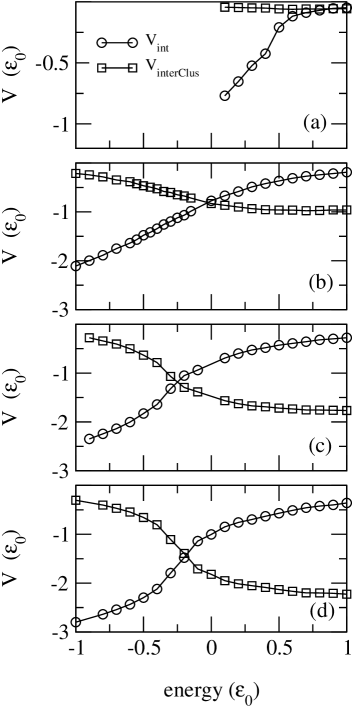
FIG. 8.: $V_{int}$ (empty circles) and $V_{ic}$ (empty squares) as a function of the system total energy are shown. Densities: $\rho=0.01,0.20,0.50$, and $0.80\sigma^{-3}$ are displayed in panels (a), (b), (c), and (d), respectively

The general trend displayed by $V_{int}$ and $V_{ic}$ is easy to understand. At any given density, for low energies, a big ECRA cluster can be found having a large binding energy. In addition, as no many other clusters beside the biggest one exist, $V_{ic}\sim 0$. At high energies, the ECRA partitions turn out to present a rather high multiplicity of light clusters. Consequently $V_{int}\rightarrow 0$ in this limit and $V_{ic}$ absolute value increases.

After a close inspection of Fig.8, one can realize that, for any given density, the energy at which $V_{int}=V_{ic}$, happens to be $E_{*}(\rho)$, i.e. the energy at which power-law like mass distributions appear. This means that scale-free ECRA mass distributions have the following property: a balance is established between the mean potential energy a particle, that belongs to a given cluster, feels due to its interaction with other members of the same cluster and the one associated with its interaction with the rest of the particles in the system. This potential energy balance, that does not allow to distinguish contributions from inside or outside of a cluster, is reminiscent of the vanishment of the chemical potential and surface tension terms that takes place at the critical point within the Fisher droplet model framework [34].

Gathering all the information obtained so far, the phase diagram for our 147-particle Lennard-Jones drop can be built. In Fig.9 the resulting phase diagram is presented. The empty circles are $(T_{*},\rho)$ points obtained from the aforementioned cluster analysis. The full line is an estimation of the coexistence line, as obtained from the analysis of the system specific heat, $c_{v}$ (see Eq.7). In this case, for densities for which the respective CC displays a loop, $T(E_{*})$ has been taken as the average temperature between the two values corresponding to the location of the $c_{v}$ singularities. For denser cases, the location of the maximum of the $c_{v}$ has been taken. No reliable estimation of the energy that maximizes $c_{v}$ could be achieved for $\rho>0.35\sigma^{-3}$.

FIG. 9.: Phase diagram for a 147 particle Lennard Jones drop. Cluster-based and $c_{v}$-based determination of the coexistence line is marked with empty circles, and full line respectively. The dashed line is included to guide the eye.

From the figure, it can be seen that the symmetry between low and high densities, characteristic for the infinite size limit, is lost in the finite size system. An almost linear raising branch, for $\rho>\rho^{c}$, can be seen instead. For every density value, below the depicted coexistence line, a liquid-like ECRA structure can be identified, whereas a vapor behavior can be observed above it.

It is interesting to notice that three density regions can be identified. The region labelled $A$ ($\rho\leq 0.05\sigma^{-3}$) presents the signals expected for a first order phase transition occurring in a finite system: the corresponding caloric curve shows a loop that can be associated to a negative specific heat, and a structural transition can be recognized (Fig.2(a)). These region is the only one in which the available volume is large enough for the system to fragment into a set of non-overlapping drops.

On the other hand, in region $C$ ($\rho>0.35\sigma^{-3}$), where the system is rather compressed, and MST algorithm recognizes just one big fragment, a second order transition seems to occur in phase space, whenever the transition line is crossed. No anomaly in the respective caloric curve is observed, no qualitative changes in the configuration statistical properties is reported (Fig.2(b)), and the calculated critical exponents, $\tau$, and $\gamma$, are in good agreement with 3D-Ising (liquid-gas) universality class.

In between those two regions, region $B$ ($0.05\sigma^{-3}<\rho<0.35\sigma^{-3}$) can be identified. The finite size of the system plays a major role in this density range. Even a sensible $\tau$ value suggests that physically meaningfull scaling properties are present in the system, the corresponding $\gamma$ exponent values are too low to classify the transition as a continuous one.

VI Conclusions

In this paper we have undertaken the analysis of thermodynamical properties of a finite classical system confined in a volume. Apart from the basic interest on such a problem, it might be relevant on the frame of the description of fragmenting system according to statistical models.

We have been able to find, that from a coordinate space stand point the equation of state of such a system is quite simple. There is a maximum value of the density ($\rho\sim 0.05\sigma^{-3}$) up to which the system can undergo a first order phase transition. In this region, the associated CC displays a loop and the thermal response function attains negative values. This feature allowed us to define a transition curve. For higher densities, there is simply no room enough to allow the system to develop well defined internal surfaces, i.e. only one big drop can be detected.

When one turns into a description of fragments in which correlations in p-space are taken into account, a much reacher structure appears. Now, even for densities bigger than $\rho\sim 0.05\sigma^{-3}$ transitions from u-shaped mass spectra to exponentially decaying ones are signaled by the appearance of scale-free mass distribution of ECRA clusters. However, from the analysis of critical exponents, $\tau$ and $\gamma$, related to the displayed power-law distribution, a further classification in density ranges can be obtained.

In the abovedefined region $A$, the obtained $\tau$ values are too big to be related to a true critical behavior. For densities $0.05\sigma^{-3}<\rho<0.35\sigma^{-3}$, eventhough the values of $\tau$ exponents are in good agreement with the corresponding 3D-Ising universality class, the value attained by $\gamma$ critical exponents came out to be too low. Finally, for densities above $\rho\sim 0.35\sigma^{-3}$, both, $\tau$ and $\gamma$, are quite close to the accepted values for the 3D-Ising universality class.

This is of particular interest for the statistical model approach because by definition, at freeze out, an ensemble of well defined fragments is to be constructed. Such assumption implicitly locates the system under study in region $A$, where first order phase transition is to be expected. It is then clear that in the frame of such approaches regions $B$ and $C$ are excluded from the analysis.

A natural continuation of this work is to analyze the relation between fragmentation inside the container volume and the corresponding asymptotic mass spectra when walls are removed. This work is currently under progress.

Finally, we would like to mention that the behavior of the equation of state for small systems has been undertaken in Ref. [13]. The results obtained in that work differs from ours (critical exponents) but they were based on properties of MSTE fragments, which we have disregarded favoring the ECRA approach because of the reasons stated right after Fig.4.

REFERENCES

- [1] A.Bonsera, M.Bruno. C.O.Dorso and P.F.Mastinu , Rivista del Nuovo Cimento 23, 2 (2000). J.Lopez and C.O.Dorso, Phase Transformations in Nuclear Matter, World Scientific 2000.
- [2] J.Pochodzalla et al, Phys.Rev.Lett. 75, 1040 (1995)
- [3] D.H.E.Gross, Phys.Rep. 279,119 (1997)
- [4] F.Gulminelli, P.Chomaz, V.Duflot, Europhys.Lett. 50, 4, 434(2000)
- [5] P.Chomaz, F.Gulminelli, Nucl. Phys. A 647, 153, (1999).
- [6] M.D’Agostino et al, Phys.Lett.B 473, 219,(2000)
- [7] A.Strachan, C.O.Dorso, Phys.Rev.C 55, 2, 775 (1997)
- [8] A. Chernomoretz, M.Ison, S. Ortiz, C.O. Dorso, Phys. Rev. C 64, 024606 (2001)
- [9] It should be noticed that, when dealing with unconstrained expanding systems, the quantities appearing in Eq. 5 should be calculated at the time of fragment formation (see [7]).
- [10] D. H. E. Gross, Microcanonical Thermodynamics, World Scientific 2001.
- [11] T. Cagin, J. R. Ray, Phys, Rev. A 37, 247 (1988).
- [12] J. L. Lebowitz, J. K. Percus, L. Verlet, Phys. Rev 153, 250, (1967).
- [13] X. Campi, H. Krivine, N. Sator, Nucl. Phys. A 681, 458 (2001); X.Campi, H.Krivine, N. Sator, Phys. A, 296, 24 (2001).
- [14] A. Strachan, C. O. Dorso, Phys. Rev. C 56, 1 (1997).
- [15] A. Chernomoretz, C. O. Dorso, J. López, Phys. Rev. C 64, 044605, 2001.
- [16] C.O.Dorso and J. Randrup, Phys.Lett.B, 301, 328 (1993).
- [17] D.Frenkel, B.Smit, Understanding Molecular Simulation, From Algorithms to Applications (Academic, San Diego, 1996).
- [18] A. Coniglio, W. Klein, J. Phys. A: Math. Gen. 13, 2775 (1980).
- [19] A.Strachan and C.O.Dorso, Phys.Rev.C, 58, R632, (1998), A.Strachan, C.O.Dorso, Phys.Rev.C, 59, 285 (1999), A.Barrañón, A. Chernomoretz, C.O. Dorso, J. López, J. Morales, Rev. Mex. Fís., 45-Sup 2, 110(1999).
- [20] J. Pochodzalla, Prog. Part. Nucl. Phys. 39, 443 (1997).
- [21] R. M. Lynden-Bell, D. J. Wales, J. Chem. Phys. 101 (2), 1460, (1994).
- [22] D. J. Wales, R. S. Berry, Phys. Rev. Lett. 73, 2875, (1994).
- [23] J. M. Carmona, N. Michel, J. Richert, P. Wagner, Phys. Rev. C 61 037304, (2000).
- [24] M. Schmidt, R. Kusche, T. Hippler, J. Donges, J. Kronmuller, B. von Issendorff, H. Haberland, Phys. Rev. Lett 86, 1191, (2001).
- [25] J.E.Finn, et al, Phys. Rev. Lett. 49, 1321 (1982).
- [26] J. B. Elliott, et al, Phys. Rev. C 62, 64603, (2000).
- [27] J. B. Elliott, et al, Phys. Rev. C 55, 1319, (1997).
- [28] M. Ison, et al, arXiv:nucl-th/0203049.
- [29] J. L. Lebowitz, J. K. Percus, J. Verlet, Phys. Rev. 153, 150, (1967).
- [30] J. Pan, S. Das Gupta, M. Grant, Phys. Rev. Lett 80, 1182, (1998).
- [31] F. Gulminelli, P. Chomaz, Int. Journ. Mod. Phys. E 8, n6, 527, (1999).
- [32] P. Balenzuela, A.Chernomoretz, C.O. Dorso, arXiv:nucl-th/0111044.
- [33] C. O. Dorso, V. Latora, A. Bonasera, Phys. Rev. C 60, 034606 (1999).
- [34] M. E. Fisher, Rep. Prog. Phys. 30, 615 (1969).