Dynamical properties of constrained drops

Abstract

In this communication we analyze the behavior of excited drops contained in spherical volumes. We study different properties of the dynamical systems i.e. the maximum Lyapunov exponent $MLE$, the asymptotic distance in momentum space $d_{\infty}$ and the normalized variance of the maximum fragment $NVM$. It is shown that the constrained systems behaves as undergoing a first order phase transition at low densities while as a second order one at high densities. The transition from liquid-like to vapor-like behavior is signaled both by the caloric curves, thermal response functions and the $MLE$. The relationship between $MLE,d_{\infty}$, and the $CC$ is explored.

PACS numbers: 24.60.Lz, Chaos in nuclear systems and 24.60.-k, Statistical theory and fluctuations.

I Introduction

Since the advent of accelerators powerful enough to explore the behavior of nuclear systems at intermediate energies, a new field of research has been opened, the thermodynamics of small systems. This problem has emerged since the first suggestion that a highly excited nuclear system might be undergoing a second order phase transition. Such a hypotesis was brought up by the pioneering work of the Purdue group in which a power law was fit to the mass spectra in collisions of highly energetic protons against heavy nuclei. Since then many experiments have been performed in this energy range (for a recent review see [1]). In order to gain understanding of the physical phenomena involved in such a process different models have been devised. This models can be roughly classified into two main groups, the statistical ones and the dynamical ones. In the first case it is assumed that the highly excited nuclear system resulting from the collision of two heavy ions is able to equilibrate in a fixed volume (usually referred to as the freeze-out volume) and then fragments. This fragmentation process is entirely driven by the available phase space. This model has been quite successful in describing some aspects of the fragmentation phenomena. In what is relevant for our present analysis we recall that the caloric curve ($CC$), the functional relationship between the energy and the temperature of the system, predicted in this approach is of the ”rise-plateau-rise” type and consequently displays a vapor branch. The second approach, the dynamical one, assumes that the system is properly described by a given Hamiltonian and puts no constrain in the evolution of the excited system. In this case no equilibration has been found. It has been shown [2] that the resulting $CC$ is of the ”rise-plateau” type, and no vapor branch is present. In this case the $CC$ is defined as the functional relationship between the temperature and the energy of the system at fragmentation time.

This two views of the process of fragmentation give interesting insight on the properties of a fragmenting system, but differ in the relevant issue of the degree of equilibration of the system. It is then of primary importance to have a clear understanding of the thermodynamical and dynamical properties of finite systems enclosed in constraining volumes, thus having the possibility of reaching equilibrium. Some studies have been performed in this direction. For example in [3] the behavior of lattice gases constrained in fluctuating volumes has been analyzed. Moreover in [4] a rather extensive analysis of this kind of systems was performed. In [5] a phase diagram was built.

In this paper we focus on the analysis of drops formed by 147 Lennard Jones particles enclosed in different volumes performing a study in terms of the amount of energy added to the system and its density.

The main reason for choosing this particular system is that in a series of previous works we have performed a detailed, though still incomplete, study of its properties when no constrain is imposed [2, 6, 7]. Moreover we have recently given a first step towards the characterization of the behavior of equilibrated systems [8].The sizes of the constrained volumes have been chosen such that we go from a dilute case to a very dense one. In order to study such a system we performed extensive numerical simulations of the Molecular Dynamics type.

This paper is structured in the following way: In section I we briefly describe the model used in our numerical simulations.

In section II we show the calculated Caloric Curves ($CC$) for our test system composed of 147 Lennard Jones particles as a function of its energy for different values of the radius of the constraining volume.

In section III we describe the methodology we use to calculate the MLE and the $d_{\infty}$.

In section IV we show our results. Finally conclusions are drawn.

A The Model

Following a series of previous works in this field [2, 6, 8, 9, 10] we will rely heavily on numerical simulations of classical systems interacting via a Lennard Jones potential, which reads:

$$V(r)=\left\{\begin{array}[]{ll}4\epsilon\left[\left(\frac{\sigma}{r}\right)^{12}-\left(\frac{\sigma}{r}\right)^{6}-\left(\frac{\sigma}{r_{c}}\right)^{12}+\left(\frac{\sigma}{r_{c}}\right)^{6}\right]&r<r_{c}\\ 0&r\geq r_{c}\end{array}\right.$$ (1)

We fix the cut-off radius as $r_{c}=3\sigma$. Energy and distance are measured in units of the potential well ($\epsilon$) and the distance at which the potential changes sign ($\sigma$), respectively. The unit of time used is: $t_{0}=\sqrt{\sigma^{2}m/48\epsilon}$. In our numerical experiments initial conditions were constructed using the already presented [2] method of cutting spherical drops composed of 147 particles out of equilibrated, periodic, 512 particles per cell L.J. system. We choose this kind of initialization because we consider that the resulting correlations present in the system at initial time are the least biased ones. It is worth mentioning at this point that the general features of the fragmentation process do not depend on the initial state as has been shown in [9] were the fragmentation of bidimensional drops via the collision with fast aggregates of three particles was studied. A broad energy range was considered such that the asymptotic mass spectra of the fragmented drops displays from ”U shaped” pattern , to exponentially decaying one. Somewhere in between this two extremes a power law like spectra can be found.

Although our system is purely classical and no direct connection with nuclear systems can be established, one has to take into account that the main features of the nuclear interaction (strongly repulsive at very short range and attractive at a longer range) are present in this interaction potential. Then it is quite plausible that the main features of L.J. systems should appear in nuclear systems. In this respect, and of great importance for this work, both systems present an equation of state of the same type.

Because we will be mainly interested in the behavior of constrained systems we have to define the walls that will contain the excited drop. We have defined the walls of our container using a very strongly short ranged repulsive potential (cut and shifted) defined as:

$$V_{w}=\left\{\begin{array}[]{lll}\exp\left(1/(r-R)\right)-\exp\left(1/(r_{c}-R)\right)&\Leftrightarrow&r_{c}\leq r\leq R\\ 0&\Leftrightarrow&r<r_{c}\end{array}\right.$$ (2)

Where $r_{c}$ defines the skin of the constraining volume.

B Caloric Curves at constant density of constrained Systems

The Caloric Curve ($CC$) is one of the main observables in the analysis of multifragmentation. In fact there is no agreement in the nuclear physics community about its properties. The analysis of experimental data has given different results. Different Thermometers have been used and the resulting $CC$s are of two types. On the one hand we have those that present a ”rise-plateau-rise” shape which resemble the standard view, inherited from classical thermodynamics, and have induced to recognize a transition from a liquid-like to a vapor-like state. This same result has been obtained when one adheres to statistical models to analyze the phenomena. Because statistical models impose equilibrations in a given ”freeze-out” volume it is natural to get this kind of behavior. On the other hand classical molecular dynamics calculations indicate [2, 9] that when the process of fragmentation is properly analyzed in phase space [11] the resulting caloric curve, in this case defined as the temperature of the system at fragmentation time, is of the type ”rise-plateau” and no vapor branch is present. This behavior has been traced to the presence of a collective motion, expansion, that behaves as a ”heat sink”. Recent experimental results seem to confirm this view [12].

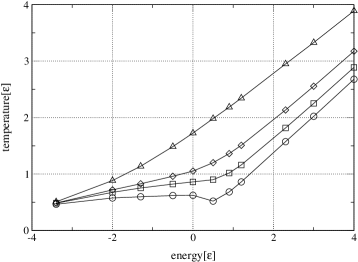
FIG. 1.: In this figure we show the Caloric Curve for 147 Lennard Jones particles for different sizes of the constraining volumes. Circles denote the CC corresponding to a constraining volume of radius $R=15\sigma$ , squares for $R=8\sigma,$ diamonds for $R=6\sigma$ and finally triangles denote the CC for $R=4\sigma$

.

In a recent work we have shown that the effect of confining the excited drop in a given volume, i.e. allowing the system to reach equilibrium, is the appearance of the vapor branch. In this work we will extend those calculations exploring a broader range of densities and incorporing useful dynamical quantities.

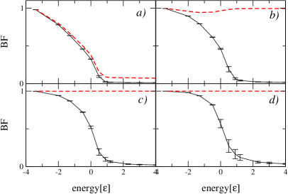
FIG. 2.: In this figure we show the size of the biggest fragment, normalized to the total size of the system, as a function of the energy deposited in the system and for the 4 volumes considered in this work. Panel a) corresponds to a volume of radius $R=15\sigma,$ while b) corresponds to $R=8\sigma,$ c) $R=6\sigma$ and d) $R=4\sigma.$ In each panel two curves are drawn, full lines correspond to fragments recognized by the ECRA formalism, while dotted lines correspond to MST analysis. It can be immediately seen that in the dilute case ($R=15\sigma$) both descriptions give essentially the same result. On the other hand as the system becomes dense the MST comprises most of the mass of the system. This is the reason why as the density is increased the system is not able to separate in different coexisting phases in configurational space. On the other hand, in phase space the system is fragmented irrespective of the value of the density

.

From the analysis of molecular dynamics calculations of constrained systems [8] we have extracted the $CC$s that are displayed in fig.1). It is immediate that a very interesting phenomenon takes place. The same system at the same temperature will change its behavior as a function of the density. In this figure it can be clearly seen that for the less dense case a clear loop in the $CC$ is obtained. But as the density is increased this loop disappears and is replaced by a change in the slope. Moreover at even higher densities the $CC$ looks essentially straight and all signals of a change in behavior are erased.

The origin of the relationship between the $CC$ and the density can be understood quite easily by analyzing the biggest cluster formed in the system. For this purpose we use two algorithms already presented in the literature [13] (see Appendix for details). Very briefly we can say that the, improperly called, Minimum Spanning Tree (MST) algorithm looks for clusters of interacting particles in configuration space, and completely disregards the relative momentum. On the other hand we use the Early Cluster Recognition Algorithm (ECRA) which seeks for the most bound partition in phase space. This algorithm has allowed us to find that the fragmentation in an expanding system takes place very early in the evolution. In fig.2) we show the obtained biggest fragment from the analysis of configurations according to both techniques in constrained systems (see caption for details).

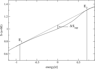
FIG. 3.: In this figure we display the resulting value of the entropy as a function of the energy for a constraining volume of radius $R=15\sigma.$ The curve displays a convex intruder between $E_{1}$ and $E_{2}$ which has been associated with a first order phase transition, $\Delta S$ being the entropy lost in the formation of surfaces. In order to visualize the convex intruder a lineal function $a+b\,E$ has been substracted to the entropy. Here $a=4.3$, $b=1.4$

.

The emerging picture is the following: In the case that the fragment recognition algorithm is the MST, we see that for low densities there is enough room in the constraining volume to allow the formation of drops i.e. At low densities the biggest MST fragment is a decreasing function of the energy. But as we increase the density the biggest MST fragment comprises most of the mass in the system. On the other hand ECRA analysis shows that for all the densities considered the ECRA biggest fragment is a decreasing function of the energy.

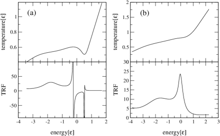
FIG. 4.: Here we show the CC (upper panels) and the associated TRF (lower panels) for two values of the volume. Left hand side correspond to $R=15\sigma$ (dilute case) and right hand side to $R=8\sigma$ (transition to dense state). It can be seen that for the dilute case two poles are present which limit the region of negative TRF. On the other hand at $R=8\sigma$ the TRF is always positive and displays a maximum

.

Once the $CC$ is known it is easy to calculate the Entropy $S$ as a function of the energy and the density.

$$S=\int\frac{dE}{T(E)}$$ (3)

In fig.3) we show $S$ for a dilute system (see caption for details). It is immediate that a convex intruder appears which has been proposed to be a signature of a first order phase transition in non extensive systems. (i.e. the formation of surfaces turns the entropy into a non-extensive function in small systems).

The next step is to calculate the behavior of the Thermal response function of such a system.

$$TRF=\left(\frac{dE}{dT}\right)$$ (4)

In fig.4) the results of such calculation are displayed. We can see that for low densities, as a consequence of the presence of a loop, two poles and negative values are attained by this quantity. This has been signaled as an evidence for a first order phase transition. It is due to the fact that surfaces appear in the system. As the density is increased we reach a threshold above which the $CC$ only displays a change in the slope. Then the two poles merge in a single finite maximum (finite size effect). We can then state that the system goes from a first order like to a second order like behavior as a function of the available space in configuration space.

C Maximum Lyapunov exponent and Asymptotic distance in momentum space

We now proceed with our analysis and focus on the dynamical aspects of the constrained system and its relationship with the above described thermodynamical properties.

One of the main tools to study a chaotic system is the maximum Lyapunov exponent [14], which is a measure of the sensitivity of the system to initial conditions and also gives an idea of the velocity at which the system explores the available phase space. Given two very close initial conditions in phase space, the MLE, ${\hat{\lambda}}$, is given by the following relation :

$$\lambda=\lim_{t\rightarrow\infty}\lim_{d(0)\rightarrow 0}\left[\frac{1}{t}ln\frac{d(t)}{d(0)}\right].$$ (5)

where $d(t)$ is the distance in phase space between two trajectories ($1$ and $2$) which initially differs each other in a very small quantity $d_{0}$.

In order to calculate this quantity we must define a metric:

$$d_{12}(t)=\sqrt{\sum_{i=1,N}\left[a\left(r_{1}\left(t\right)-r_{2}\left(t\right)\right)^{2}+b\left(p_{1}\left(t\right)-p_{2}\left(t\right)\right)^{2}\right]}$$ (6)

In this equation $a$ and $b$ are constants which take care of the units. It has been shown that the $MLE$ are independent of the metric [15]. In our case we have found it useful to take $a=0$ and $b=1/m.$ With m the mass of the particles that according to the units defined in the model gives $b=1.$

If we calculate the distance in momentum space between nearby trajectories we find an exponential growth, followed by a saturation. This saturation is due to the fact that the available phase space is limited (The energy is a constant of motion). In order to handle this we calculate the $MLE$ following a method due to Benettin [16]. In this method, after a time step $\tau<<\tau_{sat}$, the distance $d(\tau)=d_{1}$ is re-scaled to $d_{0}$ in the maximum growing direction and the quantity $ln[d_{1}/d_{0}]$ is saved. Repeating the procedure at every time step $\tau$, the logarithmic increments ${ln[\frac{d_{i}}{d_{i-1}}]}$ are collected. The MLE is defined as:

$$\lambda=\lim_{n\rightarrow\infty}\frac{1}{n\tau}\sum_{i=1}^{n}{ln\left|\frac{d_{i}}{d_{i-1}}\right|}$$ (7)

The ratio $\frac{d_{i}}{d_{i-1}}$ is a measure of the exponential divergence between two initially nearby orbits along the maximum growth direction at time $i\tau$.

Another quantity that has been recently proposed is the $d_{\infty}$ [18, 19]. This is a measure of the maximum distance in momentum space when two initially close trajectories are followed in time. In order to calculate $d_{\infty}$ we use the same metric but no rescaling as in the Benettin method is used. In this case the molecular dynamics evolutions needed to calculate such a quantity are much shorter due to the fact that $d_{\infty}$ reaches a plateau rather fast.

II Results

In what follows we show the results of our calculations.

In first place we show the $MLE$ for constrained systems. In fig.5) we show this quantity for four densities (the same densities at which the $CCs$ are shown in fig.1)). The following features are relevant: For energies below 0, the $MLE$ is an increasing function of the energy, following the behavior of the $CC$. As energy is increased the behavior of the $MLEs$ changes abruptly. In the range $0\lesssim E\lesssim 1$ we find that, for the low density case the $MLE$ displays a very pronounced loop which is in correspondence with the loop displayed by the $CC$. On the other hand for the next two densities a clear loop is present in the $MLE$ while the corresponding $CCs$ only show a change in the slope in this region. Finally for the highest density considered in this work the $CC$ is featureless in this region while the $MLE$ shows a valley.

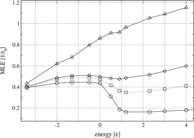
FIG. 5.: In this figure we plot the $MLE$ as a function of the energy deposited in the system for the four values of the constraining volume considered in this work. Symbols have the same meaning as in Fig.1). It can be seen that the $MLE$ clearly signals the transition from a liquid-like regime to a vapor-like regime (according to ECRA analysis)

.

In order to gain insight into the reasons of this behavior we have found it useful to study the following quantities. In first place we look at the mass distributions. When dealing with $MST$ spectra we see that two very different behaviors appear. For $R\lesssim 15\sigma$ fragments (drops) of different sizes appear in the volume as energy is added to the system. The mass spectra goes from extreme U shape in the liquid like region to exponentially decaying in the vapor like region. It is clear that as the density is raised there will be less and less room for the system to form non interacting drops. It is then seen that for $R\gtrsim 8\sigma$ only one $MST$ cluster appears in the system. At this point the $CC$ also shows a change in behavior going from a curve that displays a loop to one that only shows a change in slope. On the other hand when the same configurations are analyzed using the $ECFM$ , via its algorithmic implementation : the $ECRA$ method, a different picture appears: Regardless the size of the constraining walls, the system behaves as undergoing a phase transition, i.e. drops are formed in phase space.

We have also calculated the Normalized Variance of the size of the Maximum fragment ($NVM$). It has been shown [17] that this magnitude will display a maximum for a system whose mass spectra is well described by a scaling law of the type $n_{s}\propto s^{-\tau}f(z)$ at $f(z)=1$. In other words at the point in which the mass distribution is a power law, i.e. a distribution function free of scales. $NVM$ is defined as

$$NVM=\frac{\sigma^{2}\left(BF\right)}{<BF>}$$ (8)

Where $BF$ is the normalized mass of the biggest fragment and the brackets indicate an ensemble averaging. In fig.6) we show the $NVM$ for the four densities considered. It can be readily seen that this quantity displays a maximum in the energy range in which the $MLE$ displays a loop (or a valley for the highest density considered).

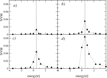
FIG. 6.: Values of the $NVM$ as a function of the energy for the volumes considered in this work. a) corresponds to $R=15\sigma,$ b) to $R=8\sigma,$ c) to $R=6\sigma,$ d) to $R=4\sigma.$ Notice that it displays a clear maximum in all cases which correspond to the region in which an anomaly is detected in the behavior of the $MLE$

.

Now we consider the behavior of the other relevant magnitude presented in this work, i.e. $d_{\infty}.$ In order to explore its scaling properties we define $d_{\infty}^{n}$ which stands for the normalized asymptotic distance

$$d_{\infty}^{n}(t)=\left(\frac{\sum_{i=1}^{N}\left[\left(p_{1}(t)-p_{2}(t)\right)^{2}\right]_{i}}{\frac{1}{2}\sum_{i=1}^{N}\left[p_{1}(t)\right]_{i}^{2}}\right)^{\frac{1}{2}}$$ (9)

In other words

$$d_{\infty}^{n}(t)=\frac{d(t)}{\sqrt{K}}$$ (10)

i.e., the distance in momentum space normalized to the square root of the kinetic energy.

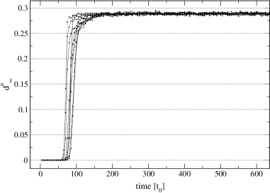
FIG. 7.: $d_{\infty}$ scaled with the square root of the kinetic energy for a volume of radius $R=8\sigma.$ Different curves correspond to different energies in the range $-3.4\leq E\leq 4.0$ Notice that after a short time all the curves collapse into a single one

.

In fig.7) we show the result of such an analysis for $R=8\sigma$ and in fig.8) the same but at $R=15\sigma$ . In both cases it is seen that the asymptotic distance in momentum space scales as the square root of the kinetic energy (and then as the square root of the temperature) of the system as it was conjectured in [18].

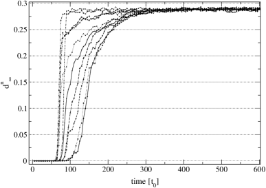
FIG. 8.: Same as Fig 7.) but for a volume of radius $R=15\sigma.$ Notice that, as before, after a still short time, but larger than in the case $R=8\sigma,$ all the curves collapse into a single one

.

Finally in fig.9) we show the $d_{\infty}$ as a function of the energy for two densities. It can be seen that its behavior clearly resembles the corresponding one for the $CC$, thus this quantity could be used instead of T if the latter is not reliably measurable.

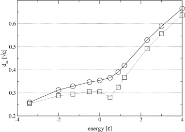
FIG. 9.: In this figure we show $d_{\infty}$ as a function of the energy for volumes corresponding to $R=15\sigma$ (squares) and $R=8\sigma$ (circles). Upon comparison of these curves with the ones corresponding to the CC (fig.1) we can see that both are quite similar

.

III Conclusions

The main results of our calculations can be summarized in the following:

a) The $CC$ is strongly dependent on the density of our system. As the density is increased the behavior of this function goes from displaying a loop (which we refer to as first order like behavior) to one that only presents a change in the slope (in this case we talk about a second order like behavior). In the first case the $TRF$ displays two poles, which converge into a single maximum as the density surpasses a given threshold $(R\sim 8.7\sigma\Rightarrow\rho\sim 0.05\sigma^{-3}).$ Three regions can then be recognized, The liquid like, the transition region and the vapor like region.

b) The $MLE$ is quite sensitive to the transition from liquid like to vapor like states of the finite constrained system. In all cases, even when the $CC$ is almost featureless a signal is detected in the $MLE.$ This signal has been found to be significant by studying other quantities like the $NVM.$

c)The $d_{\infty}$ has been shown to scale like $\sqrt{K}$ and then as the $CC$, giving useful insight into the amount of Phase Space visited by the system.

IV Acknowledgment

This work was partially supported by the University of Buenos Aires (UBA) via grant No tw98, and CONICET via grant No 4436/96.

C.O.Dorso is a member of the carrera del investigador (CONICET), P.Balenzuela is a fellow of the Conicet, M.Ison is a fellow of UBA.

V Appendix

In previous papers the main fragment recognition algorithms currently in use have been fully analyzed [13]. The simplest definition of cluster is basically: a group of particles that are close to each other and far away from the rest. The fragment recognition method known as minimum spanning tree (MST) is based on the last idea (I). In this approach a cluster is defined in the following way: given a set of particles $i,j,k,...$, they belong to a cluster $C$ if :

$$\forall\hskip 5.69046pti\in C\hskip 5.69046pt,\exists\hskip 5.69046ptj\in C\hskip 5.69046pt/\hskip 5.69046pt\left|{\bf r}_{i}-{\bf r}_{j}\right|\leq R_{cl}$$ (11)

where ${\bf r}_{i}$ and ${\bf r}_{j}$ denote the positions of the particles and $R_{cl}$ is a parameter usually referred to as clusterization radius, and is usually related to the range of the interaction potential. In our calculations we took $R_{cl}=3\sigma$.

On the other hand, the early cluster formation model (ECFM) [11], is based on the next definition: clusters are those that define the most bound partition of the system, i.e. the partition (defined by the set of clusters $\{C_{i}\}$) that minimizes the sum of the energies of each fragment according to:

$$E_{\left\{C_{i}\right\}}=\sum_{i}\left[\sum_{j\in C_{i}}K_{j}^{cm}+\sum_{j,k\in C_{i}}V_{j,k}\right]$$ (12)

where the first sum is over the clusters of the partition, and $K_{j}^{cm}$ is the kinetic energy of particle $j$ measured in the center of mass frame of the cluster which contains particle $j$. The algorithm (early cluster recognition algorithm, ECRA) devised to achieve this goal is based on an optimization procedure in the spirit of simulated annealing [11].

REFERENCES

- [1] A.Bonasera, M.Bruno. C.O.Dorso and P.F.Mastinu , Rivista del Nuovo Cimento 23, (2000) 2.
- [2] A.Strachan and C.O.Dorso, Phys. Rev. C 58, (1998) R632.
- [3] F. Gulminelli, Ph. Chomaz, V. Duflot, EuroPhys. Lett. 50, (2000) 434.
- [4] D. H. E. Gross, Microcanonical Thermodynamics, (World Scientific, 2001).
- [5] X. Campi and H.Krivine, arXiv:cond-mat/0005348
- [6] P.Balenzuela, A.Bonasera and C.O.Dorso Phys. Rev.E 62, (1999) 7848.
- [7] A.Strachan and C.O.Dorso, Phys. Rev. C 59, (1999) 285.
- [8] A. Chernomoretz, M.Ison, S.Ortiz and C.O.Dorso, Phys. Rev. C 64, (2001) 024606.
- [9] A.Chernomoretz. C.O.Dorso and J.Lopez, Phys. Rev. C 64, (2001) 044605.
- [10] A.Bonasera, V.Latora and A.Rapisarda, Phys.Rev.Lett. 75, (1995) 3434.
- [11] C.O.Dorso and J. Randrup Phys.Lett.B 301, (1993) 328.
- [12] J.B.Natowitz et al, arXiv:nucl-ex/01060116v2,(2001).
- [13] A.Strachan and C.O.Dorso Phys. Rev. C 56, (1997) 995.
- [14] A.Lichtenberg and M.Lieberman, Regular and Stochastic Motion (Springer-Verlag, 1983).
- [15] V.I.Osedelec, Trans.Moscow.Math.Soc. 19, (1968) 197.
- [16] G.Benettin,L.Galgani and J.M.Strelcyn, Phys.Rev.A 14, (1976) 2338.
- [17] C.O.Dorso, V.Latora and A.Bonasera, Phys.Rev.C 60, (1999) 034606.
- [18] C.O.Dorso and A.Bonasera, Eur.Phys.Jour.A 51 (2001) 421.
- [19] A.Bonasera, V.Latora and M.Ploszajcak, GANIL-preprint(1996)unpublished; V.Baran and A.Bonasera, arXiv:chao-dyn/9804023
- [20] A. Strachan and C. O. Dorso, Phys. Rev. C 55,775 (1997).