Nuclear magnetic dipole properties and the triaxial deformation

Abstract

ABSTRACT: Nuclear magnetic dipole properties of ground bands and $\gamma$-vibrational bands are studied for the first time using the triaxial projected shell model approach. The study is carried out for the Dy and Er isotopic chains, ranging from transitional to well-deformed region. It is found that the g-factor ratio of the $2^{+}$ state in ground bands to that of $\gamma$-bands, $r=g(2^{+},\gamma$-vib)/$g(2^{+},$ ground), varies along an isotopic chain. With the $\gamma$-deformations, which best reproduce the energy levels for both bands, we obtain a qualitative agreement with the experimental data. This result thus suggests that study of the ratio may provide an important information on the triaxial deformation of a nuclear system. The angular-momentum dependence of the ground band g-factor on the triaxial deformation is also investigated.

The importance of triaxial deformation has been a long-standing problem in the studies of atomic nuclei. Although it is known from several model studies that nuclei in the transitional regions acquire a stable triaxial mean-field deformation, consequences of it on the measurable electromagnetic transition probabilities have remained less clear. Nuclear magnetic dipole properties are very sensitive to the single-particle aspects of the nuclear wave-function and hence can provide valuable information on the microscopic structure of a nuclear system. As the single-particle orbits can be strongly modified by triaxiality, the interesting question is whether the triaxial deformation will have observable effects in the magnetic dipole properties.

The study of nuclear magnetic properties has been an active field of research in nuclear structure physics. On the experimental side, considerable progress in the g-factor experiment has recently been made by taking advantages of modern experimental techniques and sensitive detectors, for a recent example, see Ref. [1]. There have been new measurements on the ground band and the $\gamma$-band g-factors for some rare earth nuclei [2, 3]. On the theoretical side, several early calculations were devoted to the study of g-factors. They were based either on the cranking models [4, 5, 6, 7] or on the angular momentum projection method [8, 9, 10]. There have been also calculations using the interacting boson model [11]. However, a microscopic and systematic investigation that treats ground bands and $\gamma$-bands simultaneously, and thus can study their correlations along an isotopic chain, is still missing.

Recently, triaxial projected shell model (TPSM) calculation has become available [12]. The TPSM extends the original projected shell model [13] by removing the restriction of an axially deformed basis assumed in the earlier calculations. In the TPSM approach, one introduces triaxiality in the deformed basis and performs exactly three-dimensional angular momentum projection. In this way, the deformed vacuum state is much enriched by allowing all possible $K$-components. Diagonalization mixes these $K$-states, and various excited levels, specified by $K$, emerge [14]. The first excited TPSM band describes the observed $\gamma$-vibrational band, and the second excited TPSM band reproduces the experimental $\gamma\gamma$-band. This picture is similar to the one shown by Davydov and Filippov [15], but now obtained in terms of a fully microscopic theory. Transition quadrupole moments in $\gamma$-soft nuclei have also been well described by the TPSM [16]. It was shown [16] that the increasing trend in transition quadrupole moment of ground bands has a close relation to the triaxiality of a nucleus.

In the present work, the ground band and the $\gamma$-band g-factors are studied for the first time by using the TPSM. As in the early projected shell model studies [13], to treat these deformed rare earth nuclei, it is appropriate to include three major shells for each type of nucleons ($N=4,5,6$ for neutrons and $N=3,4,5$ for protons). The TPSM wave-function can be written as

$$\Psi^{\sigma I}_{M}=\sum_{K}f^{\sigma I}_{K}\,\hat{P}^{I}_{MK}\,|\,\Phi\!>\,.$$ (1)

In Eq. (1), $\sigma$ specifies the states with the same angular momentum $I$, $\hat{P}^{I}_{MK}$ is the three-dimensional projection operator

$$\hat{P}^{I}_{MK}={2I+1\over 8\pi^{2}}\int d\Omega\,D^{I}_{MK}(\Omega)\,\hat{R}(\Omega),$$ (2)

and $\,|\,\Phi\!>\,$ represents the triaxial qp vacuum state

$$\left\{\hat{P}^{I}_{MK}\,|\,\Phi\!>\,,~{}0\leq K\leq I\right\}.$$ (3)

For studying the low-spin states with $0\leq I\leq 10$ before any quasi-particle (qp) alignment may occur, this is the simplest possible configuration space for an even-even nucleus with the $\gamma$-degree of freedom included.

As in the earlier calculations, we use the pairing plus quadrupole-quadrupole Hamiltonian with inclusion of the quadrupole-pairing term

$$\hat{H}=\hat{H}_{0}-{1\over 2}\chi\sum_{\mu}\hat{Q}^{\dagger}_{\mu}\hat{Q}_{\mu}-G_{M}\hat{P}^{\dagger}\hat{P}-G_{Q}\sum_{\mu}\hat{P}^{\dagger}_{\mu}\hat{P}_{\mu}.$$ (4)

The corresponding triaxial Nilsson Hamiltonian is given by

$$\hat{H}_{N}=\hat{H}_{0}-{2\over 3}\hbar\omega\left\{\epsilon\hat{Q}_{0}+\epsilon^{\prime}{{\hat{Q}_{+2}+\hat{Q}_{-2}}\over\sqrt{2}}\right\}.$$ (5)

In Eq. (4), $\hat{H}_{0}$ is the spherical single-particle Hamiltonian, which contains a proper spin–orbit force [17]. The interaction strengths are taken as follows: The $QQ$-force strength $\chi$ is adjusted such that it has a self-consistent relation with the quadrupole deformation $\epsilon$. The monopole pairing strength $G_{M}$ is of the standard form $G_{M}=\left[21.24\mp 13.86(N-Z)/A\right]/A$, with “$-$” for neutrons and “$+$” for protons, which approximately reproduces the observed odd–even mass differences in this mass region. The quadrupole pairing strength $G_{Q}$ is assumed to be proportional to $G_{M}$, the proportionality constant being fixed as usual to be 0.16. These interaction strengths are consistent with those used previously for the same mass region [12, 13, 14, 16]. $\epsilon^{\prime}$ in Eq. (5) can be adjusted, reflecting how much the system is $\gamma$-deformed. The philosophy of the present approach is that based on the Nilsson potential, one performs explicit angular-momentum projection with a two-body interaction which conforms (through self-consistent conditions) with the mean-field Nilsson potential. The Hamiltonian with separable forces serves only as an effective interaction, the parameters of which have been fitted to the experimental data.

The Hamiltonian in Eq. (4) is diagonalized using the projected basis of Eq. (3). We emphasize that, although only the qp-vacuum state is included in the basis, its triaxial nature generates the $K$-mixing when the diagonalization is carried out. The expansion coefficients $f$, obtained through the diagonalization of the shell-model Hamiltonian, describe the amount of $K$-mixing and specify various physical states (e.g. g-, $\gamma$-, $\gamma\gamma$-bands, $\cdots$) [14].

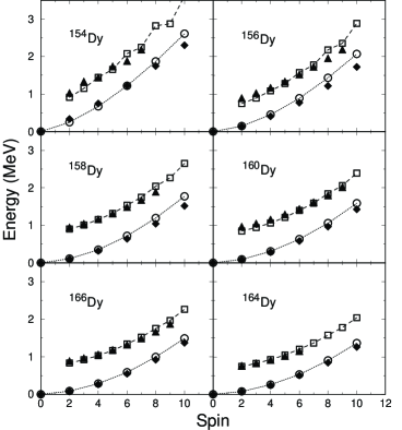
Figure 1: Comparison of calculated energy levels with experimental data for the ground bands and the $\gamma$-band in ^154-164Dy. Filled symbols represent data and open symbols the calculation.

Table 1: Deformation parameters $\epsilon$ and $\epsilon^{\prime}$ used in the TPSM calculations. $\gamma$ are obtained from the relation $\tan\gamma={\epsilon^{\prime}\over\epsilon}$.

Nucleus	$\epsilon$	$\epsilon^{\prime}$	$\gamma$ (degree)
154Dy	0.21	0.120	30
156Dy	0.24	0.130	28
158Dy	0.26	0.120	25
160Dy	0.27	0.125	25
162Dy	0.28	0.130	25
164Dy	0.29	0.140	26

In Fig. 1, we present the calculated energy levels together with experimental data for the ground and the $\gamma$-band in ^154-164Dy. In Table 1, $\epsilon$ and $\epsilon^{\prime}$ used in the TPSM calculations for the Dy isotopes are listed. It can be seen that the TPSM describe the energy levels very well. In particular, the steepness in the increasing curve for the lighter isotopes and the position of the $\gamma$-band head are correctly described in the calculation. In the later discussion for the g-factor calculations, the same deformations $\epsilon$ and $\epsilon^{\prime}$ in Table 1 will be used. We note that changing $\epsilon^{\prime}$ can give different g-factor results, but this will destroy the agreement for the spectrum calculation obtained in Fig. 1.

The wave-functions obtained from the diagonalization are then used to evaluate the electromagnetic transition probabilities. The g-factor $g(\sigma,I)$ is generally defined as

$$g(\sigma,I)=\frac{\mu(\sigma,I)}{\mu_{N}I}=g_{\pi}(\sigma,I)+g_{\nu}(\sigma,I),$$ (6)

with $\mu(\sigma,I)$ being the magnetic moment of a state $(\sigma,I)$. $g_{\tau}(\sigma,I),\tau=\pi$ or $\nu$, is given by

$$g_{\tau}(\sigma,I) = {1\over{\mu_{N}I}}\,<\!\Psi^{\sigma}_{II}|\hat{\mu}^{\tau}_{z}|\Psi^{\sigma}_{II}\!>\,$$

$$= {1\over{\mu_{N}\sqrt{I(I+1)}}}\,<\!\Psi^{\sigma}_{I}||\hat{\mu}^{\tau}||\Psi^{\sigma}_{I}\!>\,$$

$$= \frac{1}{\mu_{N}\sqrt{I(I+1)}}\left(g^{\tau}_{l}\,<\!\Psi^{\sigma}_{I}||\hat{j}^{\tau}||\Psi^{\sigma}_{I}\!>\,+(g^{\tau}_{s}-g^{\tau}_{l})\,<\!\Psi^{\sigma}_{I}||\hat{s}^{\tau}||\Psi^{\sigma}_{I}\!>\,\right).$$

In our calculations, the following standard values for $g_{l}$ and $g_{s}$ [18] have been taken: $g_{l}^{\pi}=1,g_{l}^{\nu}=0,g_{s}^{\pi}=5.586\times 0.75$, and $g_{s}^{\nu}=-3.826\times 0.75$. In the angular-momentum projection theory, the reduced matrix element for $\hat{m}$ (with $\hat{m}$ being either $\hat{j}$ or $\hat{s}$) can be explicitly expressed as

$$\,<\! \Psi^{\sigma}_{I}||\hat{m}^{\tau}||\Psi^{\sigma}_{I}\!>\,$$

$$= \sum_{K_{i},K_{f}}f_{IK_{i}}^{\sigma}f_{IK_{f}}^{\sigma}\sum_{M_{i},M_{f},M}(-)^{I-M_{f}}\left(\begin{array}[]{ccc}I&1&I\\ -M_{f}&M&M_{i}\end{array}\right)\,<\!\Phi|{\hat{P}^{I}}_{K_{f}M_{f}}\hat{m}_{1M}\hat{P}^{I}_{K_{i}M_{i}}|\Phi\!>\,$$

$$= (2I+1)\sum_{K_{i},K_{f}}(-)^{I-K_{f}}f_{IK_{i}}^{\sigma}f_{IK_{f}}^{\sigma}$$

$$\times\sum_{M^{\prime},M^{\prime\prime}}\left(\begin{array}[]{ccc}I&1&I\\ -K_{f}&M^{\prime}&M^{\prime\prime}\end{array}\right)\int d\Omega{\it D}_{M^{\prime\prime}K_{i}}(\Omega)\,<\!\Phi|\hat{m}_{1M^{\prime}}\hat{R}(\Omega)|\Phi\!>\,.$$

We finally have

$$g_{\tau}(\sigma,I) = {1\over{\mu_{N}(I+1)}}\sum_{K_{i},K_{f}}f_{IK_{i}}^{\sigma}f_{IK_{f}}^{\sigma}\sum_{M^{\prime},M^{\prime\prime}}\,<\!IM^{\prime\prime}1M^{\prime}|IK_{f}\!>\,$$

$$\times\int d\Omega{\it D}_{M^{\prime\prime}K_{i}}(\Omega)\,<\!\Phi|\hat{m}_{1M^{\prime}}\hat{R}(\Omega)|\Phi\!>\,.$$

Since wave functions for a ground band and a $\gamma$-band contain different components of the $K$-states, they can have different responses to the triaxiality. As a consequence, one expects different behavior of the g-factors of the states in a ground band and a $\gamma$-band as a function of $\gamma$-deformation. An interesting relation between the ground band and the $\gamma$-band g-factors has been suggested based on experimental information [3], and the departure of the ratio $r=g(2^{+},\gamma$-vib)/$g(2^{+},$ ground) from 1 was interpreted as the $F$-spin admixture within the interacting boson model [19].

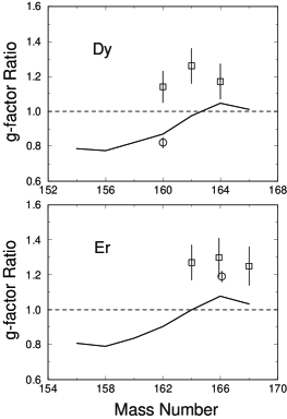
Figure 2: Comparison of calculated g-factor ratio $r=g(2^{+},\gamma$-vib)/$g(2^{+},$ ground) with available data for Dy (top panel) and Er (bottom panel) isotopes. Data are taken from Refs. [2, 3, 20].

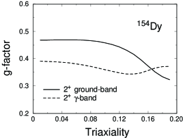
Figure 3: Calculated g-factors of the $2^{+}$ state in the ground band (solid line) and that in the $\gamma$-band (dashed line) for ¹⁵⁴Dy as a function of triaxial deformation $\epsilon^{\prime}$.

In Fig. 2, the calculated g-factor ratios of the $2^{+}$ $\gamma$-state to that of the $2^{+}$ state of ground band are plotted for the Dy and Er isotopic chains. In going from the neutron number $N=88$ to 100, the theoretical curves show the same trend for the two isotopic chains: As the neutron number increases, the ratio $r$ starts from a value around 0.8, goes up and crosses the $r=1$ line, reaches a value close to 1.1, and then turns back. Thus, our theoretical $r$ is clearly smaller than 1 for transitional nuclei, and is close to or larger than 1 for well-deformed nuclei. By collecting available data from the rare earth region, Alfter et al. obtained a similar trend for the experimental $r$ [3]. Unfortunately, there are not sufficient data across the whole isotopic chains for a comprehensive study. In Fig. 2, we plot the available data of the Dy and Er isotopes. For nuclei with the neutron number larger than 96, we have obtained an $r$ value larger than 1, indicating that for these nuclei, the g-factor of the $2^{+}$ $\gamma$-state is larger than that of the $2^{+}$ state of ground band. This is in a qualitative agreement with the existing data. However, the amplitude of the theoretical ratios are smaller than the experimental values. For the nucleus ¹⁶⁰Dy, there have been two independent measurements with rather controversial conclusions [2, 20]. The calculated $r$ value for ¹⁶⁰Dy is close to the one obtained by Alfter et al. in Ref. [20]. The implication of these results is discussed below.

For a better understanding of the above results, let us study the g-factors in terms of the triaxiality in the deformed Nilsson basis and the $K$-mixing among the basis states. In Fig. 3, we plot the g-factors of the $2^{+}$ states in the ground band and the $\gamma$-band for ¹⁵⁴Dy as a function of the triaxial deformation parameter $\epsilon^{\prime}$. It is seen from Fig. 3, that the g-factor of the ground band $2^{+}$ state is significantly larger than that of the $\gamma$-band if the triaxiality $\epsilon^{\prime}$ is small. However, as $\epsilon^{\prime}$ increases, the two g-factors attempt to be close to each other. The two g-factor curves cross eventually at an higher triaxiality around $\epsilon^{\prime}=0.16$. The tendency that the two g-factors get closer for larger $\epsilon^{\prime}$ may be understood as a consequence of the $K$-mixing among the projected $K$-states in Eq. (3). For a small $\epsilon^{\prime}$, the ground band consists of a pure $K=0$ and the $\gamma$-band a pure $K=2$ component. With increasing $\epsilon^{\prime}$, considerable $K=2$ component is mixed into the ground band, and vice versa, $K=0$ component into the $\gamma$-band (see also the discussion in Ref. [14]). For a sufficiently large $\epsilon^{\prime}$, both components can be nearly equally present in the ground band and in the $\gamma$-band. This is the reason to obtain the close values for the two g-factors with large triaxiality.

It becomes clear from Fig. 3 that in our calculation, whether $r$ is larger or smaller than 1, as well as its amplitude, is closely related to the triaxiality $\epsilon^{\prime}$. Changing $\epsilon^{\prime}$ can lead to a different theoretical picture. However, the theoretical $r$ given in Fig. 2 are obtained with the $\epsilon^{\prime}$ that can best reproduce the energy levels in Fig. 1 (for the Er isotopes, in Ref. [14]). $\epsilon^{\prime}$ is related to the conventional triaxial parameter $\gamma$ through the relation $\tan\gamma={\epsilon^{\prime}\over\epsilon}$. The value of $\epsilon$ is held fixed for each nucleus in the calculations, and therefore, $\gamma$ increases linearly with $\epsilon^{\prime}$. We thus suggest that accurate measurement of $r$ can provide useful information for understanding the triaxiality of a nucleus. Experimental study of g-factors is a very challenging task. It is not surprising to see very controversial results from different measurements, such as the example of ¹⁶⁰Dy. We hope that our results will stimulate future g-factor experiments.

Now we turn our discussion to the angular-momentum dependence of the ground band g-factors. Experimental data in Ref. [21] exhibited a significant variation in the g-factors of the low-spin states in some Dy ground bands. The data shows a large drop at $6\hbar$ in ¹⁵⁸Dy and ¹⁶⁰Dy, and a clear jump at $8\hbar$ in ¹⁶²Dy. The early projected shell model calculations [9, 10] with an axially deformed basis did not reproduce the variations. We note that these data are different from those obtained by Brandolini et al. [2, 22] in which these variations were not seen. In the early projected shell model calculations, while the band-crossing with an $i_{13/2}$ neutron pair can be excluded as a cause for these variations [10], there could exist uncertainties due to the restriction of an axially deformed basis. Thus, with the new three-dimensional projection calculation available, the projected shell model results can now be recalculated.

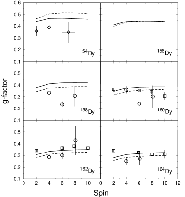
Figure 4: Comparison of available data with calculated g-factors for ^154-164Dy. There are two sets of theoretical curves for calculations with triaxially deformed basis (solid curves) and with axially deformed basis ($\epsilon^{\prime}=0$, dashed curves). The experimental data are taken from Ref. [2] (open squares), Ref. [21] (open circles), and Ref. [23] (open diamonds).

In Fig. 4, results of the TPSM calculations are compared with the experimental data [2, 21, 23] for the isotopes ^154-164Dy. The deformations $\epsilon$ and $\epsilon^{\prime}$ used in the calculations are again those listed in Table 1. It can be seen from Fig. 4 that the theoretical curves appear to be smooth as a function of angular momentum and no variation in the g-factors is obtained. Consequently, the experimental g-factors by Brandolini et al. [2] are nicely reproduced. We can thus conclude that the present calculations, performed with inclusion of $\gamma$-deformed basis and three-dimensional angular momentum projection, can not produce g-factor variations in the low-spin states of ground bands.

In conclusion, the low-spin g-factors of both ground bands and $\gamma$-vibrational bands in the $\gamma$-soft and well-deformed rare earth nuclei have been studied simultaneously using the triaxial projected shell model approach. The diagonalization is carried out in a shell model basis with three-dimensional angular-momentum projection on the triaxially deformed Nilsson-states. It has been shown that the $2^{+}$ state g-factors in ground bands and in $\gamma$-bands behave differently as a function of triaxiality. The g-factor ratio $r$ varies along an isotopic chain, having different characteristic values for transitional and well-deformed nuclei. For a given nucleus, the calculated $r$ can be changed with triaxial deformation. Therefore, we suggest that the ratio of the g-factors, not their dependence on rotation, may be taken as a fingerprint of the nuclear triaxiality. More accurate measurements of the g-factor ratio will be very helpful for a better comparison with the theoretical results presented in this manuscript.

YS thanks the Department of Physics of Tsinghua University for warm hospitality, and for support through the senior visiting scholar program of Tsinghua University. GLL is supported by National Natural Science Foundation of China under Grant No. 10047001, and by China Major State Basic Research Development Program under Contract No. G200077400.

References

- [1] O. Kenn, K.-H. Speidel, R. Ernst, J. Gerber, P. Maier-Komor and F. Nowacki, Phys. Rev. C63 (2001) 064306, and the references cited therein.
- [2] F. Brandolini, M. De Poli, P. Pavan, R.V. Ribas, D. Bazzacco and C.R. Rossi-Alvarez, Eur. Phys. J. A6 (1999) 149.
- [3] I. Alfter, E. Bodenstedt, W. Knichel and J. Schüth, Z. Phys. A355 (1996) 277.
- [4] R. Bengtsson and S. Åberg, Phys. Lett. B172 (1986) 277.
- [5] K. Sugawara-Tanabe and K. Tanabe, Phys. Lett. B207 (1988) 243.
- [6] M.L. Cescato, Y. Sun, and P. Ring, Nucl. Phys. A533 (1991) 455.
- [7] M. Saha and S. Sen, Nucl. Phys. A552 (1993) 37.
- [8] A. Ansari, Phys. Rev. C41 (1990) 782.
- [9] Y. Sun and J.L. Egido, Nucl. Phys. A580 (1994) 1.
- [10] V. Velázquez, J. Hirsch, Y. Sun, and M. Guidry, Nucl. Phys. A653 (1999) 355.
- [11] S. Kuyucak and A.E. Stuchbery, Phys. Lett. B348 (1995) 315.
- [12] J.A. Sheikh and K. Hara, Phys. Rev. Lett. 82 (1999) 3968.
- [13] K. Hara and Y. Sun, Int. J. Mod. Phys. E4 (1995) 637.
- [14] Y. Sun, K. Hara, J.A. Sheikh, J. Hirsch, V. Velázquez, and M. Guidry, Phys. Rev. C61 (2000) 064323.
- [15] A.S. Davydov and F.G. Filippov, Nucl. Phys. 8 (1958) 237.
- [16] J.A. Sheikh, Y. Sun and R. Palit, Phys. Lett. B507 (2001) 115.
- [17] S. G. Nilsson et al., Nucl. Phys. A131 (1969) 1.
- [18] A. Bohr and B.R. Mottelson, Nuclear Structure, Vol. II, Benjamin, New York, 1975.
- [19] J.N. Ginocchio, W. Frank and P. von Brentano, Nucl. Phys. A541 (1992) 211.
- [20] I. Alfter, E. Bodenstedt, W. Knichel and J. Schüth, Z. Phys. A353 (1995) 17.
- [21] I. Alfter, E. Bodenstedt, W. Knichel and J. Schüth, Z. Phys. A357 (1997) 13.
- [22] F. Brandolini, C. Cattaneo, R.V. Ribas, D. Bazzacco, M. De Poli, M. Ionescu-Bujor, P. Pavan and C. Rossi-Alvarez, Nucl. Phys. A600, 272 (1996).
- [23] U. Birkental, A.P. Byrne, S. Heppner, H. Hübel, W. Schmitz, P. Fallon, P.D. Forsyth, J.W. Roberts, H. Kluge, E. Lubkiewicz, and G. Goldring, Nucl. Phys. A555, 643 (1993).