One-body Properties of Nuclear Matter with Off-shell Propagation

Abstract

Symmetric nuclear matter is studied in the self-consistent, in-medium $T$-matrix approach. One-body spectral function, optical potential, and scattering width are calculated. Properties of quasi-particle excitations at the Fermi surface are discussed. Dispersive self-energies are dominated by contributions from the ${}^{1}S_{0}$, $3S_{1}-^{3}D_{1}$, and ${}^{3}P_{1}$ partial waves.

I Introduction

Single-particle properties of nucleons are modified inside the strongly interacting nuclear matterMahaux and Sartor (1991). The optical potential describes the average interaction of a nucleon with the medium. At negative energies, the single-particle potential reflects the modifications of the quasi-particles in the nuclear matter. The spectral function of a nucleon is a measure of the energy distribution of a plane wave state in the system, and can be observed in electron scattering experiments.

Single-particle properties can be calculated from the Brueckner-Hartree-Fock (BHF) theory Köhler (1992); Baldo et al. (1992). Hole-hole diagrams must be added to the lowest order results to obtain a meaningful imaginary part of the self-energy. Because of the violation of the Hugenholz-Van Hove property by the BHF approach, the overall normalization of the single-particle energies is sometimes a problem. BHF calculations use a quasi-particle approximation for the propagators; therefore, a finite order diagram has kinematical limits on the total energy in the scattering. A finite total energy in the interaction could introduce distortions in the far energy tails of the calculated spectral functions.

Recently the in-medium $T$-matrix approximation has been applied to the nuclear matter Vonderfecht et al. (1993); Alm et al. (1996); Dickhoff (1998); Bożek (1999a); Dickhoff et al. (1999); Dewulf et al. (2001); Bozek and Czerski (2001). One obtains nontrivial self-energies by summing a ladder of hole-hole and particle-particle propagators. The self-energies obtained are $\Phi$-derivable Baym (1962); Bozek and Czerski (2001); within this approximation, the single-particle properties are consistent with global thermodynamical properties of the system. A necessary requirement for the in-medium $T$-matrix approach is to use fully self-consistent self-energies and propagators. The propagators are dressed with the imaginary and real parts of the self-energy, and the full spectral function for nucleons must be taken. It requires a serious numerical effort in the calculations, but using a quasi-particle approximation in the $T$-matrix ladder gives too strong pairing Bożek (1999a); Bozek (2000a); Dickhoff et al. (1999), too much scattering Dickhoff et al. (1999); Bożek (1999a), and incorrect single-particle energies Bozek and Czerski (2001).

In the present work we calculate single-particle self-energies and spectral functions using fully self-consistent propagators. We take the complete energy dependence of the self-energies and spectral functions into account in order access reliably the high energy tails of the spectral functions. We present results on the single-particle potential, scattering width and spectral function, obtained with a separable Paris interaction with several partial waves (App. B). In Appendix A we describe in details the numerical methods that allow us to tackle the problem.

We find that normal nuclear density is at the limit of the region of the ${}^{3}S_{1}-^{3}D_{1}$ pairing instability. Owing to the dressing of propagators in the gap equation the superfluid gap is very small, if not vanishing (depending on the details of the interaction in the deuteron channel). We leave the detailed analysis of the pairing in symmetric nuclear matter with realistic interactions to a different work, and study in the following the normal state of nuclear matter.

II In-medium $T$-matrix

In this Section we recall the basic equations of the approach used, more details and discussion can be found in Kadanoff and Baym (1962); Danielewicz (1984); Kraeft et al. (1986); Alm et al. (1996); Vonderfecht et al. (1993); Dickhoff (1998); Bożek (1999a). The $T$-matrix approximation sums ladder diagrams with dressed particle-particle and hole-hole propagators for the in-medium two-particle propagator. The retarded $T$-matrix is

$$\langle{\bf p}|T({\bf P},\Omega)|{\bf p}^{{}^{\prime}}\rangle=V({\bf p},{\bf p}^{{}^{\prime}})$$

$$+\int\frac{d\omega_{1}d\omega_{2}d^{3}q}{32\pi^{5}}V({\bf p},{\bf q})A(p_{1},\omega_{1})A(p_{2},\omega_{2})$$

$$\frac{\big{(}1-f(\omega_{1})-f(\omega_{2})\big{)}}{\Omega-\omega_{1}-\omega_{2}+i\epsilon}\langle{\bf q}|T({\bf P},\Omega)|{\bf p}^{{}^{\prime}}\rangle$$ (1)

where ${\bf p_{1,2}}={\bf P}/2\pm{\bf q}$  and $f(\omega)$ is the Fermi distribution. A partial wave expansion of the in-medium $T$-matrix is performed

$$\langle p|T^{(JST)}_{ll^{{}^{\prime}}}(P,\Omega)|p^{{}^{\prime}}\rangle=V^{(JST)}_{ll^{{}^{\prime}}}({p},{p}^{{}^{\prime}})$$

$$+\sum_{l^{{}^{\prime\prime}}}\int\frac{d\omega_{1}d\omega_{2}q^{2}dq}{8\pi^{4}}V^{(JST)}_{ll^{{}^{\prime\prime}}}({p},{q})$$

$$\langle A(p_{1},\omega_{1})A(p_{2},\omega_{2})\rangle_{P,q}$$

$$\frac{\big{(}1-f(\omega_{1})-f(\omega_{2})\big{)}}{\Omega-\omega_{1}-\omega_{2}+i\epsilon}\langle{q}|T^{(JST)}_{l^{{}^{\prime\prime}}l^{{}^{\prime}}}({P},\Omega)|{p}^{{}^{\prime}}\rangle$$ (2)

after angle averaging the intermediate two-particle propagator ($\langle\dots\rangle=\int\frac{d\Omega}{4\pi}\dots$)

The imaginary part of the retarded self-energy is obtained by closing a pair of external vertices in the $T$-matrix with a fermion propagator

$${\rm Im}\Sigma(p,\omega)=\int\frac{d\omega_{1}d^{3}k}{16\pi^{4}}A(k,\omega_{1})$$

$$\langle({\bf p}-{\bf k})/2|{\rm Im}T({\bf p}+{\bf k},\omega+\omega_{1})|({\bf p}-{\bf k})/2\rangle_{A}$$

$$\Big{(}f(\omega_{1})+b(\omega+\omega_{1})\Big{)}$$ (3)

where

$$A(p,\omega)=~{}~{}~{}~{}~{}~{}~{}~{}~{}~{}~{}~{}~{}~{}~{}~{}~{}~{}~{}~{}~{}~{}~{}~{}~{}$$

$$\frac{-2\mathrm{Im}\Sigma(p,\omega)}{\left(\omega-p^{2}/2m-\mathrm{Re}\Sigma(p,\omega)\right)^{2}+\mathrm{Im}\Sigma(p,\omega)^{2}}$$ (4)

is the self-consistent spectral function of the nucleon and $b(\omega)$ is the Bose distribution. The real part of the self-energy is related to ${\rm Im}\Sigma$ by a dispersion relation

$$\mathrm{Re}\Sigma(p,\omega)=\Sigma_{HF}(p)+{\cal P}\int\frac{d\omega^{{}^{\prime}}}{\pi}\frac{\mathrm{Im}\Sigma(p,\omega^{{}^{\prime}})}{\omega^{{}^{\prime}}-\omega}$$ (5)

with $\Sigma_{HF}(p)$ being the Hartree-Fock self-energy. Eqs. (II), (II), (5) and (II) are to be solved iteratively and at each iteration the chemical potential $\mu$ is adjusted to fulfill the condition on the density

$$\rho=\int\frac{d\omega d^{3}p}{16\pi^{4}}A(p,\omega)f(\omega)=.16\textrm{fm}^{-3}\ .$$ (6)

The $T$-matrix approximation sums ladder diagrams contributing to the ground state energy. In this way it regularizes the short range core in the nucleon interaction similarly as the BHF approach. At the same time, the self-consistent $T$-matrix approximation is $\Phi$-derivable Baym (1962). It was shown for a model interaction that if a fully self-consistent $T$-matrix calculation is performed the thermodynamic consistency relations are fulfilled Bozek and Czerski (2001). In the $T$-matrix approximation a nonzero imaginary self-energy appears and leads to a nontrivial spectral function. It is crucial to keep the full off-shell dependence of the propagators in the calculations. It is possible to treat the resulting energy integrals using numerical methods described in the Appendix A. All the calculations are done using the Fermi energy as the origin of the energy scale. The figures are also plotted using this convention. The calculations are done using a separable parameterization of the Paris potential Haidenbauer and Plessas (1984, 1985). The Fermi energy obtained is $-21.4\textrm{MeV}$ and the binding energy $-15.1\textrm{MeV}$ at normal density. This is not the saturation point for this interaction, but the values quoted above are quite reasonable and give some confidence in the single-particle properties we want to study.

III Optical potential

The real-part of the self-energy defines the single-particle pole in the propagator

$$\omega_{p}=p^{2}/2m+\textrm{Re}\Sigma(p,\omega_{p})\ .$$

The free dispersion relation is modified due to interactions with the medium. The resulting effective potential $\textrm{Re}\Sigma(p,\omega_{p})$ is attractive. It leads in particular to a reduction of the effective mass $m^{\star}=\frac{pdp}{d\omega_{p}}$. We find $m^{\star}\simeq.85m$ at the Fermi momentum, this value depends somewhat on the chosen interaction. The effective mass can be written Mahaux and Sartor (1991) as the product of the $k$-mass $m_{k}/m=\left(1+\frac{m\partial\textrm{Im}\Sigma(k,\omega)}{k\partial k}|_{\omega=\omega_{k}}\right)^{-1}$ and the $\omega$-mass $m_{\omega}/m=\left(1-\frac{\partial\textrm{Im}\Sigma(k,\omega)}{\partial\omega}|_{\omega=\omega_{k}}\right)$. We find $m_{k}/m\simeq.62$ and $m_{\omega}/m\simeq 1.37$ at the Fermi momentum.

The real part of the self-energy is the sum of the Hartree-Fock and the dispersive contribution (5). The real part of the dispersive self-energy is negative around the Fermi energy and around the quasi-particle pole (Fig. 1). The value of the real part of the self-energy on-shell is the effective potential felt by the quasi-particle in the medium. For positive energies of the particle it corresponds to the optical potential.

Figure 1: The real part of the self-energy on-shell (solid line), the Hartree-Fock self-energy (dotted line), and the dispersive part of the self-energy (dashed line).

The depth of the single particle potential is around $-70\textrm{MeV}$ and it is decreasing with momentum. In the range of positive single particle energies ($280\textrm{MeV}<p<500\textrm{MeV}$), the single-particle potential can be fitted with the form Perey and Buck (1962)

$$\textrm{Re}\Sigma(p,\omega_{p})\simeq H_{0}\exp\left(-\beta^{2}k^{2}/4\right)$$

with $H_{0}=-70\textrm{MeV}$ and $\beta=.58\textrm{fm}$ (dashed-dotted line in Fig. 1). The range of nonlocality $\beta$ is small reflecting the fact that the effective mass $m^{\star}$ is not very different from the free one. The depth of the potential for positive energies is consistent with values obtained from phenomenological analyzes of the optical potential Varner et al. (1991). The single particle potential is weakly dependent on the temperature; at $T=4\textrm{MeV}$ $\textrm{Re}\Sigma(p,\omega_{p})$ is shifted up by less than $1\textrm{MeV}$ from its value at zero temperature.

Figure 2: The energy dependence of the single particle potential $\textrm{Re}\Sigma(p,\omega)$ at fixed momentum.

In Fig. 2 is presented the energy dependence of the real part of the self-energy. The energy dependence of the single particle potential is responsible for the time nonlocality of the optical potential. In the whole range of frequencies in Fig. 2 some energy dependence of the potential can be seen. This energy dependence is decreasing with momentum. For energies close to the Fermi energy the energy dependence of the single-particle potential is similar to the one presented in Ref. Baldo et al. (1992). The energy dependence determines the quasi-particle strength

$$Z_{p}=\left(1-\frac{\partial\textrm{Re}\Sigma(p,\omega)}{\partial\omega}|_{\omega=\omega_{p}}\right)\ .$$ (7)

At the Fermi momentum we find $Z_{p_{F}}\simeq.73$. On the other hand, in the range $50\textrm{MeV}<\omega<200\textrm{MeV}$ $\textrm{Re}\Sigma(p,\omega)$ is relatively flat as function of energy.

IV Scattering width

Figure 3: The single particle width $-\textrm{Im}\Sigma(p,\omega)$ as function of energy for $p=0$, $170$, $340$, and $510\textrm{MeV}$; solid, dashed, dotted, and dashed-dotted lines, respectively.

The off-shell scattering width is nonzero on both sides of the Fermi energy but larger at positive energies (Fig. 3). At negative energies the tail of the scattering width extends very far. It is a general feature of self-consistent calculations. Dressed propagators in the $T$-matrix ladder make the imaginary part of the $T$-matrix nonzero even at very negative energies. On the other hand, quasi-particle approximations have a kinematical limit on the lowest energy in the scattering. The scattering width decreases with momentum. It can be understood by the fact that at low momenta the interaction is dominated by the strongest $S$ waves. Other calculations Benhar et al. (1992); Köhler (1992); Baldo et al. (1992); Bozek (2000b); Lehr et al. (2000); Bożek (1999a); Dickhoff et al. (1999); Dewulf et al. (2001) of the variational, BHF, Born, or $T$-matrix type give qualitatively but not quantitatively similar results. The differences are partly due to different short range properties of the interactions used.

Consistently with general features of Fermi liquids at zero temperature, we find that $\textrm{Im}\Sigma(p,\omega=0)=0$ (Fig. 3). The same relation, coming form the restricted phase-space, is fulfilled by other approximations Benhar et al. (1992); Baldo et al. (1992); Lehr et al. (2000). At higher temperatures a nonzero scattering width at the Fermi energy appears.

Figure 4: The temperature dependence of the single particle width $-\textrm{Im}\Sigma(p,\omega=0)$ at the Fermi energy for $p=0$, $170$, $340$, and $510\textrm{MeV}$; solid, dashed, dotted, and dashed-dotted lines, respectively.

As can be seen from Fig. 4 the scattering width at the Fermi energy is increasing as the square of the temperature, as expected from phase space arguments Abrikosov et al. (1963).

The large value of the scattering width above the Fermi energy is due to the short range part of the interaction potential. Splitting the total width into contributions from different partial waves shows that the ${}^{3}S_{1}-^{3}D_{1}$ partial wave is dominant (Fig. 5). For momenta up to twice the Fermi momentum and energies around the Fermi energy, the deuteron partial wave gives by far the most important contribution to the scattering width. It is also in this kinematical region that the overall scattering width is the largest. We have observed a similar large contribution due to this partial wave for the Monagan Mongan (1969) and Yamaguchi Yamaguchi (1954) separable potentials. Consistently, for all these interactions we obtain similar values for $Z_{p_{F}}\simeq.7$. Large values of the scattering width at large energies lead to long tails in the spectral functions.

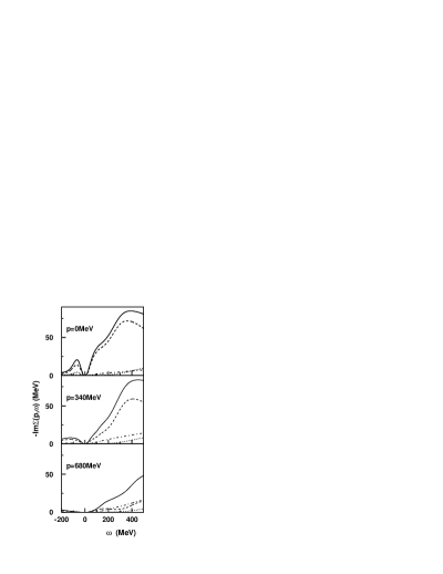
Figure 5: The single particle width $-\textrm{Im}\Sigma(p,\omega)$ as function of energy for $p=0$, $340$, and $680\textrm{MeV}$. The total width is plotted using the solid line. The dashed, dotted, and dashed-dotted lines represent the ${}^{3}S_{1}-^{3}D_{1}$, ${}^{1}S_{0}$, and ${}^{3}P_{1}$ partial waves contributions, respectively.

The imaginary part of the self-energy at the quasi-particle pole is the scattering width of the quasi-particle.

Figure 6: The single particle width $-\textrm{Im}\Sigma(p,\omega)$ at the quasiparticle pole as function of the momentum at $T=0$ (solid line) and $T=4\textrm{MeV}$ (dotted line).

From Fig. 6 we see that around the Fermi momentum, narrow quasi-particle excitation exist. The scattering width behaves as $-\textrm{Im}\Sigma(p,\omega_{p})\propto(p-p_{F})^{2}$, as expected from restricted phase space for scattering Abrikosov et al. (1963). The on-shell scattering width does not reflect the very large values of the off-shell scattering width (Fig. 3). For momenta close to the Fermi surface it is small; and particles with large energies have a scattering probability proportional to the total density and cross section. At finite temperature quasi-particles at the Fermi surface aquire a finite life-time (Fig. 6).

V Spectral function

The role of correlation induced by the medium can be judged by the modifications of the spectral function. Nontrivial, dispersive self-energies lead to broad spectral function with non-Lorentzian shapes and long tails. High energy parts of the spectral functions could be revealed by electron scattering experiments. It is important to calculate the form of the spectral functions including contributions form short range correlations. In Fig. 7 are presented the spectral functions for three representative momenta. For zero momentum the spectral function has a broad peak below and a background part above the Fermi energy. It is the reverse

Figure 7: The spectral function $A(p,\omega)$ as function of energy for $p=0$, $255$, and $350\textrm{MeV}$; solid, dashed, and dotted lines, respectively.

for $p=355\textrm{MeV}$. Following the behavior of the scattering width, the spectral function for any momentum goes to zero at the Fermi energy. For momenta close to the Fermi energy the spectral function has a very sharp peak at the single-particle energy. Its has also a significant background part which cannot be ignored in the sum rules or in the calculation of effective interactions between quasi-particles. Similarly as for the scattering width the self-consistent calculation gives rise to a long tail in the spectral function at negative energies.

The spectral function can be used to obtain the momentum distribution

$$n(p)=\int\frac{d\omega}{2\pi}A(p,\omega)f(\omega)\ .$$ (8)

Short range correlations modifying the spectral function are reflected in the nucleon momentum distribution. The free Fermi distribution is depleted below $p_{F}$ and a high momentum tail in $n(p)$ is formed.

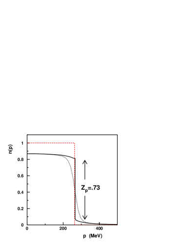
Figure 8: The momentum distribution of nucleons at zero temperature (solid line) and at $T=4\textrm{MeV}$ (dotted line).

At the Fermi momentum the discontinuity in the occupancy is reduced from $1$ to $Z_{p_{F}}$ (7). The Fermi momentum in the interacting system should be the same as in the free one Luttinger (1960); Baym (1962). This relation is approximately fulfilled in the present calculation, but not as well as in our previous work using only $S$ wave interactions Bozek and Czerski (2001). A possible source of the discrepancy could be the use of the partial-wave expansion which spoils the $\Phi$-derivability of the self-energies. At finite temperature the Fermi surface is washed out, but the depletion of the Fermi sea and the high momentum tail are the same. It means that the short range correlations stay essentially the same at $T=4\textrm{MeV}$. The same can also be seen by inspecting the self-energies. At finite temperature the scattering width is increased only in the vicinity of the Fermi energy.

Long tails in the spectral function have implications for saturation properties of nuclear matter. Increased kinetic energy due to the high momentum tail in $n(p)$ is compensated by increased removal energies due to the negative energy tail of the spectral function. A detailed discussion at different densities will be presented elsewhere.

VI Summary

We study the single-particle properties of nucleons in nuclear matter using a conserving, in-medium $T$-matrix approximation. The calculations are done in a self-consistent way with dressed propagators in the ladder diagrams. To our knowledge, it is the first such calculation in the literature using realistic interactions and several partial waves. The full discretization of the spectral function and self-energies allows to discuss the details of their energy dependence. We find that the basic features of a consistent approximation to a Fermi liquid system are fulfilled. The scattering width is zero at the Fermi energy, and the quasi-particles at the Fermi surface have infinite lifetime. The momentum occupancy has a discontinuity of $Z_{p_{F}}$ at the Fermi momentum. The off-shell scattering width is very large at energies $\simeq 300-400\textrm{MeV}$ and momenta below $400\textrm{MeV}$. In this region the main contribution comes from the ${}^{3}S_{1}-^{3}D_{1}$ partial wave. The ${}^{3}P_{1}$ and ${}^{1}S_{0}$ partial waves give also important contributions to the on-shell self-energies. The scattering width on-shell is not very large, maximally $26\textrm{MeV}$. Finite temperature effects are concentrated around the Fermi surface. At finite temperature, the scattering width gets finite around the Fermi energy without modifying the real single-particle potential and the short range correlations. The quasi-particle renormalization factor is $Z_{p_{F}}\simeq.73$ and is largely independent on the interaction used. The effective mass is $m^{\star}\simeq.85m$.

Appendix A Numerical methods

Calculations using self-consistent spectral functions require the evaluation of energy integrals in Eqs. (II) and (II). This is the main numerical difficulty for any self-consistent approximation; only in the last years self-consistent approaches have been applied to the study of high $T_{c}$ superconductors Haussmann (1994); Pedersen et al. (1997); Kyung et al. (1998); Letz and Marsiglio (1999) and nuclear matter Dickhoff (1998); Dickhoff et al. (1999); Bożek (1999a); Bozek and Czerski (2001); Dewulf et al. (2001). Some calculations are performed in the imaginary time formalism Haussmann (1994); Pedersen et al. (1997) which requires a numerical procedure for the analytical continuation to calculate the spectral function. A simpler way is to use the real-time formalism operating with the retarded $T$-matrix, the retarded self-energy, and the spectral function Kyung et al. (1998); Bożek (1999a). The real-time formalism was also used for other calculations of the nuclear matter Dickhoff et al. (1999); Dewulf et al. (2001) performed at zero temperatures. To deal with the off-shell propagation a numerical parameterization of the energy dependence of the spectral function $A(p,\omega)$ by a set of Gaussians has been used Dickhoff (1998); Dickhoff et al. (1999). Alternatively, the spectral function can be represented as a sum of $\delta$ functions Letz and Marsiglio (1999); Dewulf et al. (2001). The above two methods can be easily applied at zero temperature, where a narrow Gausian or one of the $\delta$ functions describes the quasi-particle peak for momenta close to the Fermi surface.

The alternative approach, here employed, uses a direct discretization of the spectral function and self-energies as functions of the energy. If the discretization in $\omega$ is uniform the energy integrals in Eqs. (II) and (II) can be performed efficiently by Fourier transforms. This method can be used directly at finite temperature Bożek (1999a); Kyung et al. (1998), but not for low temperatures where the quasi-particles are very narrow around the Fermi surface (Fig. 6). At zero temperature we have

$$A(p_{F},\omega)=2\pi Z_{p_{F}}\delta(\omega-E_{F})+B(p,\omega)$$ (9)

where the background part $B$ is smooth and can be discretized. Generally, for any momentum close to the Fermi momentum the spectral function is rapidly changing in the vicinity of the quasi-particle peak; therefore, it is has to be split into a quasi-particle peak and a smooth background. The sharp peak is approximated by a $\delta$ function and the smooth part is discretized. We have found numerically that this separation in the spectral function is needed if the width of the quasi-particle peak $-2\textrm{Im}\Sigma(p,\omega_{p})$ is smaller than $\simeq 3$ times the spacing in the energy discretization $\Delta\omega$. We use the following representation of the spectral function

$$A(p,\omega)=2\pi\mathcal{Z}_{p}\delta(\omega-\omega_{p})+B(p,\omega)\ .$$ (10)

The background part is defined as

$$B(p,\omega)=\left\{\begin{array}[]{c}\frac{-2\mathrm{Im}\Sigma(p,\omega)}{(\omega-\omega_{p})^{2}+\mathrm{Im}\Sigma(p,\omega)^{2}}\ ;\\ \text{for}\ (\omega-\omega_{p})^{2}+\mathrm{Im}\Sigma(p,\omega)^{2}>\eta\\ \\ {-2\mathrm{Im}\Sigma(p,\omega)}/{\eta}\ ;\\ \text{for}\ (\omega-\omega_{p})^{2}+\mathrm{Im}\Sigma(p,\omega)^{2}<\eta\end{array}\right.\ .$$ (11)

The parameter $\eta$ is set to cut off the rapidly changing part of the spectral function. We use $\eta\simeq 4\Delta\omega^{2}$. The strength of the quasi-particle component $\mathcal{Z}_{p}$ in Eq. (10) is adjusted to conserve the sum rule $\int\frac{d\omega}{2\pi}A(p,\omega)=1$. The weight of the singular part $\mathcal{Z}_{p}$ is not the same as the renormalization factor $Z_{p}$ (Eq. 7). In Fig. 9 is shown an example of the separation of the background and singular parts of the spectral function $A(p=255\text{MeV},\omega)$.

Figure 9: The spectral function $A(p,\omega)$ as function of the energy (solid line) for $p=240\textrm{MeV}$ and the corresponding smooth background part $B(p,\omega)$ (dashed line). The position of the $\delta$ function representing the quasi-particle peak at $\omega=-7.7\textrm{MeV}$ is indicated by the dotted line.

For a separable interaction $V^{\alpha}(p,p^{{}^{\prime}})=\sum_{i,j}\lambda_{i,j}^{\alpha}g_{i}^{\alpha}(p)g_{j}^{\alpha}(p^{{}^{\prime}})$ the $T^{\alpha}$-matrix for the partial wave $\alpha=(JST)$ is $\langle p|T^{\alpha}(\omega,P)|p^{{}^{\prime}}\rangle=\sum_{i,j}T^{\alpha}_{ij}(\omega,P)g_{i}^{\alpha}(p)g_{j}^{\alpha}(p^{{}^{\prime}})$. Where the matrix $T^{\alpha}_{ij}=(\lambda_{ij}^{\alpha}-J_{ij}^{\alpha})^{-1}$ with the coefficients $J_{ij}^{\alpha}$ given by the integrals

$$J_{ij}^{\alpha}(\Omega,P)=\int\frac{d\omega_{1}d\omega_{2}d^{3}k}{32\pi^{5}}g_{i}^{\alpha}(k)g_{j}^{\alpha}(k)$$

$$\frac{A(p_{1},\omega_{1})A(p_{2},\omega_{2})}{\Omega-\omega_{1}-\omega_{2}+i\epsilon}\left(1-f(\omega_{1})-f(\omega_{2})\right)\ .$$ (12)

Substituting (10) for the spectral functions we have

$${\rm Im}J_{ij}^{\alpha}(\Omega,P)=-\int\frac{d\omega d^{3}k}{32\pi^{4}}g_{i}^{\alpha}(k)g_{j}^{\alpha}(k)B(p_{1},\omega)\left(1-2f(\omega)\right)B(p_{2},\Omega-\omega)$$

$$-\int\frac{d^{3}k}{8\pi^{3}}g_{i}^{\alpha}(k)g_{j}^{\alpha}(k)B(p_{1},\Omega-\omega_{p_{2}}){\cal Z}_{p_{2}}\left(1-f(\Omega-\omega_{p_{2}})-f(\omega_{p_{2}})\right)$$

$$+{\rm Im}\int\frac{d^{3}k}{8\pi^{3}}g_{i}^{\alpha}(k)g_{j}^{\alpha}(k)\frac{{\cal Z}_{p_{1}}{\cal Z}_{p_{2}}\left(1-f(\omega_{p_{1}})-f(\omega_{p_{2}})\right)}{\Omega-\omega_{p_{1}}-\omega_{p_{2}}+i\epsilon}\ .$$ (13)

The energy integral in the first term of Eq. (A) is a convolution of the functions $B(p_{1},\omega)\left(1-2f(\omega)\right)$ and $B(p_{2},\omega)$. It can be evaluated by Fourier transformations using FFT transform algorithms Press et al. (1986). Moreover, the Fourier transform and its inverse can be performed outside of the momentum integral Bożek (1999b). The second term of (A) is a standard two-dimensional integral without singularities. The integral in the last term of (A) is of the type often occurring in quasi-particle calculations, such as the $G$-matrix or the quasi-particle $T$-matrix approximations. Angle averaging separately the numerator and the denominator under the integral we have

$${\rm Im}\int\frac{d^{3}k}{8\pi^{3}}g_{i}^{\alpha}(k)g_{j}^{\alpha}(k)\frac{{\cal Z}_{p_{1}}{\cal Z}_{p_{2}}\left(1-f(\omega_{p_{1}})-f(\omega_{p_{2}})\right)}{\Omega-\omega_{p_{1}}-\omega_{p_{2}}+i\epsilon} \simeq$$

$${\rm Im}\int\frac{k^{2}dk}{2\pi^{2}}g_{i}^{\alpha}(k)g_{j}^{\alpha}(k)\frac{<{\cal Z}_{p_{1}}{\cal Z}_{p_{2}}\left(1-f(\omega_{p_{1}})-f(\omega_{p_{2}})\right)>_{P,k}}{\Omega-<\omega_{p_{1}}+\omega_{p_{2}}>_{P,k}+i\epsilon} =$$

$$-\frac{k_{0}^{2}}{2\pi}\frac{<{\cal Z}_{p_{1}}{\cal Z}_{p_{2}}\left(1-f(\omega_{p_{1}})-f(\omega_{p_{2}})\right)>_{P,k_{0}}}{\partial<\omega_{p_{1}}+\omega_{p_{2}}>_{P,k}/\partial k|_{k=k_{0}}}$$ (14)

where $k_{0}$ is the solution of

$$\Omega=<\omega_{p_{1}}+\omega_{p_{2}}>_{P,k_{0}}\ .$$

The angle average in the denominator $<\omega_{p_{1}}+\omega_{p_{2}}>_{P,k}$ is a function of the total and relative momentum ($P$ and $k$). It can be represented using a one-dimensional function

$$<\omega_{p_{1}}+\omega_{p_{2}}>_{P,k}=\frac{2}{Pk}\left(F(P/2+k)-F(P/2-k)\right)$$ (15)

with

$$F(x)=\int^{{x}}_{0}pdp\omega_{{p}}\ \ .$$

This effectively one-dimensional parameterization allows to perform the integral corresponding to the quasi-particle part of the spectral function very efficiently without using any parabolic approximation for $\omega_{p}$. The same method can also be used in $G$-matrix calculations. The real part of the integrals $J_{ij}^{\alpha}$ is obtained using the dispersion relation

$$\textrm{Re}J_{ij}^{\alpha}(\Omega,P)=\int\frac{\Omega^{{}^{\prime}}}{\pi}\frac{\textrm{Im}J_{ij}^{\alpha}(\Omega^{{}^{\prime}},P)}{\Omega^{{}^{\prime}}-\Omega}\ .$$

The calculation of the energy integral in the equation for the self-energy (II) proceeds very similarly. We have

$${\rm Im}\Sigma(p,\omega)=\int\frac{d\omega_{1}d^{3}k}{16\pi^{4}}B(k,\omega_{1})$$

$$\langle({\bf p}-{\bf k})/2|{\rm Im}T({\bf p}+{\bf k},\omega+\omega_{1})|({\bf p}-{\bf k})/2\rangle_{A}$$

$$\left(f(\omega_{1})+b(\omega+\omega_{1})\right)$$

$$+\int\frac{d^{3}k}{8\pi^{3}}$$

$$\langle({\bf p}-{\bf k})/2|{\rm Im}T({\bf p}+{\bf k},\omega+\omega_{k})|({\bf p}-{\bf k})/2\rangle_{A}$$

$$\left(f(\omega_{k})+b(\omega+\omega_{k})\right)\ .$$ (16)

The energy integral in the first term is again of the form of a convolution and is calculated using Fourier transforms. The integral in the second term is a standard two-dimensional integral. Unlike in the $G$-matrix approximation, the calculation of the self-energy requires the knowledge of the full off-shell $T$-matrix. Restricting oneself to contributions from on-shell $T$-matrix leads to erroneous results Schnell (1996).

In the iteration of the self-consistent set of equations (II, II, II, 5 and 6) it is advantageous to parameterize the energy dependence of the off-shell quantities with respect to the Fermi energy. The iterations are much faster, since a modification of the chemical potential between iterations does not change the most important features of the $\omega$ dependence of $\Sigma(p,\omega)$ and $T(\Omega,P)$, e.g. $\textrm{Im}\Sigma(p,\omega=0)=0$ and the pairing singularity for $T(\Omega=0,P=0)$. The absolute energy scale is recovered only in the calculation of the total density (6) and final observables. This way of proceeding with the iterations can make use of self-energies calculated for other densities or temperatures to start a new iteration.

Appendix B N-N interaction and numerical parameters

We use a separable parameterization of the Paris potential Haidenbauer and Plessas (1984, 1985). It contains all the $J=0$, $J=1$, $J=2$, and the ${}^{3}D_{3}-^{3}G_{3}$ partial waves. For the most important ${}^{1}S_{0}$ and ${}^{3}S_{1}-^{3}D_{1}$ partial waves we choose the rank $3$ and $4$ respectively. We have observed that the use of the separable parameterization of the Paris potential for the ${}^{3}P_{1}$ partial wave leads to very high values of the effective mass $m^{\star}\simeq.95m$. Since the ${}^{3}P_{1}$ phase shifts are not well reproduced by the parameterization of Ref. Haidenbauer and Plessas (1984), we choose the Mongan $I$ parameterization Mongan (1969) for this partial wave. It is important to check that no unphysical bound states occur in the off-shell $T$-matrix for the given choice of $N-N$ potentials. The contribution from such unphysical bound states, even far from the considered on-shell energies, would spoil the calculated self-energies.

The use of the Fourier transform algorithm for the calculation of energy integrals requires a fixed spacing in the energy grid. It means that we have to set finite ranges for the kinematical variables in the model. The single particle momenta are in the range $p<1700\textrm{MeV}$. The total momentum of a nucleon pair is limited by $3400\textrm{MeV}$. The energy dependence of the $T$-matrix $T(\Omega,P)$ is calculated for $-2500\textrm{MeV}+P^{2}/4m<\Omega<3500\textrm{MeV}$. The energy range for the single particle self-energy is taken from $-1700\textrm{MeV}$ to $3500\textrm{MeV}$. The energy dependent functions are discretized with a grid spacing of $1.28\textrm{MeV}$.

To obtain results with stability between iterations better than $1\%$ we need typically 7 iterations at zero temperature. The convergence of the iterations is faster and more stable at finite temperature.

References

- Mahaux and Sartor (1991) C. Mahaux and R. Sartor, in Advances in Nuclear Physics, edited by J. W. Negele and E. Vogt (Plenum Press, New York, 1991), vol. 20, pp. 1–223.
- Baldo et al. (1992) M. Baldo, I. Bombaci, G. Giansiracusa, U. Lomabrdo, C. Mahaux, and R. Sartor, Nucl. Phys. A545, 741 (1992).
- Köhler (1992) H. S. Köhler, Phys. Rev. C46, 1687 (1992).
- Dickhoff (1998) W. H. Dickhoff, Phys. Rev. C58, 2807 (1998).
- Bożek (1999a) P. Bożek, Phys. Rev. C59, 2619 (1999a), eprint [http://arXiv.org/abs]nucl-th/9811073.
- Vonderfecht et al. (1993) B. Vonderfecht, W. Dickhoff, A. Polls, and A. Ramos, Nucl. Phys. A555, 1 (1993).
- Bozek and Czerski (2001) P. Bozek and P. Czerski, Eur. Phys. J. A11, 271 (2001), eprint [http://arXiv.org/abs]nucl-th/0102020.
- Dickhoff et al. (1999) W. H. Dickhoff, C. C. Gearhart, E. P. Roth, A. Polls, and A. Ramos, Phys. Rev. C60, 064319 (1999).
- Dewulf et al. (2001) Y. Dewulf, D. Van Neck, and M. Waroquier, Phys. Lett. B510, 89 (2001), eprint [http://arXiv.org/abs]nucl-th/0012022.
- Alm et al. (1996) T. Alm, G. Röpke, A. Schnell, N. H. Kwong, and H. S. Kohler, Phys. Rev. C53, 2181 (1996), eprint [http://arXiv.org/abs]nucl-th/9511039.
- Baym (1962) G. Baym, Phys. Rev. 127, 1392 (1962).
- Bozek (2000a) P. Bozek, Phys. Rev. C62, 054316 (2000a), eprint [http://arXiv.org/abs]nucl-th/0003048.
- Kadanoff and Baym (1962) L. Kadanoff and G. Baym, Quantum Statistical Mechanics (Bejamin, New York, 1962).
- Kraeft et al. (1986) W. D. Kraeft, D. Kremp, W. Ebeling, and G. Röpke, Quantum Statistics of Charged Particle Systems (Plenum Press, New York, 1986).
- Danielewicz (1984) P. Danielewicz, Annals Phys. 152, 305 (1984).
- Haidenbauer and Plessas (1984) J. Haidenbauer and W. Plessas, Phys. Rev. C30, 1822 (1984).
- Haidenbauer and Plessas (1985) J. Haidenbauer and W. Plessas, Phys. Rev. C32, 1424 (1985).
- Perey and Buck (1962) F. Perey and B. Buck, Nucl. Phys. 32, 353 (1962).
- Varner et al. (1991) R. L. Varner, W. J. Thomson, T. L. McAbee, E. J. Ludwig, and T. B. Clegg, Phys. Rep. 201, 57 (1991).
- Benhar et al. (1992) O. Benhar, A. Fabrocini, and S. Fantoni, Nucl. Phys. A550, 201 (1992).
- Bozek (2000b) P. Bozek, in International Workshop On Kadanoff-Baym Equations: Progress And Perspectives For Many-Body Physics, edited by M. Bonitz (World Scientific, Singapore, 2000b), eprint [http://arXiv.org/abs]nucl-th/9910022.
- Lehr et al. (2000) J. Lehr, M. Effenberger, H. Lenske, S. Leupold, and U. Mosel, Phys. Lett. B483, 324 (2000).
- Abrikosov et al. (1963) A. A. Abrikosov, L. P. Gorkov, and I. E. Dzyaloshinski, Methods of Quantum Field Theory in Statistical Physics (Prentice-Hall Inc., New Jersey, 1963).
- Mongan (1969) T. R. Mongan, Phys. Rev. 178, 1597 (1969).
- Yamaguchi (1954) Y. Yamaguchi, Phys. Rev. 95, 1628 (1954).
- Luttinger (1960) J. M. Luttinger, Phys. Rev. 119, 1151 (1960).
- Haussmann (1994) R. Haussmann, Phys. Rev. B49, 12975 (1994).
- Pedersen et al. (1997) M. H. Pedersen, J. J. Rodríguez-Núñez, H. Beck, T. Schneider, and S. Schafoth, Z. Phys. B103, 21 (1997).
- Kyung et al. (1998) B. Kyung, E. G. Klepfish, and P. E. Kornilovitch, Phys. Rev. Lett. 80, 3109 (1998).
- Letz and Marsiglio (1999) M. Letz and F. Marsiglio, J. Low. Temp. Phys. 117, 149 (1999).
- Press et al. (1986) W. Press, S. A. Teukolsky, W. T. Vetterling, and B. P. Flannery, Numerical Recipes in Fortran 77 (Cambridge University Press, Cambridge, 1986).
- Bożek (1999b) P. Bożek, Nucl. Phys. A657, 187 (1999b), eprint [http://arXiv.org/abs]nucl-th/9902019.
- Schnell (1996) A. Schnell, Ph.D. thesis, Rostock University (1996).