THERMAL DESCRIPTION OF PARTICLE PRODUCTION IN ULTRA-RELATIVISTIC HEAVY-ION COLLISIONS

ABSTRACT

The grand-canonical version of the thermal model is used to analyze the ratios of particle abundances measured in ultra-relativistic heavy-ion collisions. Exactly the same model is applied to study the heavy-ion reactions at BNL AGS, CERN SPS, and BNL RHIC. A very good description is achieved for Pb + Pb collisions at CERN SPS and for Au + Au collisions at BNL RHIC. In these two cases the value of the temperature characterizing the chemical freeze-out is practically the same: we find $T_{chem}=168\pm 3$ MeV at SPS, and $T_{chem}=165\pm 7$ MeV at RHIC. On the other hand, the particle ratios measured in the collisions of lighter nuclei are described only in the qualitative way. We discuss also the effect of the possible in-medium modifications of hadron masses and widths on the thermal fits. For Pb + Pb collisions at CERN SPS and Au + Au collisions at BNL RHIC, we find that the $\chi^{2}$ fits favor slightly a moderate, $\sim$ 20%, decrease of the masses. In this case, the fits with the modified masses yield modified values of the optimal temperature and the baryon chemical potential. In-medium modifications of the widths have little effect on the fits, unless they are increased by a factor larger than 2. We study in detail the thermodynamic conditions characterizing the chemical freeze-out. In particular we find that the average baryon energy at freeze-out is 1.6 GeV, and the average meson energy is 0.9 GeV. This difference reflects a different behavior of the mass spectra of baryons and mesons. Similarities and differences between our calculations and other studies are thoroughly discussed.

Chapter 1 Introduction

1.1 Ultra-Relativistic Heavy-Ion Collisions

The field of the ultra-relativistic heavy-ion collisions connects the nuclear physics with the elementary particle physics. In the high-energy particle physics the interactions are derived from first principles (local gauge theories) and one deals with single particles (leptons, hadrons, or quarks and gluons). On the other hand, in the traditional nuclear physics the strong interaction is described by effective models, and the matter consists of extended complicated systems (nuclei). A unifying aspect of the high-energy nuclear collisions is an attempt to analyze the properties of dense hadronic matter in terms of elementary interactions. The fundamental theory of strong interactions, Quantum Chromodynamics (QCD), predicts that at high energy density, hadronic matter will turn into a plasma of deconfined quarks and gluons (QGP). The search for such a phase transition is the main motivation for the continuous experimental and theoretical efforts in the field [1-8]. One of the goals of the experimental program is to recreate (on a microscopic scale) the physical conditions that are thought to have existed in the early universe. Such astrophysical aspect of the ultra-relativistic heavy-ion collisions indicates once again on the interdisciplinary character of this new branch of physics.

The experimental studies of the high-energy nuclear collisions started in 1986 at the Brookhaven National Laboratory (BNL) and at the European Organization for Nuclear Research (CERN). The Alternating Gradient Synchrotron (AGS) at BNL accelerated ²⁸Si beams (at 15 GeV per nucleon) and later ¹⁹⁷Au beams (at 11 GeV per nucleon). At CERN the Super Proton Synchrotron (SPS) delivered ¹⁶O and ³²S beams (at 60 and later at 200 GeV per nucleon), which were followed in 1995 by ²⁰⁸Pb beams (at 158 GeV per nucleon). The new era in the field started in 2000, when the Relativistic Heavy Ion Collider (RHIC) started operation at BNL. In the first run of RHIC, Au on Au reactions were studied at the center-of-mass energy $\sqrt{s}=$ 56 A GeV and $\sqrt{s}=$ 130 A GeV. In 2001, during the second run the full collision energy, $\sqrt{s}=$ 200 A GeV, and the full luminosity were achieved.

Over the last 15 years, the large amount of data has been accumulated. In particular, the data indicate that the hadronic matter at freeze-out (i.e., at the moment when the hadron interactions cease and the particles freely stream from the collision point to the detectors) is well described by the equilibrium distributions [9-23]. In addition, as one moves up from SPS to RHIC energy, approximately the same temperature and a significantly smaller baryonic chemical potential is observed in the central rapidity region. This fact constrains different possible models of the particle production. Actually, there is no single space-time model describing the whole collision process, since different degrees of freedom are important at different stages of a collision. As a consequence, each stage requires a different treatment: The initial moments are described with the help of partonic degrees of freedom (quarks and gluons). The intermediate stage is described typically in the framework of the relativistic hydrodynamics (in this case the degrees of freedom are collectively included in the equation of state). Finally, the last stage is described in purely hadronic models.

place	projectile	target(s)	$E_{lab}/A\,\,$[GeV]	$y_{lab}$	$\sqrt{s}/A$  [GeV]
BNL  AGS	Si	Au, Pb	14.6	3.4	5.4
CERN  SPS	S	Au, W, Pb	200	6.1	19.4
CERN  SPS	Pb	Pb	158	5.8	17.3
BNL  RHIC	Au	Au	$\left(\begin{tabular}[]{c}9000\\ 21300\end{tabular}\right)$	$\left(\begin{tabular}[]{c}9.9\\ 10.7\end{tabular}\right)$	130 200

Table 1.1: Heavy-ion reactions studied in this paper.

1.2 Aim of this Work

In this work we discuss the properties of matter at freeze-out, thus we are not interested in the microscopic mechanism of particle production, such as decaying color strings [24] or a parton cascade [25]. We assume, however, that the real microscopic mechanism leads finally to creation of a locally equilibrated hadron gas. We note that in our approach one cannot draw any direct conclusions concerning formation of the quark-gluon plasma at the earlier stages of a collision. Such information is lost in the thermal equilibrium, which has no memory about earlier times.

Our main purpose is to perform a thermal analysis of the particle yields. We are going to check whether the measured particle yields may be explained in a model which assumes full thermal and chemical equilibrium of the hadronic matter at freeze-out. In the last years such thermal approach has been used by several groups to study different types of reactions. The results of such investigations show that the thermal description of the particle production is quite successful. We have to have in mind, however, that different groups use different implementations of the model, and these implementations vary for each particular reaction. In this situation, the conclusions drawn from the vast applications of the thermal models may be not completely consistent. In this paper, to minimize such effects, one formulation of the model is used to describe most of the available data. In this way, exactly the same thermodynamic features of the particle production are used to characterize different collisions. This allows us to observe similarities and differences in the thermodynamic behavior of various colliding systems.

The second and independent aim of this work is to include the possible in-medium modifications of hadron properties into the thermal approach. In the scenario with the two different freeze-outs, i.e., with the chemical freeze-out preceding the thermal freeze-out, the study of the particle ratios reveals the information about the chemical freeze-out: the concept of the chemical freeze-out refers to the point at which inelastic collisions cease and all particle ratios are frozen, whereas the concept of the thermal freeze-out refers to the stage when all elastic collisions cease. If the hadronic matter at the chemical freeze-out is very hot and dense, we may take into account the mass and width modifications of hadrons. Such modifications are predicted by the effective theories of QCD [26-29], and also by the QCD sum rules in medium [30]. For instance, according to Brown and Rho [31], the masses of hadrons decrease at higher densities. The change of the mass leads to a change of the hadron densities, which should be reflected in the measured relative particle yields. The study of such effects is the second important issue discussed in the present paper.

In our study of the particle multiplicities we use our own implementation of the thermal model, which has been constructed as a code in the MATHEMATICA language. The use of the symbolic manipulations allowed by the MATHEMATICA turned out to be very convenient in the treatment of the hadronic decays. Creation of this code was the main technical task connected with the present investigations. A part of the original results discussed in this paper has been published before in the two articles:

• M. Michalec, W. Florkowski, and W. Broniowski: Scaling of hadron masses and widths in thermal models for ultra-relativistic heavy-ion collisions, Phys. Lett. B520 (2001) 213; nucl-th/0103029.

• W. Florkowski, W. Broniowski, and M. Michalec: Thermal analysis of particle ratios and $p_{\perp}$ spectra at RHIC, nucl-th/0106009.

Chapter 2 Thermal Model of Particle Production

2.1 Historical Perspective

The use of statistical concepts to describe particle production in hadronic collisions has a long history. In the early fifties Fermi [32] assumed that when two relativistic nucleons collide, the energy available in their center-of-mass system is released in a very small volume (due to the Lorentz contraction). Subsequently, such a dense system decays into one of many accessible multiparticle states. The decay probabilities were calculated by Fermi according to the standard rules of statistical mechanics. In the Landau’s hydrodynamic model the picture of the instantaneous break-up was modified by the inclusion of the expansion stage. The volume expansion leads to cooling and lowering of the freeze-out temperature, and causes that most final hadrons are the light ones.

In the Landau hydrodynamic model [33] the initial conditions are specified at a given time, when the matter is highly compressed and at rest. This description does not include one aspect of the particle production at high energies, namely, the fact that fast particles are produced later and farther away from the collision center than slow particles. This feature of particle production has been included in the Bjorken [34, 35] hydrodynamic model which imposes boost-invariant initial conditions.

Thermal and/or statistical interpretation of the particle production became a common approach for the ultra-relativistic heavy-ion collisions [9-23]. In this case large numbers (multiplicities) of hadrons are created, and the statistical methods seem to be appropriate. Of course, the produced matter may be formed in a state which is far away from the local equilibrium, so the use of the simple equilibrium concepts must be grounded in more involved studies using, e.g., the kinetic theory of hadronic matter.

2.2 Thermal and Chemical Freeze-Out

In the simplest version of the thermal model one assumes that the hadronic matter created in nuclear collisions forms an ideal gas. A volume expansion of the gas, caused by high internal pressure, leads to decoupling or freeze-out of the hadrons. This process takes place when the mean free path of hadrons becomes compatible with the macroscopic size of the whole hadronic system. After the freeze-out, the particles move freely and their properties may be measured in the detectors. If the freeze-out process is fast, the momentum distributions of the particles do not change substantially, and the measured spectra have thermal shapes. Thus, by studying the hadron momentum distributions we may check the validity of the concept of thermalization. Moreover, in the thermal model the abundances of different hadron species are fixed by the values of a few thermodynamic parameters. Consequences of this fact can be verified by the measurements of the relative particle yields.

More realistically, the hadronic system at the freeze-out can be viewed as a collection of subsystems. Each of such subsystems can be characterized by the individual (or local) values of the thermodynamic parameters, and by the individual value of the collective velocity. The case described above corresponds to the situation when all local thermodynamic parameters are the same, and the collective velocities are small. In this approximation the measurements of the momentum distributions and of the relative yields should reveal the same value of the temperature and the same values of the chemical potentials. On the other hand, if the collective velocities are not negligible, the momentum spectra of hadrons are modified by a superposition of ”redshift” and ”blueshift” effects. The spectra do not reveal the true local freeze-out conditions anymore. It can been shown, however, that the measurement of the relative particle yields is not affected by the collective velocities, provided the local thermodynamic parameters are the same [36, 37]. This crucial observation makes grounds for a large interest in the studies of the particle ratios. In this paper we follow this trend and perform thermal analysis of the particle ratios measured at BNL AGS, CERN SPS, and BNL RHIC.

Since the thermal fits to the particle ratios give quite large values of the optimal temperature, one finds typically $T\sim$ 170 MeV, a concept of the two different freeze-outs has been introduced: at first the chemical freeze-out takes place, and only later the thermal (or kinetic) freeze-out happens. At the chemical freeze-out the chemical contents of the hadronic system is established. Later, only elastic processes are possible (dominate), leading to further expansion of the system and cooling. Finally, when the system becomes sufficiently diluted, the true thermal freeze-out takes place (as described above). The concept of the two freeze-outs helps to understand the large difference between the temperature inferred from the investigation of the particle ratios, and the temperature inferred from the study of the momentum distributions. At SPS energies, the temperature of the thermal freeze-out  is around $T\sim$130 MeV. A detailed study of the freeze-out mechanism can be performed only in the microscopic framework, such as the relativistic kinetic theory. In our approach, we simply adopt the definition of the chemical freeze-out and check if the particle multiplicities measured in the ultra-relativistic heavy-ion collisions are consistent with this idea.

It should be noticed, however, that there exist models of hadron production in ultra-relativistic heavy-ion collisions, which assume that the chemical freeze-out coincides with the thermal freeze-out. An example of such a model is the sudden hadronization scenario of Ref. [22]. Another model with a single freeze-out is defined in Ref. [23]. We want to emphasize that in this case (i.e., in the situations when a single freeze-out is considered) our calculations are also useful for the determination of the thermodynamic properties of hadronic matter. For example, the results of our analysis of the particle ratios at RHIC [21] were combined with the hydrodynamic expansion in order to calculate the transverse-momentum spectra of hadrons [23]. This approach yields very successful fits and shows that the thermal analysis of the ratios may be the first step in more complex investigations of other observables such as elliptic flow or HBT radii.

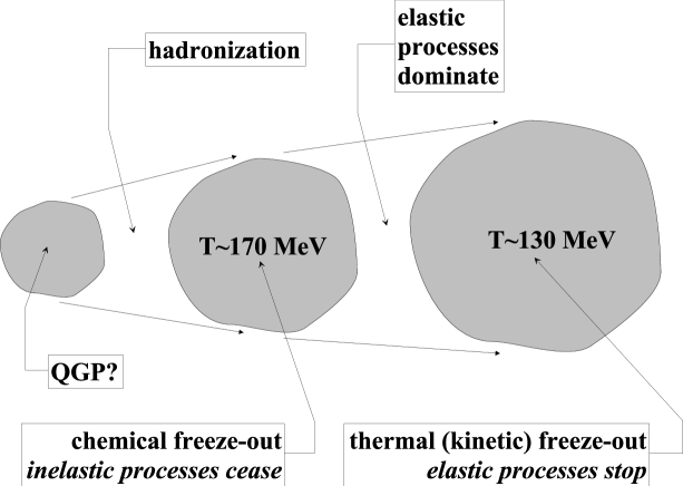
Figure 2.1: In many scenarios of the evolution of the hadronic matter in ultra-relativistic heavy-ion collisions, the chemical freeze-out precedes the thermal (kinetic) freeze-out. At the chemical freeze-out the inelastic processes stop and the chemical content of the fireball is established. Later on, only elastic processes are present. They lead to further expansion and cooling of the system. At the thermal freeze-out the elastic interactions cease, and the particles stream freely to detectors. A high temperature of the chemical freeze-out suggests that it happens just after hadronization of the quark-gluon plasma possibly created in the collisions.

2.3 Basics of Thermal Analysis

2.3.1 Static Fireball

In this Section we give the basic formulas used in the thermal analysis of the particle ratios. We start with the presentation of the simplest approach and assume that the (chemical) freeze-out takes place in a static volume. In this case the multiplicities of hadrons of species $i$ are obtained from the ideal-gas expression

$$N_{i}=Vn_{i}=Vg_{i}\int d^{3}p\ f_{i}\left(p\right).$$ (2.1)

Here $V$ is the volume of the hadronic system at the freeze-out, $g_{i}=2J_{i}+1$ is the spin degeneracy factor of the $i$th hadron, and $f_{i}(p)$ is the momentum distribution function. In the thermodynamic equilibrium the distribution functions $f_{i}(p)$ have a form ($\hbar=1$)

$$f_{i}\left(p\right)=\frac{1}{\left(2\pi\right)^{3}}\left[\exp\left(\frac{E_{i}(p)-\mu_{i}}{T}\right)+\epsilon\right]^{-1},$$ (2.2)

where

$$E_{i}(p)=\sqrt{p^{2}+m_{i}^{2}}$$ (2.3)

is the energy, $T$ is the temperature, and $\mu_{i}$ is the chemical potential. The quantity $\epsilon$ equals +1 for fermions (in this case (2.2) becomes the Fermi-Dirac distribution) and -1 for bosons (in this case (2.2) becomes the Bose-Einstein distribution). The limit $\epsilon\longrightarrow 0$ corresponds to the classical (Boltzmann) statistics. The chemical potential $\mu_{i}$ in Eq. (2.2) is a linear combination of the baryon, strange and isospin chemical potential

$$\mu_{i}=\mu^{B}B_{i}+\mu^{S}S_{i}+\mu^{I}I_{i}.$$ (2.4)

Here $B_{i},S_{i},$ and $I_{i}$ are the baryon number, strangeness, and the third component of isospin of the $i$th hadron, respectively.

Introduction of the chemical potentials $\mu^{B},\mu^{S}$ and $\mu^{I}$, allows us to fulfill the appropriate conservation laws. We assume that the strangeness of the system is zero

$$\sum_{i}S_{i}N_{i}=0,$$ (2.5)

and the ratio of the electric charge to the baryon number in the hadronic fireball is the same as in the colliding nuclei

$$\frac{\sum_{i}Q_{i}N_{i}}{\sum_{i}B_{i}N_{i}}=\frac{Z}{A}.$$ (2.6)

Here $Q_{i}$ is the electric charge of the $i$th hadron. According to the Gell-Mann – Nishijima formula we have

$$Q_{i}=I_{i}+\frac{\left(B_{i}+S_{i}\right)}{2}.$$ (2.7)

In the practical calculations, Eqs. (2.5) and (2.6) are used to fix the values of the chemical potentials $\mu^{S}$ and $\mu^{I}$. Thus, we are left with only two independent parameters: the temperature and the baryon chemical potential. We note that the volume cancels in the conditions (2.5) and (2.6), and also in the particle ratios introduced below. The values of $Z$ and $A$ (for the nuclei discussed in our paper) are given in the Table 2.1.

	Si	S	W	Au	Pb
$Z$	14	16	74	79	82
$A$	29	32	184	197	207
$Z/A$	0.48	0.50	0.40	0.40	0.40

Table 2.1: The values of the atomic numbers, $Z$, and the mass numbers, $A$, for the nuclei discussed in the present paper.

2.3.2 Expanding Fireball

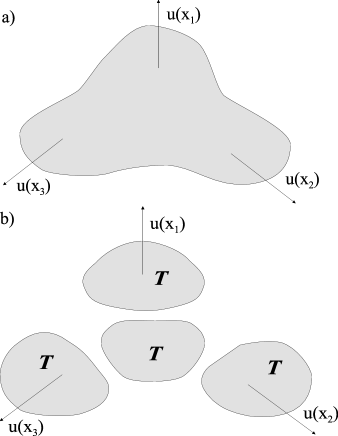
Figure 2.2: Illustration of the insensitivity of the particle ratios to hydrodynamic flow. An expanding system (a) can be viewed as a collection of subsystems (b) which move with collective velocities $u(x)$. If the thermodynamic potentials are the same in each subsystem, the particles are emitted in identical proportions. In this case the measurement of the yields in the full phase-space reveals the local thermodynamic conditions.

In a more general case, when the expansion of the system at freeze-out cannot be neglected, one may use the Cooper-Frye formula [38, 39] to calculate the total yield of particles of species $i$, namely

$$N_{i}=\int\frac{d^{3}p}{E_{i}(p)}\int d\Sigma_{\mu}\,\,p^{\mu}\,\,g_{i}\ f_{i}\left(\sqrt{\left(p\cdot u\right)^{2}-m_{i}^{2}}\right).$$ (2.8)

Here $\Sigma_{\mu}$ describes the element of the freeze-out hyper-surface, and $u^{\mu}$ is the local hydrodynamic four-velocity. In the local rest frame: $u^{\mu}=(1,0,0,0)$ and $\sqrt{\left(p\cdot u\right)^{2}-m_{i}^{2}}=p$. Both $\Sigma_{\mu}$ and $u^{\mu}$ depend on the space-time position $x$. In general, also $T$ and $\mu_{i}$ may be defined locally.

Eq. (2.8) can be rewritten in terms of the number current [36]

$$N_{i}=\int d\Sigma_{\mu}(x)\,j_{i}^{\mu}(x),$$ (2.9)

where

$$j_{i}^{\mu}\left(x\right) = 2\int d^{4}p\,\theta\left(p^{0}\right)\delta\left(p^{2}-m_{i}^{2}\right)p^{\mu}\,\,g_{i}\ \,f_{i}\left(\sqrt{\left(p\cdot u\right)^{2}-m_{i}^{2}}\right)$$ (2.10)

$$= 2\int d^{4}p\,\theta\left(p^{0}\right)\delta\left(p^{2}-m_{i}^{2}\right)p^{\mu}\,\,g_{i}\left[\exp\left({p\cdot u-\mu_{i}\over T}\right)+\epsilon\right]^{-1}.$$

Eq. (2.10) is written in a manifestly Lorentz-covariant way. The step function $\theta(x)$ is defined by the conditions

$$\theta(x)=1\,\,\,\hbox{for}\,\,\,x\geq 0,\,\,\,\hbox{and}\,\,\,\theta(x)=0\,\,\,\hbox{for}\,\,\,x<0.$$ (2.11)

In local thermal equilibrium the number current is proportional to the four-velocity,

$$j_{i}^{\mu}\left(x\right)=\rho_{i}\left(x\right)\,u^{\mu}\left(x\right),$$ (2.12)

and

$$\rho_{i}\left(x\right) = u_{\mu}\left(x\right)\,\,j_{i}^{\mu}\left(x\right)$$ (2.13)

$$= 2\int d^{4}p\,\theta\left(p^{0}\right)\delta\left(p^{2}-m_{i}^{2}\right)p^{\mu}\cdot u_{\mu}\,\,g_{i}\ \,f_{i}\left(\sqrt{\left(p\cdot u\right)^{2}-m_{i}^{2}}\right)$$

$$= g_{i}\int d^{3}p\ f_{i}\left(p\right)=n_{i}\left(T\left(x\right),\mu^{i}\left(x\right)\right).$$

Here $n_{i}(x)$ denotes the equilibrium particle density at the temperature $T(x)$ and the chemical potential $\mu_{i}(x)$. The total particle yield of species $i$ is therefore

$$N_{i}=\int d\Sigma_{\mu}\,n_{i}\left(T\left(x\right),\mu_{i}\left(x\right)\right)\,u^{\mu}\left(x\right).$$ (2.14)

We observe that the particle ratios do not depend on a particular shape of the freeze-out surface as long as the local thermodynamic parameters are independent of $x$. In this case we have

$${N_{i}\over N_{j}}={n_{i}(T,\mu_{i})\int d\Sigma_{\mu}\,u^{\mu}\left(x\right)\over n_{j}(T,\mu_{j})\int d\Sigma_{\mu}\,u^{\mu}\left(x\right)}={n_{i}(T,\mu_{i})\over n_{j}(T,\mu_{j})},$$ (2.15)

so the ratios are the same as those in a static fireball.

The case considered above should be confronted with the analysis of the particle spectra. The latter are strongly influenced by the hydrodynamic flow, since the flow changes the individual velocities of the particles. As a consequence, the measurement of so-called inverse slopes of the $p_{\perp}$ spectra does not bring the direct information about the real temperature of the emitting hadronic source. For example, the pieces of hadronic matter moving towards the observer (large transverse flow at zero rapidity) seem to be hotter than those being at rest (small transverse flow). This is a kind of the blueshift effect, which effectively raises the measured inverse slope.

Strictly speaking, the arguments presented in this Section show that the particle ratios are insensitive to the hydrodynamic flow if all rapidities and transverse momenta of the particles are measured (in Eqs. (2.8) and (2.10) one integrates over all momenta p). From the experimental point of view, this requires the full $4\pi$ acceptance of the detectors. Nevertheless, this condition may be relaxed for boost-invariant systems. In this case $dN_{i}/dy$ is independent of $y$ and we have [23]

$${dN_{i}/dy\over dN_{j}/dy}={\int dy\,dN_{i}/dy\over\int dy\,dN_{j}/dy}={N_{i}\over N_{j}}.$$ (2.16)

Here

$${dN_{i}\over dy}=\int d^{2}p_{\perp}\,{dN_{i}\over d^{2}p_{\perp}\,dy}.$$ (2.17)

Thus, for the boost-invariant systems it is enough to measure all particles at midrapidity, i.e., for $y\approx 0$. The measurements at midrapidity are also sufficient for the systems which are approximately boost-invariant [23]. This property will be used in our analysis of the particle ratios measured in Au + Au collisions at RHIC.

2.3.3 Decays of Resonances

The hadronic fireball consists of stable hadrons (with respect to strong interactions) and all hadronic resonances. In our analysis we use the newest edition of the review of particle physics [40]. Practically, we include all light-flavor hadrons, i.e., hadrons containing $u,d$ and $s$ quarks. A few hadrons are not taken into account, since their properties are not known sufficiently well. All together we include 164 baryonic states and 110 mesonic states (treating separately different isospin states). When calculating the relative yields of the measured hadrons we should include all decay channels. This may be represented schematically by the expression

$$R=\frac{N_{i}+\sum_{k}b\left(k\rightarrow i\right)N_{k}+\sum_{kl}b\left(k\rightarrow l\right)b\left(l\rightarrow i\right)N_{k}+...}{N_{j}+\sum_{k}b\left(k\rightarrow j\right)N_{k}+\sum_{kl}b\left(k\rightarrow l\right)b\left(l\rightarrow j\right)N_{k}+...},$$ (2.18)

where the sum over $k$ and $l$ includes all resonances, and $b\left(m\rightarrow n\right)$ is the branching ratio for the decay process $m\rightarrow n$. If the decay process $m\rightarrow n$ does not take place, the branching ratio $b\left(m\rightarrow n\right)$ is taken to be zero. The inclusion of the resonances is a very important effect, since the contributions from the decays are quite substantial, especially at large temperatures and densities. Eqs. (2.18) may be also used in a slightly different form, namely

$$R=\frac{n_{i}+\sum_{k}b\left(k\rightarrow i\right)n_{k}+\sum_{kl}b\left(k\rightarrow l\right)b\left(l\rightarrow i\right)n_{k}+...}{n_{j}+\sum_{k}b\left(k\rightarrow j\right)n_{k}+\sum_{kl}b\left(k\rightarrow l\right)b\left(l\rightarrow j\right)n_{k}+...},$$ (2.19)

where

$$n_{i}=\frac{g_{i}}{2\pi^{2}}\int_{0}^{\infty}\frac{p^{2}\ dp}{\exp\left[\left(E_{i}-\mu_{chem}^{B}B_{i}-\mu_{chem}^{S}S_{i}-\mu_{chem}^{I}I_{i}\right)/T_{chem}\right]+\epsilon}\,.$$ (2.20)

To stress the fact that we calculate the ratios at the chemical freeze-out, we have marked the temperature and the chemical potentials with an additional label (in this way we also make a connection with the notation used in Refs. [42] and [43]).

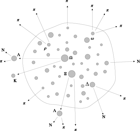
Figure 2.3: At the chemical freeze-out, the hadron gas consists of stable hadrons (with respect to strong interacions) and all hadronic resonances. The observed multiplicities obtain contributions from the primary particles (present in the fireball), and secondary particles coming from the strong decays of the resonances. In addition, the electro-weak decays should be reconstructed. In this way the yields of strange particles can be obtained.

i) Isospin Symmetry

In our approach we take into consideration all charged (isospin) states of hadrons separately. The non-zero value of the fitted chemical potential $\mu^{I}$ leads to the splitting between the multiplicities of the hadrons belonging to a given isospin multiplet. Consequently, the ratios of such hadrons may be included in our analysis. For example, we take into consideration the $\pi^{+}/\pi^{-}$ ratio measured at SPS and RHIC. The typical values of $\mu^{I}$ are of the order of 10 MeV, thus the inclusion of the isospin chemical potential represents an important effect (only at RHIC $\mu^{I}$ is practically zero).

A correct treatment of the different charged states requires that the branching ratios supplied by the Review of the Particle Physics [40] must be supplemented by the calculation of the probability of the transitions between such states. Since the strong interactions are invariant under rotations in the isospin space, the matrix elements needed for the two-body strong decays may be obtained directly from the Clebsch-Gordan coefficients. For example, we can consider the strong $\Delta\longrightarrow\pi N$ decay. Practically, this is the only decay channel of $\Delta$, so its branching ratio is 100%. In order to include different charged states of $\Delta,\,\pi$ and the nucleon, $N=(p,n)$, we combine the isospin states 1 and 1/2 into the isospin states 3/2:

$$\Delta^{++} \longrightarrow \,\left\langle 1\,1,\frac{1}{2}\,\frac{1}{2}\,|\frac{3}{2}\,\frac{3}{2}\right\rangle\,(\pi^{+}+p)=\pi^{+}+p,$$

$$\Delta^{+} \longrightarrow \,\left\langle 1\,1,\frac{1}{2}\,-\frac{1}{2}\,|\frac{3}{2}\,\frac{1}{2}\right\rangle\,\left(\pi^{+}+n\right)+\left\langle 1\,0,\frac{1}{2}\,\frac{1}{2}\,|\frac{3}{2}\,\frac{1}{2}\right\rangle\,\left(\pi^{0}+p\right)$$

$$= \frac{1}{3}\left(\pi^{+}+n\right)+\frac{2}{3}\left(\pi^{0}+p\right),$$

$$\Delta^{0} \longrightarrow \,\left\langle 1\,-1,\frac{1}{2}\,\frac{1}{2}\,|\frac{3}{2}\,-\frac{1}{2}\right\rangle\,\left(\pi^{-}+p\right)+\left\langle 1\,0,\frac{1}{2}\,-\frac{1}{2}\,|\frac{3}{2}\,-\frac{1}{2}\right\rangle\,\left(\pi^{0}+n\right)$$

$$= \frac{1}{3}\left(\pi^{-}+p\right)+\frac{2}{3}\left(\pi^{0}+n\right),$$

$$\Delta^{-} \longrightarrow \,\left\langle 1\,-1,\frac{1}{2}\,-\frac{1}{2}\,|\frac{3}{2}\,-\frac{3}{2}\right\rangle\,(\pi^{-}+n)=\pi^{-}+n.$$

ii) Experimental Branching Ratios

The case $\Delta\longrightarrow\pi N$ is very comfortable, since only a single decay channel is present and the branching ratio is obviously well known. In majority of the cases we deal with, different decay channels appear and their properties (branching ratios) are sometimes not well known. As a rule we disregard all decays with the branching ratios smaller than 1%. In addition, if the decay channels are described as dominant, large, seen, or possibly seen, we always take into account the most important channel. If two or more channels are described as equally important, we take all of them with the same weight. For example $f_{0}(980)$ decays into $\pi\pi$ (according to [40] this is the dominant channel) and $K\overline{K}$ (according to [40] this is the seen channel). In our approach, according to the rules stated above we include only the process $f_{0}(980)\longrightarrow\pi\pi$. Similarly, $a_{0}(1450)$ has three decay channels: $\eta\pi$ (seen), $\pi\eta^{\prime}(958)$ (seen), and $K\overline{K}$ (again seen). In this case we include all three decay channels with the weight (branching ratio) 1/3.

$\Delta(1600)$ decay modes	branching ratio	averaged branching ratio	rescaled branching ratio
$N\pi$	10-25 %	17.5 %	17.5 %
$N\pi\pi$	75-90 %	82.5 %	82.5 %
$\Delta\pi$	40-70 %	55.0 %	50.4 %
$N\rho$	$<$ 25 %	12.5 %	11.5 %
$N(1440)\pi$	10-35 %	22.5 %	20.6 %
$N\gamma$	0.001-0.02 %	—	—
$N\gamma,\,$helicity=1/2	0.0-0.02 %	—	—
$N\gamma,\,$helicity=3/2	0.001-0.005 %	—	—

Table 2.2: The branching ratios for the decays of $\Delta$(1600). The experimental information (second column) is averaged (third column) and rescaled (fourth column) in order to achieve the correct normalization. Similar procedure is also applied for other decays whose branching ratios are poorly known.

Another difficulty is that the branching ratios are not given exactly (instead of one value, the whole range of acceptable values is given) and the sum of the branching ratios may differ significantly from 1. In this case we take the mean values of the branching ratios. Since we require that their sum is properly normalized, sometimes we are forced to rescale all the mean values in such a way that their sum is indeed 1. To illustrate this problem we present our analysis of the decays of the $\Delta(1600)$ resonance in Table 2.2. Below, as an example we give the final branching ratios of the $\Delta(1600)^{++}$ resonance:

$$\Delta(1600)^{++} \longrightarrow 0.175\,\left(\pi^{+}+p\right)$$

$$+\,0.504\left[\,\frac{2}{5}\left(\Delta^{+}+\pi^{+}\right)+\frac{3}{5}\left(\Delta^{++}+\pi^{0}\right)\right]$$

$$+\,0.115\,\left(\,p+\rho^{+}\right)$$

$$+\,0.206\,\left[N(1400)^{+}+\pi^{+}\right].$$

We note that the correct normalization of the branching ratios is crucial for the fulfillment of the conservation laws, and consequently for the determination of the optimal thermodynamic parameters.

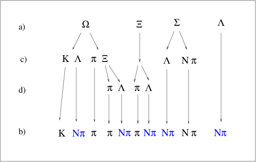
Figure 2.4: A schematic view of the weak decays of strange baryons.

iii) Weak Decays

An important part of the thermal analysis is also the correct treatment of the contributions from the electro-weak decays. For example, the final (measured) multiplicity of pions is modified by the decays of $\Lambda,\Sigma$ and $\Xi.$ Since the abundances of $\Lambda,\Sigma$ and $\Xi$ in a hot and dense matter are not negligible, their decays modify the final pion multiplicity. To study such effects, we do our calculations usually in three different ways. In the first version we include all contributions from the weak decays. In the second version we assume that there is no feedback from the weak decays – this case corresponds to the ideal situation when all weak-decay channels can be experimentally disentangled. Finally, in the third version we assume that the feedback from the weak decays is at the level of 50%. Here we follow the concept of Ref. [13].

To be more precise, in our description of the weak decays the labels $a,b,c$ and $d$ are introduced (see Fig. 2.4). The label $a$ specifies the particle multiplicity which includes the two contributions: the first one from the primordial particles, and the second one from all strong-decay channels. At the $a$-level our system includes: $\pi,\eta,K,N,\Lambda,\Sigma,\Xi$ and $\Omega$. The label $c$ characterizes the abundances corrected for the $\Omega$ and $\Sigma$ decays, whereas label $d$ means that the decays of $\Xi$ are also included. At the $d$-level we deal with: $\pi,\eta,K,N$ and $\Lambda$. The final abundances of pions, kaons and nucleons (including all electro-weak decays) are denoted by the label $b$.

iv) Resonance Mass Spectrum

In Refs. [45, 46, 47] the arguments have been presented that the mass spectra of baryons and mesons behave differently: the baryon spectrum grows more rapidly than the meson spectrum. As a consequence, the Hagedorn temperature (i.e., a scale describing the exponential growth of the spectrum) is different for baryons and mesons. With the use of a simple exponential formula, the spectra of baryons and mesons may be well parameterized as follows:

$$\rho_{B,M}(m)=A_{B,M}\exp\left[{m\over T^{B,M}_{H}}\right],$$ (2.21)

with the baryon Hagedorn temperature

$$T^{B}_{H}=186\,\hbox{MeV},$$ (2.22)

the meson Hagedorn temperature

$$T^{M}_{H}=311\,\hbox{MeV},$$ (2.23)

and the normalization constants: $A_{B}=$ 4.41 GeV and $A_{M}=$ 0.11 GeV [48].

2.3.4 Sketch of $\chi^{2}$ Method

The optimal values of the temperature $T_{chem}$ and the baryon chemical potential $\mu_{chem}^{B}$ are fitted by minimizing the expression

$$\chi^{2}=\sum_{k=1}^{n}\frac{\left(R_{k}^{\exp}-R_{k}^{therm}\right)^{2}}{\sigma_{k}^{2}},$$ (2.24)

where $R_{k}^{\exp}$ is the $k$th measured ratio, $\sigma_{k}$ is the corresponding error, and $R_{k}^{therm}$ is the same ratio determined from the thermal model. The total number of different ratios included in the analysis is denoted by $n$.

Introducing the short-hand notation $\alpha_{1}=T_{chem}$ and $\alpha_{2}=\mu_{chem}^{B}$ we may write

$$\chi^{2}\left(\alpha\right)=\chi^{2}\left(\alpha_{\min}\right)+\left(\alpha-\alpha_{\min}\right)^{T}V^{-1}\left(\alpha-\alpha_{\min}\right),$$ (2.25)

where $\alpha=\left(\alpha_{1},\alpha_{2}\right)$, $\alpha_{\min}$ is the optimal pair of the parameters, and $V$ is the variance matrix of the parameters $\alpha$. We note that $\chi^{2}\left(\alpha\right)$ has a minimum at $\alpha=\alpha_{\min}$, so the first derivatives of $\chi^{2}\left(\alpha\right)$ vanish at this point. If $F\left(\alpha\right)$ is some function of the fitted parameters $\alpha$, the variance of $F$ is given by

$$\left(\Delta F\right)^{2}=\sum_{mn}\frac{\partial F}{\partial\alpha_{m}}\frac{\partial F}{\partial\alpha_{n}}V_{mn}.$$ (2.26)

In the special cases $F=\alpha_{1}$ and $F=\alpha_{2}$ , Eq. (2.26) can be used to make an estimate of the errors of the fitted temperature and baryon chemical potential

$$\left(\Delta T_{chem}\right)^{2}=V_{11},\qquad\left(\Delta\mu_{chem}^{B}\right)^{2}=V_{22}.$$ (2.27)

Equation (2.27) will be used in our analysis with the coefficients $V_{11}$ and $V_{22}$ determined numerically.

2.3.5 Thermodynamic Characteristics of Freeze-Out

It is very interesting to know the thermodynamic properties of the hadronic matter at freeze-out. Of the particular interest is the energy density of the hadronic system. Its closeness to the critical energy density for the deconfinement phase transition (found by the Monte-Carlo simulation of QCD  on the lattice [49]) may indicate that such a phase transition indeed took place in the ultra-relativistic heavy-ion collisions. In our approach the knowledge of the temperature and the chemical potentials allows us to calculate all intensive thermodynamic quantities. In particular, we calculate the energy density

$$\varepsilon=\sum_{i}\varepsilon_{i}=\sum_{i}g_{i}\int d^{3}p\ E_{i}\left(p\right)\ f_{i}\left(p\right),$$ (2.28)

pressure

$$P=\sum_{i}P_{i}=\sum_{i}g_{i}\int d^{3}p\ \frac{p^{2}}{3\ E_{i}\left(p\right)}f_{i}\left(p\right),$$ (2.29)

and the baryon, strangeness, and isospin densities

$$\rho_{B}=\sum_{i}g_{i}\int d^{3}p\,B_{i}\,f_{i}(p),$$ (2.30)

$$\rho_{S}=\sum_{i}g_{i}\int d^{3}p\,S_{i}\,f_{i}(p),$$ (2.31)

$$\rho_{I}=\sum_{i}g_{i}\int d^{3}p\,I_{i}\,f_{i}(p).$$ (2.32)

The entropy density is determined from the Gibbs identity

$$s=\frac{\varepsilon+P-\mu_{B}\rho_{B}-\mu_{S}\rho_{S}-\mu_{I}\rho_{I}}{T}.$$ (2.33)

It is interesting to discuss the case of the classical statistics separately (this is achieved by taking the limit $\epsilon\rightarrow 0$ in the equilibrium distribution functions (2.2)). In this case the thermodynamic quantities can be expressed in terms of the modified Bessel functions

$$K_{n}(x)=\frac{2^{n}n!}{(2n)!}x^{-n}\int_{x}^{\infty}d\tau\left(\tau^{2}-x^{2}\right)^{n-1/2}e^{-\tau}.$$ (2.34)

In particular, the particle densities can be found from expression

$$n_{i}=\frac{1}{2\pi^{2}}e^{\mu_{i}/T}m_{i}^{2}TK_{2}\left(\frac{m_{i}}{T}\right),$$ (2.35)

and the corresponding energy density and the pressure are determined by the following two equations

$$\varepsilon_{i}+P_{i} = \frac{1}{2\pi^{2}}e^{\mu_{i}/T}m_{i}^{3}TK_{3}\left(\frac{m_{i}}{T}\right)$$ (2.36)

$$P_{i} = \frac{1}{2\pi^{2}}e^{\mu_{i}/T}m_{i}^{2}T^{2}K_{2}\left(\frac{m_{i}}{T}\right).$$ (2.37)

One can notice that Eqs. (2.35) and (2.37) yield the equation of state of the relativistic ideal gas of classical particles ($k_{B}=1$)

$$P=nT.$$ (2.38)

We note that it is the same as the equation of state of the non-relativistic ideal gas.

It has been pointed out by Cleymans and Redlich [14], that for a variety of different colliding systems the average energy per hadron at the chemical freeze-out is very close to 1 GeV

$$r={\varepsilon\over n}={\sum_{i}\varepsilon_{i}\over\sum_{i}n_{i}}\approx 1\,\hbox{GeV}.$$ (2.39)

In our calculations we check this relation. In addition, we calculate separately the average energy of baryons and mesons defined as

$$r_{B}={\varepsilon_{B}\over n_{B}}={\sum\limits_{baryons}\varepsilon_{i}\over\sum\limits_{baryons}n_{i}}\,\,,\hskip 28.45274ptr_{M}={\varepsilon_{M}\over n_{M}}={\sum\limits_{mesons}\varepsilon_{i}\over\sum\limits_{mesons}n_{i}}.$$ (2.40)

2.4 Modifications of Thermal Analysis

2.4.1 Finite-Size Corrections

The particle densities defined by the ideal-gas expression correspond to the thermodynamic limit, i.e., they are calculated in the limit $V\longrightarrow\infty,\,N\longrightarrow\infty$, $N/V=\,$const. In realistic situations, the hadronic systems have finite volumes and the approach based on Eq. (2.20) may be not sufficiently accurate. To include the effects of the restricted volume, one can use the modified versions of Eq. (2.20). In practice, such modifications are known only for simple geometries. In the special case of the spherical symmetry, when the hadronic system forms a fireball of radius $R_{s}$,  a correction of Eq. (2.20) may be achieved by the change of the level density [50]

$$d^{3}p\longrightarrow d^{3}p\left(1-\frac{3\pi}{4pR_{s}}+\frac{1}{(pR_{s})^{2}}+...\right).$$ (2.41)

Hence, the particle densities may be calculated from the formula

$$n_{i}=\frac{g_{i}}{2\pi^{2}}\int_{0}^{\infty}dp\left(p^{2}-\frac{3\pi p}{4R_{s}}+\frac{1}{R_{s}^{2}}+...\right)\ \left[\exp\left(\frac{E_{i}-\mu_{i,chem}}{T_{chem}}\right)+\epsilon\right]^{-1}$$ (2.42)

Clearly, for very large radii, $R_{s}\longrightarrow\infty,$ Eq. (2.42) is reduced to the standard formula (2.20). The practical calculations [9, 11] indicate that the finite-size corrections affect mainly the absolute densities. The particle ratios are not changed much due to this effect.

2.4.2 Excluded-Volume (van der Waals) Corrections

The excluded-volume corrections account for the finite volumes of hadrons. In a very dense hadronic matter the particles with finite size may overlap. This leads to strong repulsive forces and the simple approach based on Eqs. ( 2.1) and (2.2) should be modified (by definition Eqs. (2.1) and (2.2) describe non-interacting particles). Of course, the overlapping of hadrons may be the first step towards the deconfinement phase transition and creation of the quark-gluon plasma. In any case, however, the repulsive part of the nuclear force at short distances should be included in the realistic description of the hadron thermodynamics.

A fully consistent (from the thermodynamic point of view) method to include the excluded volume corrections was introduced by Yen, Gorenstein, Greiner and Yang [51]. In their approach one calculates the modified pressure $\widetilde{P}$ defined by

$$\widetilde{P}(T,\mu_{1},\mu_{2},...)=P(T,\widetilde{\mu}_{1},\widetilde{\mu}_{2},...),$$ (2.43)

where $P$ is the pressure of the ideal gas, as defined by Eq. (2.29), and $\widetilde{\mu}_{i}$ are the modified chemical potentials

$$\widetilde{\mu}_{i}=\mu_{i}-v_{i}\,\widetilde{P}(T,\mu_{1},\mu_{2},...).\quad$$ (2.44)

In Eq. (2.44) $v_{i}$ is the particle eigenvolume [51]. We note that Eq. (2.43) is a non-linear equation for $\widetilde{P}$, which can be solved by the iterative method. The particle densities $\widetilde{n}_{i}$ are the derivatives of $\widetilde{P}$ with respect to the chemical potentials $\mu_{i}$

$$\widetilde{n}_{i}\equiv\frac{\partial\widetilde{P}}{\partial\mu_{i}}=\sum_{j}\frac{\partial P}{\partial\widetilde{\mu}_{j}}\frac{\partial\widetilde{\mu}_{j}}{\partial\mu_{i}}=\sum_{j}n_{j}\left(\delta_{ji}-v_{j}\,\widetilde{n}_{i}\right),$$ (2.45)

which gives

$$\widetilde{n}_{i}(T,\mu_{i})\equiv\frac{n_{i}(T,\widetilde{\mu}_{i})}{1+\sum_{j}v_{j}\,n_{j}(T,\widetilde{\mu}_{j})}.$$ (2.46)

We observe that the modified densities are smaller than the initial densities. The reasons for this are twofold: firstly,  the denominator appearing on the right-hand side of Eq. (2.46) is always larger than one; secondly, the densities $n_{i}$ are calculated at smaller values of the chemical potential, since we have always $\widetilde{\mu}_{i}\leq\mu_{i}$.

For our investigation of the relative particle yields, it is important to realize that the denominator in Eq. (2.46) is the same for all hadron species. Hence, it cancels in the particle ratios. In addition, for the classical (Boltzmann) statistics and identical particle volumes of all hadrons ($v_{i}=v$), the modifications of the chemical potential factorize, and again cancel in the ratios. Thus, in most cases the excluded volume corrections do not affect the thermal analysis of the particle ratios and have no impact on the fitted value of the optimal temperature and baryon chemical potential

$$\frac{\widetilde{n}_{i}(T,\mu_{i})}{\widetilde{n}_{j}(T,\mu_{i})}\approx\frac{n_{i}(T,\mu_{i})}{n_{i}(T,\mu_{i})}.$$ (2.47)

Note, however, that the actual particle densities should be calculated from Eq. (2.44) with the modified chemical potential $\widetilde{\mu}_{i}$.

The case of the Boltzmann statistics is also interesting, since it leads directly to the van der Waals equation of state. To see this feature, we first write

$$\widetilde{P}=\exp\left[-\frac{v\widetilde{P}}{T}\right]P.$$ (2.48)

A derivative of Eq. (2.48) with respect to the chemical potentials yields

$$\widetilde{P}\left(1-v\widetilde{n}\right)=\widetilde{n}T,\qquad\widetilde{n}=\sum_{i}\widetilde{n}_{i},$$ (2.49)

which is a typical excluded volume correction.

2.4.3 Corrections for Undersaturation of Strangeness

The chemical equilibrium between strange and non-strange particles is more difficult to achieve because the production of $\bar{s}s$ pairs proceeds usually at a slower rate than the production of $\bar{u}u$ and $\overline{d}d$ pairs. Moreover, there are no strange quarks at the beginning of the collision process. In Ref. [12]  Rafelski has introduced an extra parameter to account for possible undersaturation of strangeness. In that approach  one calculates the hadronic densities from the formula

$$n_{i}=\frac{g_{i}}{2\pi^{2}}\int_{0}^{\infty}dpp^{2}\ \left[\gamma^{-s_{i}}\exp\left(\frac{E_{i}-\mu_{i,chem}}{T_{chem}}\right)+\epsilon\right]^{-1},$$ (2.50)

where $\gamma$ is the strangeness saturation factor ($0<\gamma\leq 1$) and $s_{i}$ is the number of valence strange quarks in the $i$th hadron.

2.5 Thermal Model in this Work

In the following Sections we apply the thermal model to describe the particle ratios measured in different experiments with ultra-relativistic heavy-ions. We use the simplest version of the model, and usually neglect the corrections discussed in Sections 2.4.1 – 2.4.3. In other words, we assume the full chemical and thermal equilibrium, and use the ideal-gas formulas. The role of the corrections defined in Sections 2.4.1 – 2.4.3 is discussed in special cases. Our method of dealing with the resonance decays was presented in detail in Section 2.3.3. The results of our calculations are denoted in the text by the label TM.

Chapter 3 Reactions with Si and S Beams

In this Chapter we use our implementation of the thermal model to analyze some of the first experiments with the ultra-relativistic heavy-ions: the experiments with the ²⁸Si beams at BNL AGS, and the experiments with ³²S beams at CERN SPS. The Alternating Gradient Synchrotron at BNL accelerated ²⁸Si ions to the energy of 14.6 GeV per nucleon (in 1986), whereas the Super Proton Synchrotron at CERN accelerated ³²S to the energy of 200 GeV per nucleon (in 1987 and later in 1990). For many years the results from sulphur-induced reactions were the main source of the data on hadron production at true ultra-relativistic energies.

3.1 Si + Au(Pb) Collisions at BNL AGS

The heavy-ion collisions with Si beams were analyzed in a thermal model by Braun-Munzinger, Stachel, Wessels, and Xu [9] (for Au and Pb targets), and later by Cleymans, Elliot, Satz, and Thews [10] (for Au targets). In this Section we are going to compare their results with our analysis of the particle ratios.

In Ref. [9] the finite-size and the excluded-volume corrections were included, and the particle ratios were calculated for two different temperatures, $T_{chem}$ = 120 MeV and $T_{chem}$ = 140 MeV, and the fixed baryon chemical potential $\mu^{B}_{chem}$ = 540 MeV. The range of temperatures considered in [9] was motivated by the experimental spectrum of the $\Delta$(1232) resonance. The value of the baryon chemical potential was constrained by the measured pion to nucleon ratio. For a given temperature and baryon chemical potential the strangeness chemical potential was adjusted to give zero net strangeness (compare Eq. (2.5)). On the other hand, the isospin chemical potential was neglected. The results of Ref. [9] are shown in Table 3.1 in the fifth (BM1) and seventh (BM2) column: one can see that the overall agreement with the data (second column) has been achieved, but the statistical significance of this result is rather poor, which is indicated by the very large values of $\chi^{2}$. In the two discussed cases one finds: $\chi^{2}/n=8.5$ and $\chi^{2}/n=12.2$.

We have reanalyzed the experimental data (as compiled in [9]) in our model assuming the full chemical equilibrium and neglecting the finite-size and excluded-volume corrections. The results of our fit are shown in the third column (TM). We have found a slightly better fit with $\chi^{2}/n=6.3$ for $T_{chem}$ = 136 MeV and $\mu^{B}_{chem}$ = 593 MeV. Still, the value of $\chi^{2}/n$ is not satisfactory. As expected, using the values of Ref. [9] for $T_{chem}$ and $\mu^{B}_{chem}$ as an input in our model (without the fitting procedure), we find the ratios corresponding to higher values of $\chi^{2}/n$. These results are shown in the fourth and sixth column denoted by TM1 and TM2, respectively. We note that our determination of the strange chemical potential agrees with the result of [9] in these two cases.

Si+Au(Pb)	experiment	TM	TM 1	BM 1	TM 2	BM 2
$T_{chem}$ [MeV]		136$\pm{\bf 2}$	120	120	140	140
$\mu_{chem}^{B}$ [MeV]		593$\pm{\bf 9}$	540	540	540	540
$\mu_{chem}^{S}$ [MeV]		152	109	108	135	135
$\mu_{chem}^{I}$ [MeV]		-14	-11	0	-13	0
$\chi^{2}/n$		6.3	9.3	8.5	22.1	12.2
$\pi/(p+n)$	1.05(5)	1.20	1.36	1.29	1.45	1.34
$\bar{p}/p$	4.5(5)$\cdot 10^{-4}$	3.6$\cdot 10^{-4}$	2.1$\cdot 10^{-4}$	1.47$\cdot 10^{-4}$	9.0$\cdot 10^{-4}$	5.8$\cdot 10^{-4}$
$K^{+}/\pi^{+}$	0.19(2)	0.23	0.23	0.23	0.24	0.27
$K^{-}/\pi^{-}$	3.5(5)$\cdot 10^{-2}$	3.3$\cdot 10^{-2}$	3.9$\cdot 10^{-2}$	5.0$\cdot 10^{-2}$	4.3$\cdot 10^{-2}$	6.2$\cdot 10^{-2}$
$K_{s}^{0}/\pi^{+}$	9.7(15)$\cdot 10^{-2}$	14$\cdot 10^{-2}$	14$\cdot 10^{-2}$	14$\cdot 10^{-2}$	15$\cdot 10^{-2}$	16$\cdot 10^{-2}$
$K^{+}/K^{-}$	4.4(4)	5.5	4.6	4.6	4.4	4.3
$\Lambda/(p+n)$	8.0(16)$\cdot 10^{-2}$	7.2$\cdot 10^{-2}$	7.6$\cdot 10^{-2}$	9.5$\cdot 10^{-2}$	8.6$\cdot 10^{-2}$	11$\cdot 10^{-2}$
$\overline{\Lambda}/\Lambda$	2.0(8)$\cdot 10^{-3}$	2.3$\cdot 10^{-3}$	1.0$\cdot 10^{-3}$	0.88$\cdot 10^{-3}$	4.4$\cdot 10^{-3}$	3.7$\cdot 10^{-3}$
$\phi/\left(K^{+}+K^{-}\right)$	1.34(36)$\cdot 10^{-2}$	2.89$\cdot 10^{-2}$	2.4$\cdot 10^{-2}$	2.4$\cdot 10^{-2}$	3.5$\cdot 10^{-2}$	3.6$\cdot 10^{-2}$
$\Xi^{-}/\Lambda$	0.12(2)	0.05	0.056	0.064	0.059	0.072

Table 3.1: Thermal analysis of the particle ratios measured in Si + Au(Pb) reactions. The experimental ratios are used in the form prepared by Braun-Munzinger et al. in Ref. [9]. The optimal values of the thermodynamic parameters found in our approach are presented in the third column (TM). The results of Ref. [9] are presented in the fifth and seventh column (denoted by BM1 and BM2, respectively). For comparison the results of our model for the same input values of $\,T_{chem}$ and $\mu^{B}_{chem}$ are shown in the fourth and sixth column (TM1 and TM2, respectively). In our calculations (TM,TM1,TM2) we include the weak decays at the level of 50%.

In Table 3.2 we show the values of the thermodynamic parameters which follow from our analysis of the particle ratios. Our best fit gives the energy density $\varepsilon$ = 0.6 GeV/fm³, and the baryon number density $\rho_{B}$ = 0.34 fm^-3 (we use here Eqs. (2.28) and (2.30)). In all considered cases the pressure satisfies the condition $P=(n_{M}+n_{B})\,T$, which indicates that the matter at the chemical freeze-out behaves like an ideal classical gas (compare Eq. (2.38)). In this situation the excluded-volume corrections cancel in the particle ratios and do not affect the optimal values of the temperature and the baryon chemical potential (as discussed in the end of Section 2.4.2). The classical form of the equation of state is a consequence of the fact that most of the particles included in the thermal approach are heavy resonances, which are well described by the classical distribution functions. The important role of heavy resonances in the thermal analysis is reflected also by the fact that the final density of pions (resulting from the decays of resonances) is much higher than the primordial density. Initially, the pion density is 0.09 fm^-3. With the inclusion of the strong decays of the resonances, the pion density increases up to 0.35 fm^-3. We also note that the contribution from the decays of the $\rho$-mesons to the final pion density is at the level of 15%. This means that most of the extra pions is produced by the decays of heavier resonances. The last raw in Table 3.2 shows the Cleymans-Redlich ratio calculated for three different choices of $T_{chem}$ and $\mu^{B}_{chem}$. In all cases we observe that $r\approx$ 1 GeV. It is interesting to notice, however, that $r_{B}$ is significantly larger than $r_{M}$. This feature reflects a different behavior of the mass spectra of baryons and mesons, as displayed by Eqs. (2.21) - (2.23).

Si+Au(Pb)	TM	TM 1	TM 2
$T_{chem}$ [MeV]	136	120	140
$\mu_{chem}^{B}$ [MeV]	593	540	540
$\mu_{chem}^{S}$ [MeV]	152	109	135
$\mu_{chem}^{I}$ [MeV]	-14	-11	-13
$\varepsilon_{B}$ [GeV/fm3]	0.48	0.14	0.42
$\varepsilon_{M}$ [GeV/fm3]	0.12	0.05	0.14
$\varepsilon$ [GeV/fm3]	0.60	0.19	0.56
$P$ [GeV/fm3]	0.07	0.02	0.07
$\rho_{B}$ [1/fm3]	0.34	0.11	0.29
$s$ [1/fm3]	3.4	1.3	3.3
$n_{B}$ [1/fm3]	0.34	0.11	0.29
$n_{M}$ [1/fm3]	0.17	0.09	0.19
$r_{B}$ [GeV]	1.4	1.3	1.4
$r_{M}$ [GeV]	0.7	0.6	0.7
$r$ [GeV]	1.2	1.0	1.1

Table 3.2: Thermodynamic parameters at the chemical freeze-out, as inferred from the analysis of the particle ratios in the Si+Au(Pb) collisions at AGS. The results correspond to the Table 3.1, where the fitted ratios are shown.

The large values of $\chi^{2}/n$, shown in Table 3.1, indicate that thermal description of the particle yields does not work well for reactions with the silicon beams. Even the ratio of pions to nucleons does not come out accurately, giving quite large contribution to $\chi^{2}/n$. In the thermal analysis of Ref. [9] the isospin chemical potential is zero, so the ratios such as $\pi^{+}/p\,\,$ or $\pi^{-}/p$ are necessarily the same. The experimental estimate of Ref. [9] for any of these ratios is $(2/3)\,\pi/(p+n)=(2/3)\,1.05\approx 0.7$. This result was updated in Ref. [10], where the collisions with Au targets are included only, and the following values are used: $\pi^{+}/p=0.8$ and $\pi^{-}/p=1.0$. The approach of Ref. [10] has the non-zero isospin chemical potential, so differences in the abundances of the states belonging to the same isospin multiplets can be easily included. In addition, the authors of Ref. [10] decided to apply the thermal model to the particle species which are most abundant. Consequently, their fit includes only five ratios: $\pi^{+}/p,\,K^{+}/\pi^{+},\,K^{+}/K^{-},\,\Lambda/p$ and $K^{-}/\pi^{-}$. Note, that the ratio $\pi^{-}/p$ is not independent and it is not included in the calculation.

The results of the thermal fit of Ref. [10] are presented in Table 3.3 in the last column denoted by CEST. The experimental data in the second column are taken also from Ref. [10]. We have run our code and obtained the results shown in the third column denoted by TM. First of all, we see that the five ratios included in the analysis are quite well reproduced in the thermal model ($\chi^{2}/n\approx 0.5$). Our calculation fully confirms the result of Ref. [10] which gives: $T_{chem}=110$ MeV and $\mu^{B}_{chem}=540$ MeV. The four remaining ratios of less abundant hadron species are treated in this case as an output of the thermal model. They are shown in the four bottom raws of Table 3.3. Naturally, the agreement of the model in this case is not as good as for the five “input” ratios.

Si+Au	experiment	TM	CEST
$T_{chem}$ [MeV]		108$\pm{\bf 5}$	110$\pm{\bf 5}$
$\mu_{chem}^{B}$ [MeV]		540$\pm{\bf 10}$	540$\pm{\bf 20}$
$\mu_{chem}^{S}$ [MeV]		93
$\mu_{chem}^{I}$ [MeV]		-9
$\chi^{2}/n\,(n=5)$		0.5	0.6
$\pi^{+}/p$	0.80$\pm 0.08$	0.84	0.87
$K^{+}/\pi^{+}$	0.19$\pm 0.02$	0.20	0.21
$K^{+}/K^{-}$	4.40$\pm 0.40$	4.50	4.51
$\Lambda/p$	0.20$\pm 0.04$	0.14	0.16
$K^{-}/\pi^{-}$	0.035$\pm 0.005$	0.035	0.038
$\Xi^{-}/\Lambda$	(1.2$\pm 0.2$)$\cdot 10^{-1}$	5.2$\cdot 10^{-2}$	4.9$\cdot 10^{-2}$
$\phi/\pi^{+}$	(4.5$\pm 1.2$)$\cdot 10^{-3}$	4.2$\cdot 10^{-3}$	4.6$\cdot 10^{-3}$
$\bar{p}/p$	(4.5$\pm 0.4$)$\cdot 10^{-4}$	7.2$\cdot 10^{-5}$	7.2$\cdot 10^{-5}$
$\overline{\Lambda}/\Lambda$	(2.0$\pm 0.8$)$\cdot 10^{-3}$	3.2$\cdot 10^{-4}$	3.4$\cdot 10^{-4}$

Table 3.3: Thermal-model analysis of the particle ratios for Si + Au collisions. The experimental data are taken from the paper by Cleymans et al., see Ref. [10]. The results of Ref. [10] are given in the last column (CEST) and compared to our calculation (TM). In the calculation of $\chi^{2}$ only five ratios of the most abundant hadron species are included: $\pi^{+}/p,\,K^{+}/\pi^{+},\,K^{+}/K^{-},\,\Lambda/p$ and $K^{-}/\pi^{-}$. The remaining four ratios (the bottom four raws) are treated here as an output of the thermal model. In our calculation the weak decays were included again at the 50% level.

In Table 3.4 we show the result of the thermal analysis obtained in the case when all nine ratios are included in the calculation of $\chi^{2}$. Our calculation gives $T_{chem}=127$ MeV and $\mu^{B}_{chem}=533$ MeV. As expected, the quality of the fit, $\chi^{2}/n\approx 3$, is worse than that obtained in the previous case with only five ratios included. On the other hand, it is better than the quality of the fits presented in Table 3.1 for Si + Au(Pb) collisions. The better agreement is caused by the use of the updated ratios of pions to nucleons in Ref. [10], which are more consistent with the thermal picture.

Si+Au	experiment	TM	CEST
$T_{chem}$ [MeV]		127$\pm{\bf 3}$	110$\pm{\bf 5}$
$\mu_{chem}^{B}$ [MeV]		533$\pm{\bf 13}$	540$\pm{\bf 20}$
$\mu_{chem}^{S}$ [MeV]		116
$\mu_{chem}^{I}$ [MeV]		-11
$\chi^{2}/n\,(n=9)$		3.1	12.2
$\pi^{+}/p$	0.80$\pm 0.08$	0.87	0.87
$K^{+}/\pi^{+}$	0.19$\pm 0.02$	0.23	0.21
$K^{+}/K^{-}$	4.40$\pm 0.40$	4.42	4.51
$\Lambda/p$	0.20$\pm 0.04$	0.17	0.16
$K^{-}/\pi^{-}$	0.035$\pm 0.005$	0.042	0.038
$\Xi^{-}/\Lambda$	(1.2$\pm 0.2$)$\cdot 10^{-1}$	5.8$\cdot 10^{-2}$	4.9$\cdot 10^{-2}$
$\phi/\pi^{+}$	(4.5$\pm 1.2$)$\cdot 10^{-3}$	8.2$\cdot 10^{-3}$	4.6$\cdot 10^{-3}$
$\bar{p}/p$	(4.5$\pm 0.4$)$\cdot 10^{-4}$	4.1$\cdot 10^{-4}$	7.2$\cdot 10^{-5}$
$\overline{\Lambda}/\Lambda$	(2.0$\pm 0.8$)$\cdot 10^{-3}$	1.9$\cdot 10^{-3}$	3.4$\cdot 10^{-4}$

Table 3.4: Thermal-model analysis of the particle ratios for Si + Au collisions. The experimental data are taken from [10]. In this case, our calculation (TM) includes all 9 ratios in the construction of $\chi^{2}$. The last column repeats the results of Cleymans et al., see Table 3.3, which were obtained by fitting only the first 5 ratios. The value of $\chi^{2}/n$ is calculated in both cases (TM and CEST) for all 9 ratios.

S + Au(W,Pb)	experiment	TM	TM 1	BM 1	TM 2	BM 2
$T_{chem}$ [MeV]		179$\pm{\bf 2}$	160	160	170	170
$\mu_{chem}^{B}$ [MeV]		199$\pm{\bf 4}$	170	170	180	180
$\mu_{chem}^{S}$ [MeV]		55	37	38	45	47
$\mu_{chem}^{I}$ [MeV]		-7	-4	0	-5	0
$\chi^{2}/n$		4.2	11.3	7.7	5.6	6.6
$K_{s\ b}^{0}/\Lambda_{d}$	0.88(10)	1.29	1.68	1.57	1.46	1.36
$K_{s\ b}^{0}/\overline{\Lambda}_{d}$	4.6(10)	5.4	7.8	7.3	6.15	5.7
$\overline{\Lambda}_{c}/\Lambda_{c}$	0.20(1)	0.21	0.19	0.20	0.21	0.23
$\overline{\Lambda}_{d}/\Lambda_{d}$	0.19(4)	0.24	0.21	0.22	0.24	0.24
$\Xi_{c}^{-}/\Lambda_{c}$	0.095(6)	0.112	0.12	0.12	0.16	0.12
$\Xi_{c}^{+}/\overline{\Lambda}_{c}$	0.21(2)	0.20	0.18	0.20	0.19	0.21
$p/\pi^{+}$	0.18(3)	0.29	0.22	0.17	0.25	0.19
$(h^{+}-h^{-})/h^{-}$	0.15(1)	0.19	0.14	0.18	0.16	0.21
$\left(p-\bar{p}\right)/h^{-}$	0.15(2)	0.20	0.15	0.13	0.17	0.14
$\left(h^{+}-h^{-}\right)/\left(h^{+}+h^{-}\right)$	0.088(7)	0.085	0.067	0.084	0.075	0.094
$\bar{p}/p$	0.12(2)	0.14	0.14	0.13	0.15	0.14
$\bar{p}/\pi^{-}$	0.024(9)	0.037	0.029	0.022	0.035	0.027
$\eta/\pi^{0}$	0.15(2)	0.11	0.12	0.12	0.11	0.12
$\phi/\left(\rho+\omega\right)$	0.080(20)	0.055	0.053	0.11	0.055	0.12
$(K^{+}+K^{-})/(2K_{s}^{0})$	1.07(3)	1.03	1.03	1.05	1.03	1.06
$K^{+}/K^{-}$	1.67(15)	1.58	1.44	1.46	1.49	1.53
$K_{s}^{0}/\Lambda$	1.4(1)	1.6	2.12	1.74	1.84	1.50
$K_{s}^{0}/\overline{\Lambda}$	6.4(4)	7.1	10.3	8.5	8.1	6.6
$\Lambda/(p-\bar{p})$	0.45(4)	0.43	0.44	0.67	0.45	0.69
$\overline{\Lambda}/\bar{p}$	0.80(30)	0.62	0.55	0.38	0.59	0.41
$\overline{\Lambda}/\Lambda$	0.207(12)	0.226	0.206	0.20	0.226	0.23
$\Xi^{-}/\Lambda$	0.066(13)	0.114	0.120	0.12	0.118	0.12
$\Xi^{+}/\overline{\Lambda}$	0.127(22)	0.185	0.172	0.20	0.178	0.21
$\Xi^{+}/\Xi^{-}$   (WA85)	0.45(5)	0.37	0.30	0.31	0.34	0.36
$\Xi^{+}/\Xi^{-}$   (NA36)	0.276(108)	0.37	0.30	0.31	0.34	0.36
$\frac{\left(\Omega^{+}+\Omega^{-}\right)}{\left(\Xi^{+}+\Xi^{-}\right)}$	0.8(4)	0.2	0.2	0.17	0.18	0.19

Table 3.5: Thermal analysis of the particle ratios measured in S + Au(W,Pb) reactions. The experimental ratios are taken from Ref. [11]. The optimal values of the thermodynamic parameters found in our approach are presented in the third column (TM). The results of Ref. [11] are presented in the fifth and seventh column (denoted by BM1 and BM2, respectively). For comparison the results of our model for the same input values of $\,T_{chem}$ and $\mu^{B}_{chem}$ are shown in the fourth and sixth column (TM1 and TM2, respectively). Except for the first six measured ratios (where the weak decays have been disentangled), we include the weak decays at the level of 50%.

3.2 S + Au(W,Pb) Collisions at CERN SPS

The thermal analysis of the S + Au(W,Pb) collisions was performed by Braun-Munzinger, Stachel, Wessels, and Xu in Ref. [11]. In Table 3.5 we show their results (BM1, BM2) together with our analysis based on the assumption of the full chemical and thermal equilibrium (TM, TM1, TM2). In our approach we have again neglected the finite-size and the excluded-volume corrections. The presentation of the results in Table 3.5 is analogous to that given in Table 3.1. We see again that the values of $\chi^{2}/n$ are quite large, indicating that the thermal model describes the measured ratios only in a qualitative way.

In Table 3.6 we give the values of the thermodynamic parameters at the freeze-out. They exhibit similar features to those found in the case of the Si + Au collisions discussed in the previous Section. In particular, we observe the classical equation of state, quite large energy density and baryon number density, different Cleymans-Redlich ratios for mesons and baryons.

S + Au(W,Pb)	TM	TM 1	TM 2
$T_{chem}$ [MeV]	179$\pm 2$	160	170
$\mu_{chem}^{B}$ [MeV]	199$\pm 4$	170	180
$\mu_{chem}^{S}$ [MeV]	55	37	45
$\mu_{chem}^{I}$ [MeV]	-7	-4	-5
$\varepsilon_{B}$ [GeV/fm3]	0.44	0.15	0.26
$\varepsilon_{M}$ [GeV/fm3]	0.64	0.30	0.45
$\varepsilon$ [GeV/fm3]	1.1	0.45	0.71
$P$ [GeV/fm3]	0.16	0.07	0.11
$\rho_{B}$ [1/fm3]	0.20	0.07	0.12
$s$ [1/fm3]	6.7	3.1	4.7
$n_{B}$ [1/fm3]	0.27	0.09	0.16
$n_{M}$ [1/fm3]	0.65	0.35	0.49
$r_{B}$ [GeV]	1.6	1.6	1.6
$r_{M}$ [GeV]	1.0	0.8	0.9
$r$ [GeV]	1.2	1.0	1.1

Table 3.6: Thermodynamic parameters at the chemical freeze-out, as inferred from the analysis of the particle ratios in the S+Au(W,Pb) collisions at SPS. The results correspond to the cases described in Table 3.5.

3.3 Concluding Remarks

Thermal analysis of the particle ratios measured in the collisions of relatively lighter nuclei, such as Si or S, leads only to a qualitative agreement with the data. This may indicate that the produced systems are not in the full chemical equilibrium, or they are too small for the thermodynamic concepts to be applicable. It is also possible that the errors of the experimentally determined ratios are underestimated (the true systematic errors may be larger, note the discrepancy seen in the measurement of the $\Xi^{+}/\Xi^{-}$ ratio done by different groups). Our calculations based on the $\chi^{2}$ method agree well with the results of Ref. [10], where only a limited number of the particle ratios was studied. On the other hand, we observe appreciable differences between our fits and the global parametrization of the data proposed in Refs. [9, 11].

Chapter 4 Pb + Pb Collisions at CERN SPS

Lead on lead collisions at 158 GeV per nucleon were the first really heavy -ion collisions at fully relativistic energies. In this case we dealt, for the first time, with large volumes and life-times of the reaction region. Simple estimates based on the Bjorken hydrodynamic model [34] indicate that matter with the energy density of a few GeV/fm³ was created at the early stage of the central collisions. Such energy density exceeds the critical energy density for the phase transition from a hadron gas to a quark-gluon plasma [49], so the transient existence of the plasma could occur in these reactions [52].

In the first part of this Chapter we show the results of the thermal analysis of the particle ratios, which is based on our own implementation of the thermal model. Subsequently, we discuss the impact of the possible in-medium modifications of hadron masses and widths on the thermal fits.

4.1 Thermal Analysis of Particle Ratios

Pb+Pb	experiment	max. feeding	no feeding	50% feeding
$T_{chem}$ [MeV]		164$\pm{\bf 3}$	170$\pm{\bf 3}$	168$\pm{\bf 3}$
$\mu_{chem}^{B}$ [MeV]		234$\pm{\bf 7}$	250$\pm{\bf 8}$	244$\pm{\bf 8}$
$\mu_{chem}^{S}$ [MeV]		56	65	62
$\mu_{chem}^{I}$ [MeV]		-8	-9	-9
$\chi^{2}/n$		1.4	1.8	0.9
$\left(p_{a}-\overline{p}_{a}\right)/h_{a}^{-}$	0.228(29)	0.209	0.233	0.224
$\overline{p}_{a}/p_{a}$	0.055(10)	0.062	0.058	0.060
$\overline{p}_{b}/p_{b}$	0.085(8)	0.083	0.080	0.081
$\overline{\Lambda}_{c}/\Lambda_{c}$	0.131(17)	0.118	0.118	0.118
$\Xi_{c}^{-}/\Lambda_{c}$	0.110(10)	0.107	0.104	0.105
$\Xi_{c}^{+}/\overline{\Lambda}_{c}$	0.206(40)	0.202	0.210	0.207
$\pi^{-}/\pi^{+}$	1.1(1)	1.2	1.1	1.1
$\eta/\pi^{0}$	0.081(13)	0.099	0.121	0.109
$K_{S\ }^{0}/\pi^{-}$	0.125(19)	0.149	0.172	0.159
$K_{S\ }^{0}/h^{-}$	0.123(20)	0.131	0.149	0.138
$\Lambda/h^{-}$	0.077(11)	0.102	0.076	0.091
$\Lambda/K_{S}^{0}$	0.63(8)	0.78	0.51	0.66
$K^{+}/K^{-}$    (NA44)	1.85(9)	1.68	1.78	1.74
$K^{+}/K^{-}$    (NA49)	1.8(1)	1.68	1.78	1.74
$\Xi^{+}/\overline{\Lambda}$	0.188(39)	0.142	0.291	0.191
$\frac{\left(\Xi^{+}+\Xi^{-}\right)}{\left(\Lambda+\overline{\Lambda}\right)}$	0.13(3)	0.09	0.16	0.12
$\Xi^{+}/\Xi^{-}$       (NA49)	0.232(33)	0.223	0.237	0.232
$\Xi^{+}/\Xi^{-}$       (WA97)	0.247(43)	0.223	0.237	0.232
$\Omega^{+}/\Omega^{-}$	0.383(81)	0.448	0.522	0.493
$\Omega^{-}/\Xi^{-}$	0.219(45)	0.133	0.136	0.135

Table 4.1: Thermal-model results for the particle ratios measured in Pb+Pb collisions at CERN SPS. The experimental data are used in the form compiled in Ref. [13]. The contribution from the weak decays is treated in three different ways: i)maximal feeding (third column) means that the contributions from all weak decays are included in the multiplicities of the produced hadrons, ii) no feeding (fourth column) means that the weak decays have been reconstructed, and the contributions from the weak decays are not included, and iii) 50% feeding means that 50% of the contribution from the weak decays is included in the final multiplicities.

With the same implementation of the thermal model as that used in the previous Chapter to describe the collisions of lighter nuclei, we have studied the particle ratios measured for Pb + Pb collisions at 158 GeV per nucleon. We have used the data in the form compiled by Braun-Munzinger, Heppe, and Stachel in Ref. [13]. The authors of Ref. [13] argued that the particle ratios can be well described in the framework of the thermal model. Our calculations support this point of view – our fits to the particle ratios are shown in Table 4.1. To check the validity of our results, we did our calculations in three different ways, treating differently contributions from the weak decays. The three methods were introduced in the end of Section 2.3.3 (see also Fig. 2.4 where a scheme of the weak decays is presented). The first 6 ratios listed in Table 4.1 were measured in such a way that the feedback from the weak decays was well established. Consequently, these ratios enter in the same way the three versions of our calculation. The remaining 14 ratios are treated differently in each case. For example, the $\Lambda/h^{-}$ ratio equals: $\Lambda_{d}/h_{b}^{-}$ in the first version (maximal feeding, shown in the third column), $\Lambda_{a}/h_{a}^{-}$ in the second version (no feeding, the fourth column), and $\left(\Lambda_{a}+\Lambda_{d}\right)/\left(h_{a}^{-}+h_{b}^{-}\right)$ in the third version (averaged feeding, the fifth column). Other ratios are treated in the similar way. In the second column the experimental data are shown according to Ref. [13]. We observe that different treatment of the weak-decay contributions leads to slightly different values of $T_{chem},\mu_{chem}^{B},\mu_{chem}^{S}$ and $\mu_{chem}^{I}$, but the three cases are consistent with each other within errors (compare the first two raws of Table 4.1).

The best fit is obtained when the feeding from the weak decays is averaged, which corresponds most likely to the experimental situation. In this case: $T_{chem}=168\pm 3$ MeV and $\mu_{chem}^{B}=244\pm 8$ MeV. The authors of Ref. [13] obtained $T_{chem}=168\pm 2$ MeV and $\mu_{chem}^{B}=266\pm 5$ MeV. The agreement of the fitted temperatures is very good, the difference of the fitted values of the baryon chemical potential may be caused by a different treatment of many branching ratios which are not well known. In the most realistic case (50% feeding) our $\chi^{2}$ per one degree of freedom is smaller than one, indicating a good quality of the thermal fit, see Fig. 4.1 where the contour plot of $\chi^{2}/n$ is shown. The total number of degrees of freedom is 20 in our case. It is smaller by one from the number of ratios included in Ref. [11], since we discard the deuteron measurement. The latter may be disturbed by the inclusion of nuclear fragments.

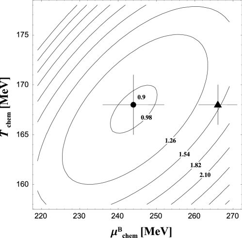
Figure 4.1: The contour plot of $\chi^{2}/n$ for the ratios measured in Pb+Pb collisions at CERN SPS. The numbers at the contours give our values of $\chi^{2}/n$. Our optimal values of $T_{chem}$ and $\mu^{B}_{chem}$ are denoted by the black circle. The optimal values of Ref. [13] are denoted by the triangle. The crosses mark the errors.

Pb+Pb	experiment	quantum statistics	classical statistics	$m<$ 1.8 GeV	$m\leq m_{\Omega}$
$T_{chem}$ [MeV]		168$\pm{\bf 3}$	167$\pm{\bf 3}$	171$\pm{\bf 3}$	171$\pm{\bf 3}$
$\mu_{chem}^{B}$ [MeV]		244$\pm{\bf 8}$	243$\pm{\bf 8}$	247$\pm{\bf 8}$	248$\pm{\bf 8}$
$\mu_{chem}^{S}$ [MeV]		62	62	62	61
$\mu_{chem}^{I}$ [MeV]		-9	-9	-9	-8
$\chi^{2}/n$		0.9	1.1	0.9	1.1
$\left(p_{a}-\overline{p}_{a}\right)/h_{a}^{-}$	0.228(29)	0.224	0.228	0.228	0.212
$\overline{p}_{a}/p_{a}$	0.055(10)	0.060	0.060	0.061	0.060
$\overline{p}_{b}/p_{b}$	0.085(8)	0.081	0.081	0.082	0.083
$\overline{\Lambda}_{c}/\Lambda_{c}$	0.131(17)	0.118	0.118	0.118	0.117
$\Xi_{c}^{-}/\Lambda_{c}$	0.110(10)	0.105	0.105	0.115	0.123
$\Xi_{c}^{+}/\overline{\Lambda}_{c}$	0.206(40)	0.207	0.207	0.229	0.240
$\pi^{-}/\pi^{+}$	1.1(1)	1.1	1.1	1.1	1.1
$\eta/\pi^{0}$	0.081(13)	0.109	0.111	0.109	0.114
$K_{S\ }^{0}/\pi^{-}$	0.125(19)	0.159	0.162	0.156	0.161
$K_{S\ }^{0}/h^{-}$	0.123(20)	0.138	0.140	0.136	0.140
$\Lambda/h^{-}$	0.077(11)	0.091	0.093	0.090	0.092
$\Lambda/K_{S}^{0}$	0.63(8)	0.66	0.66	0.67	0.66
$K^{+}/K^{-}$   (NA44)	1.85(9)	1.74	1.73	1.76	1.78
$K^{+}/K^{-}$   (NA49)	1.8(1)	1.74	1.73	1.76	1.78
$\Xi^{+}/\overline{\Lambda}$	0.188(39)	0.191	0.192	0.208	0.217
$\frac{\left(\Xi^{+}+\Xi^{-}\right)}{\left(\Lambda+\overline{\Lambda}\right)}$	0.13(3)	0.12	0.12	0.13	0.14
$\Xi^{+}/\Xi^{-}$      (NA49)	0.232(33)	0.232	0.233	0.231	0.226
$\Xi^{+}/\Xi^{-}$      (WA97)	0.247(43)	0.232	0.233	0.231	0.226
$\Omega^{+}/\Omega^{-}$	0.383(81)	0.493	0.498	0.486	0.471
$\Omega^{-}/\Xi^{-}$	0.219(45)	0.135	0.134	0.140	0.141

Table 4.2: Thermal-model results for the particle ratios measured in Pb+Pb collisions at CERN SPS. The experimental data are taken from Ref. [13]. The role of the quantum statistics and the mass cut is displayed.

4.2 Sensitivity to Classical Statistics and Limited Mass Spectrum

In this Section, we discuss the sensitivity of our results to two different modifications. The first modification is simply a replacement of the quantum distribution functions by the classical distributions (the Bose-Einstein distribution for mesons and the Fermi-Dirac distribution for baryons are replaced by the Boltzmann distribution for all hadrons including pions and kaons). The second modification is connected with the introduction of a limiting hadron mass. In this way we can check how important the tail of the mass distribution of hadrons is for the results of our analysis.

The results obtained with the classical distribution functions and with the limited hadron mass spectrum are shown in Table 4.2. The data are listed in the second column. In the third column we present our results obtained for exact quantum statistics. They coincide with the last column of Table 4.1, i.e., we average the feeding from the weak decays here. In the fourth column we show the results for the classical statistics. The fifth and sixth columns show our results obtained with the limited mass spectrum. In the fifth column we neglect the feedback from the resonances heavier than 1.8 GeV, whereas in the sixth column the maximal mass is equal to the mass of $\ \Omega$ ($m_{\Omega}=$ 1.672 GeV). In each column we show the corresponding values of the optimal thermodynamic parameters and $\chi^{2}/n$.

We find that the use of the classical distribution functions leads to very small changes of our results. The values of $T_{chem}$ and $\mu^{B}_{chem}$ change only by 1 MeV, and $\chi^{2}/n$ increases from 0.9 to 1.1. The quantum statistics are not important in the thermal analysis because most of particles are very heavy and they can be described well by the classical distributions. Even for pions we can use the classical statistics, since they are produced mainly by the decays of heavier resonances. The classical features of the hadronic fireball at the freeze-out are also reflected in the equation of state, which has a form $P=(n_{M}+n_{B})T$. Cutting the mass spectrum at 1.8 GeV changes the values of $T_{chem}$ and $\mu^{B}_{chem}$ by 3 MeV. The cut at $m_{\Omega}=$ 1.672 GeV has a similar impact on $T_{chem}$ and $\mu^{B}_{chem}$, which remain in agreement (within errors) with the exact results. We have checked that the cuts at smaller masses, $\sim 1.6$ GeV, cause already appreciable changes of $T_{chem}$ and $\mu^{B}_{chem}$.

4.3 Thermodynamic Properties of Freeze-Out

In this Section we present the complete set of the thermodynamic parameters characterizing the chemical freeze-out in Pb + Pb collisions at CERN SPS. We have again done our calculations in three different ways, treating differently contributions from the weak decays. As discussed above, in the three considered cases the values of $T_{chem}$ and $\mu^{B}_{chem}$ are consistent with each other. It is interesting to observe, however, that small differences in $T_{chem}$ and $\mu^{B}_{chem}$ may result in quite large changes of other thermodynamic parameters, obtained as the integrals over the distribution functions (2.2). In Table 4.3 we show the energy density, pressure, baryon number density, entropy, baryon and meson densities, and the Cleymans-Redlich ratios. We find that different treatment of the weak decays causes that the thermal-model estimate of the energy density at the chemical freeze-out varies from 0.6 GeV/fm³ to 0.8 GeV/fm³. Similarly, the baryon density at the freeze-out changes from 0.13 fm^-3 to 0.19 fm^-3. Such changes indicate, that the correct experimental reconstruction of the weak decays is necessary in order to have more precise information about the state of matter at the freeze-out. The last three raws of Table 4.3 show the Cleymans-Redlich ratio calculated for baryons ($r_{B}$), mesons ($r_{M}$), and all hadrons ($r$). We observe that $r$ is close to unity in the three considered cases, i.e., it is insensitive to the way in which the weak decays are treated. We again find that $r_{B}$ is much larger than $r_{M}$.

Pb+Pb	Max. feeding	No feeding	50 %  feeding
$T_{chem}$ [MeV]	164$\pm 3$	170$\pm 3$	168$\pm 3$
$\mu_{chem}^{B}$ [MeV]	234$\pm 7$	250$\pm 8$	244$\pm 8$
$\mu_{chem}^{S}$ [MeV]	56	65	62
$\mu_{chem}^{I}$ [MeV]	-8	-9	-9
$\varepsilon_{B}$ [GeV/fm3]	0.24	0.35	0.31
$\varepsilon_{M}$ [GeV/fm3]	0.35	0.45	0.41
$\varepsilon$ [GeV/fm3]	0.59	0.80	0.72
$P$ [GeV/fm3]	0.09	0.12	0.11
$\rho_{B}$ [1/fm3]	0.13	0.19	0.17
$s$ [1/fm3]	4.0	5.1	4.7
$n_{B}$ [1/fm3]	0.15	0.22	0.19
$n_{M}$ [1/fm3]	0.40	0.49	0.46
$r_{B}$ [GeV]	1.6	1.6	1.6
$r_{M}$ [GeV]	0.9	0.9	0.9
$r$ [GeV]	1.1	1.1	1.1

Table 4.3: Thermodynamic parameters at the chemical freeze-out in Pb + Pb collisions at CERN SPS. Different treatment of the weak decays leads to quite large changes in the estimates of the energy density, baryon number density, and other thermodynamic quantities.

4.4 Scaling of Masses and Widths at Freeze-Out

Thermal-model fits show that the temperature at the chemical freeze-out, $T_{chem}$, as well as the baryon density, are large. As we have just seen in the previous Sections, one typically obtains $T_{chem}\sim$ 170 MeV, which is close to the expected critical value for the deconfinement/hadronization phase transition [49]. In this situation one may expect that hadron properties at the chemical freeze-out are strongly modified by the presence of the hadronic environment. Indeed, such modifications are predicted by different model calculations $[28-31]$, which helps to explain the low-mass dilepton enhancement observed in the CERES [53] and HELIOS [54] experiments. In this Section we incorporate possible modifications of hadron masses and widths into thermal analysis of the particle ratios. We generalize the results of Refs. [43, 44] where the problem was studied without refitting thermodynamic parameters.

Initially, we include only the mass modifications and calculate the particle densities from the ideal-gas expression

$$n_{i}=\frac{g_{i}}{2\pi^{2}}\int_{0}^{\infty}\frac{p^{2}\ dp}{\exp\left[\left(E_{i}^{\ast}-\mu_{chem}^{B}B_{i}-\mu_{chem}^{S}S_{i}-\mu_{chem}^{I}I_{i}\right)/T_{chem}\right]+\epsilon}\,,$$ (4.1)

where

$$E_{i}^{\ast}=\sqrt{p^{2}+\left(m_{i}^{\ast}\right)^{2}}$$ (4.2)

is the energy. Of course, in standard thermal-model fits Eq. (4.1) is used with the vacuum masses, $m_{i}^{\ast}=m_{i}$. The in-medium masses, $m_{i}^{\ast}$, may depend on temperature and density in a complicated way. In order to explore possible different behavior of in-medium masses and, at the same time, keep simplicity, we do our calculations with the meson and baryon masses rescaled by the two universal parameters, $x_{M}$ and $x_{B}$, namely

$$m_{M}^{\ast}=x_{M}\,m_{M},\hskip 14.22636ptm_{B}^{\ast}=x_{B}\,m_{B}.$$ (4.3)

An exception from this rule are the masses of pseudo-Goldstone bosons ($\pi$, $K$, $\eta$) which we keep constant. This is in agreement with explicit model calculations incorporating chiral symmetry, e.g. [55, 56]. We note that the use of Eq. (4.1) is valid when the in-medium hadrons can be regarded as good quasi-particles. A thermodynamically consistent approach has been constructed so far only for the lowest multiplets of hadrons [41]. At SPS energies, however, it is crucial to include all hadrons with masses up to (at least) 1.6 GeV. For such a complicated system, a thermodynamically consistent approach is not available. As in the standard approach, Eq. (4.1) is used to calculate the primordial density of stable hadrons and resonances at the chemical freeze-out. The final (observed) multiplicities receive contributions from the primordial stable hadrons, and from the secondary hadrons produced by decays of resonances after the freeze-out. Ref. [40] is used to determine the branching ratios, which we keep unchanged. We neglect the finite-size and excluded volume corrections which do not affect the particle ratios.

For fixed values of $x_{M}$ and $x_{B}$ we fit the temperature, $T_{chem}$, and the baryonic chemical potential, $\mu_{chem}^{B}$, by the minimization the expression

$$\chi^{2}(x_{M},x_{B})=\sum\limits_{k=1}^{n}{\left[R_{k}^{\,exp}-R_{k}^{\,therm}(x_{M},x_{B})\right]^{2}\over\sigma_{k}^{2}},$$ (4.4)

where $R_{k}^{\,exp}$ is the $k$th measured ratio, $\sigma_{k}$ is the corresponding error, and $R_{k}^{\,therm}(x_{M},x_{B})$ is the same ratio as determined from the thermal model with the modified masses. Similarly to the standard case with unchanged masses, $m_{i}^{*}=m_{i}$, the strange chemical potential, $\mu_{chem}^{S},$ and the isospin chemical potential, $\mu_{chem}^{I}$, are determined from the requirements that the initial strangeness of the system is zero, and that the ratio of the baryon number to the electric charge is the same as in the colliding nuclei, see Eqs. (2.5) and (2.6).

Figure 4.2: Dependence of $\chi^{2}$, and the fitted values of the temperature and the baryon density on the scale parameter $x$. Plot represents Pb + Pb collisions at SPS energies. Solid lines: all hadron masses (except for Goldstone bosons) are scaled with $x_{M}=x_{B}=x$. Dashed line: only meson masses are scaled, $x_{M}=x,x_{B}=1$. Dotted lines: only baryon masses are scaled, $x_{B}=x,x_{M}=1$. The nuclear saturation density $\rho_{0}$ = 0.17 fm^-3.

In Fig. 4.2 we plot our results obtained for the experimental ratios measured in Pb + Pb collisions at SPS. In the case $x_{M}=x_{B}=1$ we recover our results discussed in detail in Sections 4.1 – 4.3. In Fig. 4.2 a) we give our values of $\chi^{2}$. One can observe that a small decrease of the meson and baryon masses, $x_{M}=x_{B}\sim 0.9$, leads to a slightly better fit with the corresponding smaller values of the temperature and the baryon density, as shown in Figs. 4.2 b) and 4.2 c). It would be premature, however, to conclude that the masses drop. The values of $\chi^{2}$ for the solid line are increased by 25% compared to the minimum in the range $0.75<x<1.05$, which clearly is the allowed range. We thus conclude that moderate dropping of hadron masses, say by 20%, does not spoil the quality of thermal fits. On the contrary, larger dropping or growing of the masses result in a significant increase of the $\chi^{2}$ values.

With the modified masses the thermodynamic parameters characterizing the fits change. For example, if we rescale both meson and baryon masses (except for Goldstone bosons) in the same way, $x=x_{M}=x_{B}$, the temperature and the chemical potentials  are to a very good approximation also rescaled by $x$. This follows from the fact that we study a system of equations which is invariant under rescaling of all quantities with the dimension of energy. If we allowed also for the changes of the masses of the Goldstone bosons, the thermodynamic parameters would scale exactly as $T_{chem}(x)=x\ T_{chem}(x=0)$ and $\mu_{chem}(x)=x\ \mu_{chem}(x=0)$. In this case $\chi^{2}$ remains constant, independently of $x$. For fixed values of the Goldstone-boson masses, the scale invariance is broken, $\chi^{2}$ varies with $x$, as shown in Fig. 4.2 a), and the results are non-trivial.

To account for finite in-medium widths, $\Gamma_{i}^{\ast}$, of the resonances we generalize Eq. (4.1) to the formula [57-60]

$$n_{i}=\int\limits_{M_{0}^{2}}^{\infty}dM^{2}\int\limits_{0}^{\infty}dp\,\,{\frac{1}{\pi N}}{\frac{m_{i}^{\ast}\Gamma_{i}^{\ast}}{(M^{2}-(m_{i}^{\ast})^{2})^{2}+(m_{i}^{\ast}\Gamma_{i}^{\ast})^{2}}}$$

$$\times\frac{g_{i}}{2\pi^{2}}\frac{p^{2}}{\exp\left[\left(\sqrt{M^{2}+p^{2}}-\mu_{chem}^{B}B_{i}-\mu_{chem}^{S}S_{i}-\mu_{chem}^{I}I_{i}\right)/T_{chem}\right]\pm 1},$$ (4.5)

where $N$ is the normalization of the relativistic Breit-Wigner function,

$$N={\frac{1}{2}}+{\frac{1}{\pi}}\arctan\left[((m_{i}^{\ast})^{2}-M_{0}^{2})/(m_{i}^{\ast}\Gamma_{i}^{\ast})\right]\approx 1.$$ (4.6)

The integral over $M^{2}$ is taken to start at the threshold $M_{0}^{2}$ corresponding to the dominant decay channel. In the limit $\Gamma_{i}^{\ast}\rightarrow 0$ Eq. (4.5) obviously reduces to formula (4.1).

In order to analyze the effect of broadening of hadron widths we introduce the parameter $y$ in such a way that

$$\Gamma_{i}^{\ast}=y\,\Gamma_{i}.$$ (4.7)

Here $\Gamma_{i}$ are the vacuum widths, hence the case $y=1$ corresponds to the physical widths as measured in the vacuum, and the case $y=0$ represents the situation when the widths are neglected (our previous analysis based on Eq. (4.1)). In Fig. 4.3 we show the results of our fitting procedure. We observe that the inclusion of the vacuum widths does not change the value of $\chi^{2}$, and the values of $T_{chem}$ and $\rho_{chem}^{B}$. An increase of the widths by a factor of 2 has also little effect. Only for larger modifications of the widths the fit gets worse.

In conclusion we state that the thermal analysis of particle ratios, measured in Pb + Pb collisions at CERN SPS, allows for moderate dropping of hadron masses ($\sim$ 20%). This does not spoil the fits, which remain of similar quality as those obtained without modifications. Larger dropping of the hadron masses or growing of the masses are not likely. Scaling of hadron masses results in modifications of the thermodynamic parameters for which the fits are optimal. In particular, lowering of  all the masses leads to a smaller values of $T_{chem}$ and $\rho_{chem}^{B}$. This might be a desired effect, since $T_{chem}\sim$170 MeV is large and may correspond to quark-gluon plasma rather than to a hadron gas. Our study of the modifications of the hadron widths shows that they have small impact on the ratios.

Figure 4.3: Dependence of $\chi^{2}$, and the optimal values of the temperature and the baryon density on the scale parameter for the widths, $y$.

Chapter 5 Au + Au Collisions at BNL RHIC

The heavy-ion program at CERN SPS delivered several very interesting results, but there was no clear discovery of the new physical phenomena, such as the desired deconfinement phase transition. The newest heavy-ion machine, the Relativistic Heavy-Ion Collider constructed at BNL, was designed to accelerate heavy ions at energy $\sqrt{s}=$ 200 GeV. In the year 2000, during the first run of RHIC, the maximal energy of $\sqrt{s}=$ 130 GeV was achieved. This energy exceeds the CERN SPS energy by one order of magnitude , so the new phenomena were expected to occur. The first new RHIC data indicate indeed at several new features of the collision process such as: much higher particle multiplicities, increased production of antiparticles, and lower baryon number in the central region. Nevertheless, the overall picture of the collision follows the pattern established from the studies of heavy-ion collisions at lower energies. Further systematic analysis of the just incoming data is necessary to extract more information.

5.1 Thermal Analysis of Particle Ratios

Table 5.1 presents our fit to the particle ratios measured at RHIC during its first run at $\sqrt{s}=$ 130 GeV. We stress that exactly the same version of the thermal model has been used in this fit, as that used in our previous studies of Si + Au, S + Au, and Pb + Pb reactions. In our present calculation, the identical ratios measured by different groups are treated separately in the definition of $\chi^{2}$ (number of points $n=16$). In this way the measurements done by different groups enter independently, and converging experimental data have a larger weight in the statistical analysis. Very similar results are obtained, however, if we first average the results of different groups to obtain the most likely value for each considered ratio. This fact shows consistency of the experimental measurements done by different groups, see the third column in Table 5.1.

Our optimal value of $T_{chem}$ obtained from the analysis of the particle ratios equals $165\pm 7$ MeV. It is a very interesting fact that $T_{chem}$ for RHIC agrees well with $T_{chem}=168\pm 3$ MeV found in our fit for Pb + Pb collisions at CERN SPS. The growth of the energy of the colliding nuclei by one order of magnitude does not lead to creation of a hotter system, only the baryon chemical potential is significantly lower than that found at CERN SPS. Clearly, the collisions at RHIC energies are more transparent than the collisions at CERN energies. We have also calculated other characteristics of the freeze-out. In particular, we find the energy density $\varepsilon=0.5$ GeV/fm³, the pressure $P=$ 0.08 GeV/fm³, and the baryon density $\rho_{B}=$ 0.02 fm^-3. Here again, one can observe that the energy density is not higher than that found at CERN SPS, only the net baryon number tends rapidly to zero. Our calculation confirms the Cleymans-Redlich conjecture [14] that the energy per hadron at the chemical freeze-out is 1 GeV (our approach yields almost exactly $r=$ 1.0 GeV). We observe, however, that the average baryon energy is much larger than the average meson energy: $r_{B}=$ 1.6 GeV and $r_{M}=$ 0.9 GeV. We emphasize that exactly the same $r_{B}$ and $r_{M}$ have been extracted from Pb + Pb collisions at CERN SPS, see Table 4.3. Also the values of $r_{B}$ and $r_{M}$ extracted from the sulphur collisions, see Table 3.6, agree well with these two values. Further work is needed to explain such universal behavior. In addition, in our thermal approach we find that the ratios $\overline{\Lambda}/\Lambda$ and $\overline{\Xi}/\Xi$ are practically unaffected by the weak decays, since the latter contribute in the same way to the abundances of baryons and antibaryons (note the very small value of our $\mu^{B}_{chem}$).

Au+Au	TM	experiment
$T_{chem}$ [MeV]	165$\pm{\bf 7}$
$\mu_{chem}^{B}$ [MeV]	41$\pm{\bf 5}$
$\mu_{chem}^{S}$ [MeV]	9
$\mu_{chem}^{I}$ [MeV]	-1
$\chi^{2}/n$	0.97
$\pi^{-}/\pi^{+}$	$1.02$	$1.00\pm 0.02$ [61], $0.99\pm 0.02$[62]
$\overline{p}/\pi^{-}$	$0.09$	$0.08\pm 0.01$ [63]
$K^{-}/K^{+}$	$0.92$	$0.88\pm 0.05$ [64], $0.78\pm 0.12$ [65] $0.91\pm 0.09$ [61], $0.92\pm 0.06$ [62]
$K^{-}/\pi^{-}$	$0.16$	$0.15\pm 0.02$ [64]
$K_{0}^{\ast}/h^{-}$	$0.046$	$0.060\pm 0.012$ [64, 66]
$\overline{K_{0}^{\ast}}/h^{-}$	$0.041$	$0.058\pm 0.012$ [64, 66]
$\overline{p}/p$	$0.65$	$0.61\pm 0.07$ [63], $0.54\pm 0.08$ [65] $0.60\pm 0.07$ [61], $0.61\pm 0.06$ [62]
$\overline{\Lambda}/\Lambda$	$0.69$	$0.73\pm 0.03$ [64]
$\overline{\Xi}/\Xi$	$0.76$	$0.82\pm 0.08$ [64]

Table 5.1: Thermal fit of the particle ratios measured at RHIC at $\sqrt{s}=130$ GeV.

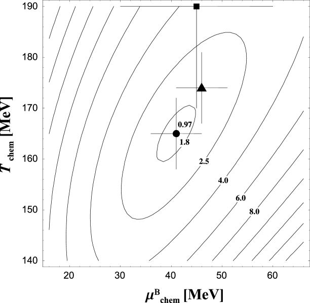
Figure 5.1: The contour plot of our $\chi^{2}/n$. Our result (black circle), the result of Ref. [19] (black square), and the fit of Ref. [20] (black triangle) are all shown with the corresponding errors. The numbers at the contours indicate the values of $\chi^{2}/n$.

In Fig. 5.1 we show $\chi^{2}/n$ as a function of the temperature, $T_{chem}$, and the baryon chemical potential, $\mu^{B}_{chem}$. An interesting feature of the plot is that it shows a characteristic valley of the optimal values of the thermodynamic parameters. The shape of this valley indicates that the quality of the fit does not change much if we moderately increase or decrease both $T_{chem}$ and $\mu^{B}_{chem}$. We note that a similar valley can be seen in Fig. 4.1, where the values of $\chi^{2}/n$ were plotted for the case of Pb + Pb collisions at CERN SPS. While our work was nearing completion [21], a fit by Braun-Munzinger, Magestro, Redlich and Stachel was presented: $T_{chem}=174\pm 7$ MeV and $\mu^{B}_{chem}=46\pm 5$ MeV [20]. We note that our $T_{chem}$ is 9 MeV lower than $T_{chem}$ of Ref. [20], and 25 MeV lower than 190 MeV obtained in a similar fit by Xu and Kaneta [19]. Still, the results of the three calculations are consistent within errors. This fact is displayed in Fig. 5.1, where our result (black circle), the fit of Ref. [20] (black triangle), and the fit of Ref. [19] (black square) are shown all together with the corresponding errors. Especially, the results of Refs. [20] and [21] are close and line up along the valley of the optimal parameters.

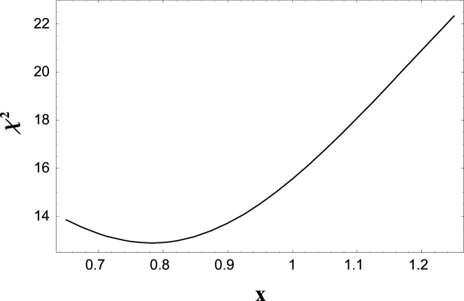
Figure 5.2: Dependence of $\chi^{2}$ on the scale parameter $x$. In this case $x_{B}=x_{M}=x$, i.e., the masses of baryons and mesons are rescaled in the same way (except for the pseudo-Goldstone bosons).

Similarly to the case of Pb + Pb collisions at CERN SPS, we have studied the influence of possible in-medium mass modifications on the thermal analysis of the ratios measured at RHIC. In Fig. 5.2 we show the dependence of $\chi^{2}$ on the scale parameter $x$ (in this case the mass modifications of baryons and mesons are assumed to be equal). We observe that the values of $\chi^{2}$ are slightly lowered for $x<1$. This is analogous behavior to that observed in Pb + Pb collisions studied in Sect. 4.4. Again, the effect is not dramatic ($\chi^{2}$ decreases by 20% if $x$ changes from 1 to 0.8), so the indication for dropping masses is rather weak. On the other hand, we see that the changes of the masses can be included in the thermal analysis, yielding the fits of the same quality as that found in the calculations without any modifications. In the present case, however, we see that larger dropping of the masses is allowed, as compared to the CERN-SPS case discussed before. We have also analyzed Si + Au collisions at AGS, and S + Au collisions at SPS. In these two cases $\chi^{2}$ has a flat minimum at $x_{M}\approx x_{B}\approx 1$.

5.2 Pressure of Hadron Gas at Freeze-Out

In Fig. 5.3 we plot the pressure of a hadron gas as a function of the temperature and the baryon chemical potential. We show the neighborhood of the optimal parameters: $T_{chem}=165$ MeV and $\mu^{B}_{chem}=41$ MeV. The exact result shown in Fig. 5.3, obtained as a sum of all partial pressures given by Eq. (2.29), can be very well approximated by the formula

$$P_{HG}(T,\mu^{B}) = {1\over 2\pi^{2}}\int\limits_{0}^{M_{\max}}\rho_{M}(m)\,m^{2}\,T^{2}\,K_{2}\left({m\over T}\right)\,dm$$ (5.1)

$$+{1\over\pi^{2}}\int\limits_{0}^{M_{\max}}\rho_{B}(m)\,\hbox{cosh}\left({\mu^{B}\over T}\right)m^{2}\,T^{2}\,K_{2}\left({m\over T}\right)\,dm$$

$$= {1\over 2\pi^{2}}\int\limits_{0}^{M_{\max}}\left[\rho_{M}(m)+2\,\hbox{cosh}\left({\mu^{B}\over T}\right)\rho_{B}(m)\right]m^{2}\,T^{2}\,K_{2}\left({m\over T}\right)\,dm.$$

In Eq. (5.1) the sum over all hadronic states is replaced by the convolution of the classical formula for the partial pressure, Eq. (2.37), with the mass spectrum for baryons and mesons, Eqs. (2.22) and (2.23). The maximal mass included in the integral is taken to be the same as that used in the fits of the spectrum [47], $M_{\max}=1.8$ GeV. We note that the strange chemical potential as well as the isospin chemical potential have been neglected in Eq. (5.1). Our fit shows that these two potential are very small at RHIC. For $T=165$ MeV and $\mu^{B}=41$ MeV, the pressure calculated from Eq. (5.1) agrees very well with the exact result $P=0.08$ GeV/fm³. The very weak dependence of the pressure on the baryon chemical potential, as displayed in Fig. 5.3, follows also from Eq. (5.1), since in the considered region one finds $\hbox{cosh\,}(\mu^{B}/T)\approx 1$.

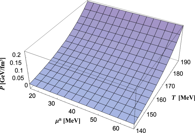
Figure 5.3: Pressure of a hadron gas which includes all resonances consisting of up, down, and strange quarks.

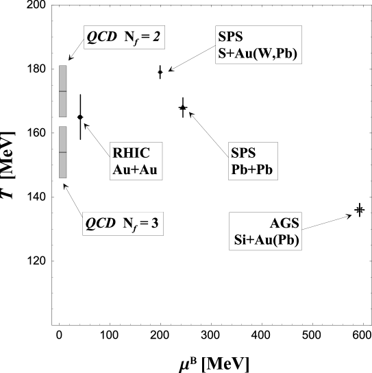
Figure 5.4: Our optimal thermodynamic parameters. The fitted values of the temperature for Pb + Pb collisions at CERN SPS and for Au + Au collisions at BNL RHIC are consistent with each other, and close to the critical temperature predicted by the QCD simulations on a lattice [49]. The lattice results (grey bands) correspond to two different versions of the calculations (the number of massless flavors, $N_{f}$, is taken to be either 2 or 3). The vertical size of the bands denotes the error of the lattice calculations. We show also our optimal parameters describing the collisions of lighter nuclei. Note that in this case the quality of the fits is worse, as discussed in detail in Chapter 3.

It is constructive to compare the pressure of the hadron gas at freeze-out to the pressure of the ideal gas of quarks and gluons at the same temperature and baryon chemical potential. To do so we use the formula

$$P_{QGP}(T,\mu_{q})={1\over 3}\left[16{\pi^{2}\over 30}T^{4}+6N_{f}\left({7\pi^{2}\over 120}T^{4}+{1\over 4}\mu^{2}_{q}T^{2}+{1\over 8\pi^{2}}\mu^{4}_{q}\right)\right]-B,$$ (5.2)

where $N_{f}$ is the number of quark flavors and $B$ is the bag constant. For $T=165$ MeV, $\mu_{q}=\mu^{B}/3=41/3$ MeV (the quark chemical potential is one third of the baryon chemical potential), $B^{1/4}=$ 200 MeV, and $N_{f}=3$ one finds $P=0.3$ GeV/fm³. This result shows that the pressure of the ideal gas of quarks and gluons is much larger than the pressure of a hadron gas (we recall that our calculation gives $P=0.08$ GeV/fm³). If the equation of state (5.2) was realistic, we would deal with the plasma rather than with a hadron gas at the temperatures as high as $T=165$ MeV. More realistic equations of state of the plasma include interactions of quarks and gluons which lower the pressure of the plasma and increase the temperature of the possible phase transition. The most reliable predictions concerning the phase transition are obtained by the numerical studies of QCD on a discretized space-time lattice [49]. The most recent values of the critical temperature are: $T_{c}=173\pm 8$ MeV for $N_{f}=2$, and $T_{c}=154\pm 8$ MeV for $N_{f}=3$. It is intriguing that the thermal fits of the particle ratios yield the temperature, which is very close to the critical temperature inferred from the lattice simulations. The closeness of these two temperatures suggests that the chemical content of the hadronic fireball is established just after hadronization phase transition or, some authors argue, during the hadronization process itself. In the latter case the thermal distributions of hadrons have little in common with rescattering. Note, however, that our fit is consistent (within errors) with a temperature smaller than $T_{c}$.

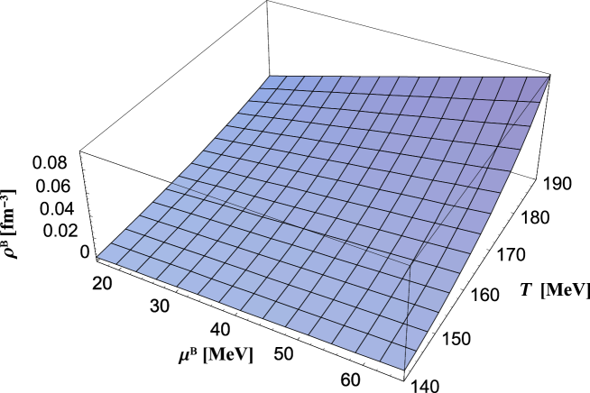
Figure 5.5: Baryon density of a hadron gas in the vicinity of the freeze-out point: $T_{chem}=165$ MeV and $\mu^{B}_{chem}=41$ MeV.

We close this Section with the two additional plots. In Fig. 5.5 we show the baryon density of a hadron gas in the region close to our optimal thermodynamic parameters. In the considered region the baryon density is very low. It is much smaller than the baryon saturation density $\rho_{0}=0.17$ fm^-3 (we note that for Pb + Pb collisions at CERN SPS the fitted baryon density was close to $\rho_{0}$). Finally, in Fig. 5.6 we plot the Cleymans-Redlich ratio. One can observe that $r$ is close to unity ($0.8<r<1.2$) in the rather vast range of the temperature and the baryon chemical potential.

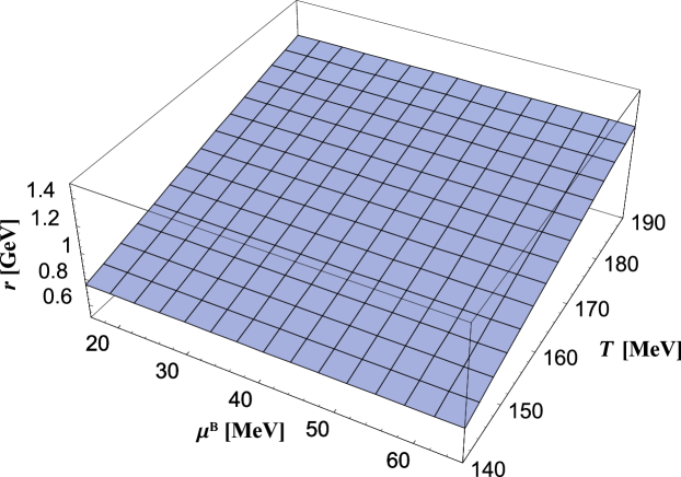
Figure 5.6: Cleymans-Redlich ratio for a hadron gas.

Chapter 6 Conclusions

In the end of the paper we summarize the main findings of our work:

• Thermal description of the particle ratios, based on the assumption of the full chemical and thermal equilibrium, works well for Pb + Pb collisions at CERN SPS and Au + Au collisions at BNL RHIC. At smaller beam energies and for smaller sizes of the colliding systems this version of the thermal model reproduces only a qualitative behavior of the data. We stress that this observation follows from the study which uses exactly the same framework for all reactions.

• The optimal values of the temperature inferred from the thermal analysis of the ratios in Pb + Pb collisions at CERN SPS and Au + Au collisions at BNL RHIC agree. The more energetic collisions at RHIC do not produce a hotter hadronic system. The fitted value of the temperature ($T_{chem}\sim 165$ MeV for RHIC and $T_{chem}\sim 168$ MeV for SPS), is very close to the critical temperature obtained from the lattice simulations of QCD.

• In the case of Pb + Pb collisions at CERN SPS energies, the correct reconstruction of the weak decays is essential for the estimates of the energy density and the baryon number density characterizing the freeze-out. On the other hand, at RHIC the role of the weak decays is less important.

• Our calculations confirm the Cleymans-Redlich observation that thermal conditions at freeze-out, for different colliding systems at different energies, correspond to an average hadron energy 1 GeV. Moreover, we have found that averaged baryon energy is 1.6 GeV and the average meson energy is 0.9 GeV for both Pb + Pb collisions at CERN SPS and Au + Au collisions at BNL RHIC. This new observation is parallel to the argument that two different Hagedorn temperatures are required to describe the mass spectra of baryons and mesons.

• Possible modifications of the hadron masses and widths were incorporated into a thermal analysis of the particle ratios. In the case of Pb + Pb collisions at CERN SPS, we have found that moderate, up to 20%, dropping of the masses does not spoil the quality of the fits. Larger dropping or growing of the masses are not likely, since they result in a significant increase of the $\chi^{2}$ values. We have also showed that the increase of hadron widths by less than a factor of two does not affect the thermal-model fits. Similar behavior is found for Au + Au collisions at BNL RHIC. In this case, however, larger dropping of the masses is allowed.

• We have checked, for a variety of colliding systems, that the quantum statistics (Bose-Einstein and Fermi-Dirac) can be very well approximated by the classical Boltzmann statistics. This means that the hadron gas at the freeze-out behaves like a classical gas with the equation of state $P=nT$. In addition, the use of the Boltzmann distribution function implies that the excluded-volume corrections do not change the values of the fitted optimal values of $T_{chem}$ and $\mu^{B}_{chem}$ (provided the eigenvolumes of baryons and mesons are equal).

• Finally, we emphasize that our fits may be treated as a first step in more complex investigations of hadron production in ultra-relativistic heavy-ion collisions. A combination of the thermal approach with the hydrodynamic expansion can be used to study other observables such as: transverse-momentum spectra, rapidity distributions, elliptic flow, or HBT correlation radii.

ACKNOWLEDGMENTS

I would like to thank Dr. Wojciech Florkowski for suggesting this investigation, stimulating remarks, and numerous discussions concerning the problems presented in this dissertation.

I am also grateful to Dr. Wojciech Broniowski for his interest in this study, critical comments, and encouragement.

I would like to thank Prof. Edward Kapuścik for his help and guidance during my PhD studies, and Prof. Jan Kwieciński for his interest in this work. I thank also my colleagues from the Theory Department of the Institute of Nuclear Physics for interesting discussions.

Finally, I would like to thank my family, especially my wife Kinga, for their understanding, patience and support.

Bibliography

High-Energy Nuclear Collisions
- [1] QUARK MATTER ’90. Proceedings, 8th International Conference on Ultra-Relativistic Nucleus-Nucleus Collisions, MENTON, FRANCE, Nucl. Phys. A525 (1991)
- [2] QUARK MATTER ’91. Proceedings, 9th International Conference on Ultra-Relativistic Nucleus-Nucleus Collisions, GATLINBURG, USA, Nucl. Phys. A544 (1992)
- [3] QUARK MATTER ’93. Proceedings, 10th International Conference on Ultra-Relativistic Nucleus-Nucleus Collisions, BORLÄNGE, SWEDEN, Nucl. Phys. A566 (1994)
- [4] QUARK MATTER ’95. Proceedings, 11th International Conference on Ultra-Relativistic Nucleus-Nucleus Collisions, MONTEREY, USA, Nucl. Phys. A590 (1995)
- [5] QUARK MATTER ’96. Proceedings, 12th International Conference on Ultra-Relativistic Nucleus-Nucleus Collisions, HEIDELBERG, GERMANY, Nucl. Phys. A610 (1996)
- [6] QUARK MATTER ’97. Proceedings, 13th International Conference on Ultra-Relativistic Nucleus-Nucleus Collisions, TSUKUBA, JAPAN, Nucl. Phys. A638 (1998)
- [7] QUARK MATTER ’99. Proceedings, 14th International Conference on Ultra-Relativistic Nucleus-Nucleus Collisions, TORINO, ITALY, Nucl. Phys. A661 (1999)
- [8] QUARK MATTER ’01. Proceedings, 15th International Conference on Ultra-Relativistic Nucleus-Nucleus Collisions, Brookhaven National Laboratory, USA, Nucl. Phys. A in print Thermal Models
- [9] P. Braun-Munzinger, J. Stachel, J. P. Wessels, and N. Xu, Phys. Lett. B344 (1995) 43
- [10] J. Cleymans, D. Elliott, H. Satz, and R. L. Thews, Z. Phys. C74 (1997) 319
- [11] P. Braun-Munzinger, J. Stachel, J. P. Wessels, and N. Xu, Phys. Lett. B365 (1996) 1
- [12] J. Rafelski, J. Letessier, and A. Tounsi, Acta Phys. Pol. B28 (1997) 2841
- [13] P. Braun-Munzinger, I. Heppe, and J. Stachel, Phys. Lett. B465 (1999) 15
- [14] J. Cleymans and K. Redlich, Phys. Rev. Lett. 81 (1998) 5284
- [15] G. D. Yen and M. I. Gorenstein, Phys. Rev. C59 (1999) 2788
- [16] F. Becattini, J. Cleymans, A. Keranen, E. Suhonen, and K. Redlich, Phys. Rev. C64 (2001) 024901
- [17] F. Becattini, J. Cleymans, A. Keranen, E. Suhonen, and K. Redlich, hep-ph/0011322
- [18] M. Gaździcki, Nucl. Phys. A681 (2001) 153
- [19] N. Xu and M. Kaneta, nucl-ex/0104021, Proceedings of QM2001, Nucl. Phys. A in print
- [20] P. Braun-Munzinger, D. Magestro, K. Redlich, and J. Stachel, Phys. Lett. B518 (2001) 41
- [21] W. Florkowski, W. Broniowski, and M. Michalec, nucl-th/0106009
- [22] J. Rafelski and J. Letessier, Phys. Rev. Lett. 85 (2000) 4695
- [23] W. Broniowski and W. Florkowski, nucl-th/0106050, Phys. Rev. Lett. in print Models of QGP Production
- [24] A. Bialas, W. Czyż, A. Dyrek, and W. Florkowski, Nucl. Phys. B296 (1988) 611; A. Dyrek and W. Florkowski, Nuovo Cim. 102A (1989) 1013
- [25] K. Geiger, Phys. Rep. 258 (1995) 237 Hadrons in Medium
- [26] Hadrons in Nuclear Matter, Proceedings of the International Workshop XXIII on Gross Properties of Nuclei and Nuclear Excitations, Hirschegg, AUSTRIA, 1995
- [27] Hadrons in Dense Matter, Proceedings of the International Workshop XXVIII on Gross Properties of Nuclei and Nuclear Excitations, Hirschegg, AUSTRIA, 2000
- [28] T. Hatsuda, H. Shiomi, and H. Kuwabara, Prog. Theor. Phys. 95 (1996) 1009
- [29] F. Klingl, N. Kaiser, and W. Weise, Nucl. Phys. A624 (1997) 527
- [30] T. Hatsuda and S. H. Lee, Phys. Rev. C46 (1992) R34
- [31] G. Brown and M. Rho, Phys. Rev. Lett. 66 (1991) 2720 Relativistic Hydrodynamics
- [32] E. Fermi, Prog. Theor. Phys. 5 (1950) 570; Phys. Rev. 92 (1953) 452
- [33] L.D. Landau, Izv. Akad. Nauk SSSR, Ser. Fiz., 17 (1953) 51, also published in “Collected papers of L.D. Landau”, ed. by D. Ter Haar, Pergamon Press (1965) 569
- [34] J. Bjorken, Phys. Rev. D27 (1983) 140
- [35] G. Baym, B. Friman, J.-P. Blaizot, M. Soyeur and W. Czyż, Nucl. Phys. A407 (1983) 541
- [36] U. Heinz, J. Phys. G25 (1999) 263
- [37] J. Cleymans, H. Oeschler, and K. Redlich, J. Phys. G25 (1999) 281
- [38] F. Cooper, G. Frye, Phys. Rev. D10 (1974) 186
- [39] F. Cooper, G. Frye, and E. Schonberg, Phys. Rev. D11 (1975) 192 Particle Data Tables
- [40] Particle Data Group, Eur. Phys. J. C15 (2000) 1 Modifications of Hadron Properties at Freeze-Out
- [41] D. Zschiesche, L. Gerland, S. Schramm, J. Schaffner-Bielich, H. Stoecker, and W. Greiner, Nucl. Phys. A681 (2001) 34
- [42] M. Michalec, W. Florkowski, and W. Broniowski, Phys. Lett. B520 (2001) 213
- [43] W. Florkowski, W. Broniowski, Phys. Lett. B477 (2000) 73
- [44] W. Florkowski and W. Broniowski, Proceedings of the International Workshop XXVIII on Gross Properties of Nuclei and Nuclear Excitations, Hirschegg, AUSTRIA, 2000, p. 275 Hagedorn Temperature
- [45] W. Broniowski and W. Florkowski, Phys. Lett. B490 (2000) 223
- [46] W. Broniowski, Few-Quark Problems, Proceedings of the Mini-Workshop, Bled, Slovenia, 2000, p. 14
- [47] W. Broniowski, Acta Phys. Pol. B31 (2000) 2155
- [48] W. Broniowski, private communication Lattice QCD
- [49] F. Karsch, hep-ph/0103314, Proceedings of QM2001, Nucl. Phys. A in print Finite-Size and Excluded-Volume Corrections
- [50] H. R. Jaqama, A. Z. Mekijan, and L. Zamick, Phys. Rev. C29 (1984) 2067, see also R. Balian and C. Bloch, Ann. Phys. 70 (1970) 401
- [51] G. D. Yen, M. I. Gorenstein, W. Greiner, S.-N. Yang, Phys. Rev. C56 (1997) 2210 CERN Press Release Feb. 10, 2000
- [52] http://cern.web.cern.ch/CERN/Announcements/2000/NewStateMatter/ Experiments on Dilepton Production
- [53] CERES Collab., G. Agakichiev et al., Phys. Rev. Lett. 75 (1995) 1272
- [54] HELIOS/3 Collab., M. Masera et al., Nucl. Phys. A590 (1995) 93c Chiral Models at Finite Temperature/Density
- [55] M. Lutz, S. Klimt, and W. Weise, Nucl. Phys. A542 (1992) 521; M. Lutz, A. Steiner, and W. Weise, Nucl. Phys. A574 (1994) 755
- [56] T. Hatsuda and T. Kunihiro, Phys. Rep. 247 (1994) 221, and references therein Thermodynamics of Hadron Gas
- [57] E. Beth and G. E. Uhlenbeck, Physica 3 (1936) 729; Physica 4 (1937) 915
- [58] R. Dashen, S.-K. Ma and H. J. Bernstein, Phys. Rev. 187 (1969) 345
- [59] W. Weinhold, Zur Thermodynamik des N-Systems, Diplomarbeit, GSI, Sept. 1995
- [60] W. Weinhold, B. Friman, and W. Norenberg, Acta Phys. Pol. B27 (1996) 3249; Phys. Lett. B433 (1998) 236 Experimental Results for RHIC
- [61] B. B. Back et al., PHOBOS Collaboration, Phys. Rev. Lett. 85 (2000) 3100
- [62] I. G. Bearden, BRAHMS Collaboration, Proceedings of QM2001, Nucl. Phys. A in print
- [63] J. Harris, STAR Collaboration, Proceedings of QM2001, Nucl. Phys. A in print
- [64] H. Caines, STAR Collaboration, Proceedings of QM2001, Nucl. Phys. A in print
- [65] H. Ohnishi, PHENIX Collaboration, Proceedings of QM2001, Nucl. Phys. A in print
- [66] Z. Xu, nucl-ex/0104001, Proceedings of QM2001, Nucl. Phys. A in print