Strange particle production at RHIC in a single-freeze-out model [1]

Abstract

Strange particle ratios and $p_{\perp}$-spectra are calculated in a thermal model with single freeze-out, previously used successfully to describe non-strange particle production at RHIC. The model and the recently released data for $\phi$, $\Lambda$, $\overline{\Lambda}$ and $K^{*}(892)^{0}$ are in very satisfactory agreement, showing that the thermal approach can be used to describe the strangeness production at RHIC.

I Introduction

In this paper we calculate the ratios and the $p_{\perp}$-spectra for the strange particles produced at RHIC at $\sqrt{s}=130$ GeV A. We use the thermal model with single freeze-out. The work is a direct follow-up of our previous study reported in Ref. [2]. The very recent data from the STAR collaboration on the production of $\phi$ [3], $\Lambda$ [4], $\overline{\Lambda}$ [4], and $K^{*}(892)^{0}$ [5] are confronted with the model and a very good agreement is found.

Enhanced strangeness production in the high-energy nuclear collisions, relative to more elementary $pp$ or $e^{+}e^{-}$ collisions, was proposed many years ago [6, 7] as a signal of the quark-gluon plasma formation (for more recent arguments and discussion see, e.g., [8]). In the meantime, the experimental evidence for the enhancement has indeed been found, however its significance for the plasma formation remains an open problem [9]. The ratios of the particle abundances measured in Pb+Pb collisions at SPS ($\sqrt{s}=$17 GeV A) and in Au+Au collisions at RHIC ($\sqrt{s}=$130 GeV A) are very well explained in the framework of the thermal models which use the hadronic degrees of freedom only [10, 11, 12]. In this approach one assumes that the net strangeness is zero, and the strange hadrons are in a complete thermal and chemical equilibrium with other hadrons. A combination of the thermal model with a suitable hydrodynamic expansion (the single-freeze-out model of Ref. [2]) led to a very good quantitative description of the RHIC transverse-momentum spectra of pions, kaons, and protons. In this paper we present the predictions of this model for the production of other particles, with a special emphasis on the strangeness production. Without any refitting of the two thermal and two expansion parameters of Ref. [2], we calculate the $p_{\perp}$-spectra of $\phi$, $\Lambda$, $\overline{\Lambda}$, $K^{*}(892)^{0}$, $\Xi$, $\Sigma$, and $\Omega$. The spectra of $\phi$, $\Lambda$, $\overline{\Lambda}$ and $K^{*}(892)^{0}$ are in a very good agreement with the very recently released data [3, 4, 5]. The spectra of other particles are also presented and will be confronted with the incoming future data. We also compute the thermal spectrum of the $J/\psi$.

II Definition of the model

The main assumption of our model is that the chemical freeze-out occurs simultaneously with the thermal freeze-out, i.e., the hadrons decouple completely when the thermodynamic parameters reach the freeze-out conditions. In other words, the possible elastic rescattering processes after the chemical freeze-out are neglected. This assumption opposes the most popular scenario [13], where the two freeze-outs are separated. The argument used in this context is the difference of scales, following from the fact that the elastic cross sections are, for most channels, much larger than the inelastic cross sections (note, however, that this is not the case for $p{\overline{p}}$ interactions, where the inelastic channel dominates). The scenario with a single freeze-out is natural if the hadronization occurs in such conditions that neither elastic nor inelastic processes are effective. An example here is the picture of the supercooled plasma of Ref. [14].

Recently, new hints have been presented in favor of smaller rescattering effects at RHIC: a successful reconstruction of the $K^{*}(892)^{0}$ states has been achieved by the STAR Collaboration [5]. As indicated by the authors, either the daughter particles from the decay $K^{*}(892)^{0}\rightarrow\pi K$ do not rescatter or the expansion time between the chemical and thermal freeze-out is shorter than the $K^{*}(892)^{0}$ lifetime ($\tau$ = 4 fm/$c$). In addition, the fact that the experimentally measured yields of $K^{*}(892)^{0}$ [5] are very well reproduced in the framework of the thermal models [11, 12] suggests the picture with a very short expansion time between the two freeze-outs, as proposed in Ref. [2].

An important feature of our analysis is a complete treatment of the hadronic resonances, with all particles from the Particle Data Table [15] taken into account in the analysis of both the ratios and the spectra. This effectively leads to “cooling” of the hadronic spectra by 30-40MeV [12], which is a very important effect [16], crucial to obtain agreement with the data.

The final ingredient of our model is the choice of the freeze-out hypersurface, which is, in the spirit of Ref. [17, 18, 19, 20, 21, 22, 23, 24], defined by the condition

$$\tau=\sqrt{t^{2}-r^{2}_{x}-r^{2}_{y}-r^{2}_{z}}=\hbox{const}.$$ (1)

The transverse size, $\rho=\sqrt{r_{x}^{2}+r_{y}^{2}}$, is limited by the condition $\rho<\rho_{\rm max}$. The $t$ and $r_{z}$ coordinates, appearing in the boost-invariant combination, are not limited, hence the model is boost-invariant. We have checked numerically that this approximation works very well for calculations in the central-rapidity region. Finally, we assume that the four-velocity of the hydrodynamic expansion at freeze-out is proportional to the coordinate (Hubble-like expansion),

$$u^{\mu}=\frac{x^{\mu}}{\tau}=\frac{t}{\tau}\left(1,\frac{r_{x}}{t},\frac{r_{y}}{t},\frac{r_{z}}{t}\right).$$ (2)

The question arises to what extent the assumptions (1,2) are realistic. Typically, in a hydrodynamic approach the freeze-out hypersurface contains, in the $\rho$-time plane, a time-like part, and a space-like part [18, 19, 20, 21, 22, 23, 24]. There is a conceptual problem here [25, 26, 27, 28]. A part of the particles emitted from the space-like surface goes backwards into the firecylinder and re-equilibrates. A common prescription is to exclude these contributions by hand. In our parametrization we neglect the space-like part altogether, thus avoiding the above problem. The time-like part of the hypersurface has, in many calculations, the feature that the outer regions in the transverse direction freeze earlier than the inner regions. This is opposite to what follows from Eq. (1), or from the commonly used versions of the blast-wave model, where the freeze-out occurs at a constant value of time in the $\rho$-time plane. Our present form for the hypersurface and for the velocity field corresponds to the so called scaling solution [18, 29, 30], which is obtained in the case of a small sound velocity in the medium. Naturally, validity of the assumptions and their relevance for the results should be examined in a greater detail. In particular, the consequences of the specific choice of the freeze-out hypersurface must be studied. The spherically symmetric case without the decays of resonances was investigated in Ref. [31]. In Ref. [2] we have checked that two different models lead to very close predictions for the spectra. Other parametrizations may be also verified with the help of the formulas given in the Appendix. One should bare in mind that at the moment there is no microscopic approach capable of reproducing all the features of the RHIC data (abundances, spectra, and HBT radii), such that the issue of how the hadronization and freeze-out occur is very much open.

The model has four parameters possessing clear physical interpretation. The first two parameters are the temperature, $T$, and the baryon chemical potential, $\mu_{B}$. These are fixed by the analysis of the ratios of the particle abundances [12]. The next two parameters, concerning the model of expansion, are the invariant time, $\tau$, and the transverse size, $\rho_{\rm max}$. The invariant time describes the lifetime of the system, and $\tau^{3}$ controls the overall normalization of the hadron multiplicities. On the other hand, the ratio $\rho_{\rm max}/\tau$ influences the slopes of the $p_{\perp}$-spectra. The expansion parameters have been fitted to the spectra [32, 33] in Ref. [2] by the least-square method. We note that $\rho_{\max}$ is directly related, through Eq. (2), to the amount of the transverse flow, crucial for the shape of the transverse-momentum distributions. The maximum value of the transverse fluid velocity, reached at the boundary, is $\beta_{\perp}^{\rm max}=0.66$, while the average value is $\langle\beta_{\perp}\rangle=0.49$.

We use the previously-found values [12] for the thermal parameters:

$$T=165\hbox{ MeV},\hskip 56.9055pt\mu_{B}=41\hbox{ MeV}.$$ (3)

The fit to the $p_{\perp}$ spectra of pions, kaons and protons for the most central collisions yielded [2]

$$\tau=7.66\hbox{ fm},\hskip 56.9055pt\rho_{\max}=6.69\hbox{ fm}.$$ (4)

In the present paper we use the values of the parameters given by Eqs. (3) and (4), and calculate the spectra of other hadrons. As in Ref. [2], the spectra are obtained from the Cooper-Frye [29, 35] formula

$$\frac{dN_{i}}{d^{2}p_{\perp}dy}=\int p^{\mu}d\Sigma_{\mu}\ f_{i}\left(p\cdot u\right),$$ (5)

where $p^{\mu}$ is the four-momentum of the particle, $d\Sigma_{\mu}$ is the volume element of the hypersurface defined by condition (1), and $f_{i}$ is the phase-space distribution function for particle species $i$. It is composed from the initial and secondary particles, see the Appendix, proving that this is a correct approach for the case where $d\Sigma_{\mu}\sim u_{\mu}$. The formulas valid for a general expansion are also given in the Appendix.

III Results

The thermodynamic parameters used in our model, Eq. (3), yield the following ratios of the strange hadron abundances:

$${\Omega^{-}\over\Xi^{-}}=0.18,\,\,{\Xi^{-}\over\Sigma^{-}}=0.55,\,\,{\Sigma^{-}\over\Lambda}=0.20,$$ (6)

$${\Lambda\over p}=0.47\hskip 11.38092pt(0.49\pm 0.03)_{\rm expt.},$$ (7)

$${\Omega^{+}\over\Omega^{-}}=0.85,\,\,\,{\Xi^{+}\over\Xi^{-}}=0.76,\,\,\,{\Sigma^{+}\over\Sigma^{-}}=1.02.$$ (8)

The experimental value for the $\Lambda/p$ ratio follows from the data published in Refs. [4, 34]. The feeding from weak decays has been included in the above ratios. For example, the multiplicity of $\Xi$ contains a contribution from the $\Omega$ decay, and the multiplicity of $\Lambda$ contains contributions from the decays of $\Xi,\Sigma$, and (indirectly) $\Omega$. When the feeding from weak decays is excluded, the following ratios are noticeably altered:

$${\Sigma^{-}\over\Lambda}=0.36,\,\,\,\,\,\,{\Lambda\over p}=0.26.$$ (9)

The abundance of the $\Xi$ hyperon is sensitive to the inclusion of higher $\Xi$ resonances, in particular $\Xi(1690)$, whose properties (spin) are not known. This leads to a theoretical error of at least 10%. This is a general feature of the thermal fits. The heavier particles receive contributions from their excited states, however the experimental particle spectrum is less known as the mass increases. The higher mass states are suppressed by the thermodynamic factor, on the other hand, they are more numerous, according to the Hagedorn hypothesis. For the recent discussion of this issue see Refs. [36, 37].

For the $J/\psi$ we obtain

$${J/\psi\over\pi^{-}}=0.12\times 10^{-6}.$$ (10)

The abundance of $J/\psi$ is an order of magnitude lower than the values obtained in Refs. [38, 39], where a wide class of reactions is studied and the ratio $(J/\psi)/h^{-}\simeq 10^{-6}$ is found. Note, however, that due to the large mass of $J/\psi$, the ratio is very sensitive to the chosen freeze-out temperature. The ratios (6-10) are predictions of our model, to be verified by future data. More elaborate models, taking into account non-thermal $J/\psi$ production, are described in Refs. [40, 41].

More detailed information about the hadron production is, of course, contained in the transverse-momentum spectra. Several calculations have been performed recently in the hydrodynamic approaches [42, 43, 44, 45]. In the framework of the thermal models such a calculation is much more involved than the analysis of the abundances, since it requires the implementation [2, 12] of the cascade processes according to the formulas of the Appendix. The results are shown in Fig. 1. The upper part displays the spectra of pions, kaons, antiprotons (already presented in [2] ), the $\phi$ mesons, and the $K^{*}(892)^{0}$ mesons. With the parameters fixed in Ref. [2] with help of the spectra of pions, kaons, and antiprotons, we now obtain the $p_{\perp}$-spectrum of the $\phi$ mesons, which agrees very well with the recently-reported measurement [3]. The model curve crosses five out of the nine data points; one should also bear in mind that the systematic experimental errors are expected at the level of about 20% [3]. The experimental ratios for the most-central events [3] agree well with the output of our model:

$${\phi\over h^{-}} = 0.019\hskip 11.38092pt(0.021\pm 0.001)_{\rm expt.},$$ (11)

$${\phi\over K^{-}} = 0.15\hskip 11.38092pt(0.10-0.16)_{\rm expt.}.$$ (12)

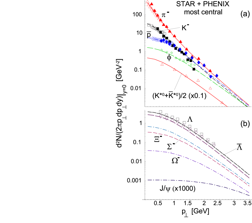
FIG. 1.: (a) The $p_{\perp}$-spectra at midrapidity of pions, kaons, antiprotons, the $\phi$-mesons, and the $K^{*}(892)^{0}$ mesons, and (b) of $\Lambda$, ${\bar{\Lambda}}$, $\Sigma^{-}$, $\Xi^{-}$ , $\Omega^{-}$, and $J/\psi$. The open and filled symbols describe the STAR and PHENIX highest-centrality data, respectively, for $Au+Au$ at $s^{1/2}=130$ GeV A. All theoretical curves and the data are absolutely normalized. The two expansion parameters of the model were fitted to the spectra of pions, kaons, and antiprotons in Ref. [1]. The model curves include full feeding from the weak decays. The data come from Refs. [2,3,31-33]. The STAR data for $\pi^{-},K^{-},\phi$ and $K^{*}$’s are preliminary. The data include full feeding from weak decays.

We recall that the $\phi$ meson deserves a particular attention in relativistic heavy-ion collisions. It serves as a very good “thermometer” of the system, since its interaction with the hadronic environment is negligible. Also, it does not obtain any contribution from the resonance decays, thus its spectrum reflects directly the distribution at freeze-out and the flow.

The upper part of Fig. 1 shows also the averaged spectrum of $K^{*}$’s. In this case the model calculation is compared to the very recently released data [5]. Once again we observe a very good agreement between the model curve and the experimental points. The measured ratios involving the yield of ${K^{*}}(892)^{0}$ [5] also agree well with the output of the thermal model:

$${{\overline{K^{*0}}}\over K^{*0}} = 0.90\hskip 11.38092pt(0.92\pm 0.14)_{\rm expt.}\,,$$ (13)

$${K^{*0}\over h^{-}} = 0.046\hskip 11.38092pt(0.042\pm 0.004\pm 0.01)_{\rm expt.}\,,$$ (14)

$${K^{*0}\over K} = 0.33\hskip 11.38092pt(0.26\pm 0.03\pm 0.07)_{\rm expt.}\,,$$ (15)

$${\phi\over K^{*0}} = 0.42\hskip 11.38092pt(0.49\pm 0.05\pm 0.12)_{\rm expt.}\,.$$ (16)

As already mentioned in the Introduction, the successful description of both the yield and the spectrum of $K^{*}(892)^{0}$ mesons supports the concept of the thermal description of hadron production at RHIC, and brings evidence for small expansion time between chemical and thermal freeze-outs. If the $K^{*}(892)^{0}$ mesons decayed between chemical and thermal freeze-out, the emitted pions and kaons would rescatter and the $K^{*}(892)^{0}$ states could not be reconstructed. In addition, if only a fraction of the $K^{*}(892)^{0}$ yield was reconstructed, it would not agree with the outcome of the thermal analysis which provides the particle yields at the chemical freeze-out. Thus, the expansion time between chemical and thermal freeze-out should be smaller than the $K^{*}(892)^{0}$ lifetime, $\tau=$ 4 fm/$c$ [5].

The lower part of Fig. 1 shows the spectra of strange baryons, and the $J/\psi$ meson. The data for $\Lambda$ and $\overline{\Lambda}$ were taken from Ref. [4]. The $p_{\perp}$-dependence of the spectrum of $\Lambda$ and $\overline{\Lambda}$ is quite satisfactorily reproduced, within 20%, by the model calculation. The other curves in the figure are our predictions.

In Fig. 2 we give the inverse slope parameters for various particles, defined as

$$\lambda_{i}=-\left[\frac{d}{dm_{\perp}}\ln\left(\left.\frac{dN_{i}}{2\pi m_{\perp}dm_{\perp}dy}\right|_{y=0}\right)\right]^{-1}.$$ (17)

This definition reduces to a constant for the exponential spectrum, $\exp(-m_{\perp}/\lambda)$. As can be seen from the figure, the inverse slopes depend strongly on the value of $m_{\perp}$ in the region of interest. The same conclusion has been reached in Ref. [21]. Thus, at least from the viewpoint of our model, it is impossible to describe the spectra in terms of a single slope parameter, as is most commonly practiced in the interpretation of the data. Secondly, the inverse slope increases with the growing mass of the hadron, however this increase is not linear and it is not possible to parameterize it with a simple formula. Recall that the spectra are fed by the decays of resonances, which is an important effect, significantly reducing the inverse slope at lower values of $m_{\perp}$ [12]. The $m_{\perp}$ spectra of pions and kaons are convex , whereas for the remaining particles they are concave, the more the heavier the particle is. All curves in Fig. 2 asymptote to the value

$$\lambda_{\infty}\simeq\frac{T}{\sqrt{1+\rho_{\rm max}^{2}/\tau^{2}}-\rho_{\rm max}/\tau}=363{\rm MeV}.$$ (18)

This formula, specific for our expansion model, is simple to obtain from Eq. (5) with $f_{i}$ given by the exponential form, which is true at large $m_{\perp}$, where the feeding from the resonance decays is absent. As can be seen from Fig. 2, the asymptotics is reached slowly for most of the particles.

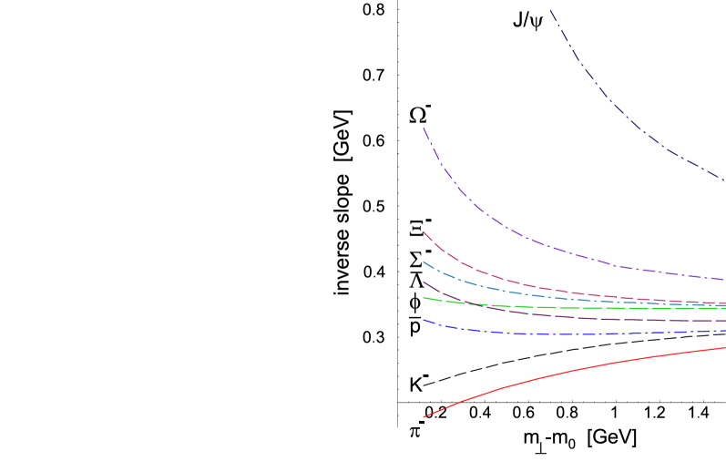
FIG. 2.: The inverse-slope parameters for various particles, calculated as a function of the transverse mass, $m_{\perp}$. The constant $m_{0}$ is the mass of the given particle.

IV Excluded-volume effects

Our fitted values for the geometric parameters $\tau$ and $\rho_{\rm max}$ are low, of the order of the size of the colliding nuclei. This leads to two problems: 1) the values of the HBT radii [46] are too small compared to experiment, and 2) there is little time left for the system to develop large transverse flow. The problems can be helped by the inclusion of the excluded-volume (van der Waals) corrections. Such effects were realized to be important in the earlier studies of the particle multiplicities in relativistic heavy-ion collisions [47, 48, 49], where they led to a significant dilution of system. In the case of the classical (Boltzmann) statistics, which is a very good approximation for our system [50], the excluded volume corrections bring in a factor [48]

$$\frac{e^{-Pv_{i}/T}}{1+\sum_{j}v_{j}e^{-Pv_{j}/T}n_{j}},$$ (19)

into the phase-space integrals, where $P$ is the pressure, $v_{i}=4\frac{4}{3}\pi r_{i}^{3}$ is the excluded volume for the particle of species $i$, and $n_{i}$ is the density of particles of species $i$. The pressure is calculated self-consistently from the equation

$$P=\sum_{i}P^{0}_{i}(T,\mu_{i}-Pv_{i}/T)=\sum_{i}P^{0}_{i}(T,\mu_{i})e^{-Pv_{i}/T},$$ (20)

where $P^{0}_{i}$ is the partial pressure of the ideal gas of hadrons of species $i$. For the simplest case where the excluded volumes for all particles are equal, $r_{i}=r$, the correction manifests itself as a common scale factor, which we denote by $S^{-3}$. The Frye-Cooper formula can then be written in the form [2]

$$\frac{dN_{i}}{d^{2}p_{\perp}dy} = \ \tau^{3}\int_{-\infty}^{+\infty}d\alpha_{\parallel}\int_{0}^{\rho_{\max}/\tau}{\rm sinh}\alpha_{\perp}d\left({\rm sinh}\alpha_{\perp}\right)$$ (22)

$$\times\int_{0}^{2\pi}d\xi\,p\cdot u\,S^{-3}f_{i}\left(p\cdot u\right),$$

where $p\cdot u=m_{\perp}{\rm cosh}\alpha_{\parallel}{\rm cosh}\alpha_{\perp}-p_{\perp}\cos\xi\,{\rm sinh}\alpha_{\perp}$. The emergence of the factor $S^{-3}$ in Eq. (22) may be compensated by rescaling $\rho$ and $\tau$ by the factor $S$. That way the system becomes more dilute and larger in such a way, that the particle multiplicities and the spectra are left intact.

For our values of the thermodynamic parameters, with $\sum_{i}P^{0}_{i}(T,\mu_{i})=80$MeV/fm³, we find $S=1.3$ with $r=0.6$fm, and $S=1.6$ with $r=0.8$fm. Such values of the excluded volumes have been typically used in other calculations. That way, the increase of the size parameters at freeze-out of the order of 30-60% is generated. Therefore, the inclusion of the excluded-volume corrections opens the possibility that the problems 1) and 2) may be alleviated. More detailed analysis will be presented elsewhere.

V Conclusions

The presented model results for the strange hadron production at RHIC support the idea that also these particles are produced thermally. No extra parameters (e.g. strangeness suppression factors) are necessary. This is an important information concerning the particle production mechanism at RHIC. Moreover, the hypothesis of a single freeze-out of Ref. [2] has been additionally verified with the available spectra of $\phi$, $\Lambda$, $\overline{\Lambda}$, and $K^{*}$’s. In short, the thermal model supplied with a suitable parameterization of the freeze-out hypersurface and velocity (i.e. the inclusion of the longitudinal and transverse flow) allows for an efficient and uniform description of the RHIC spectra. A further verification of the model will be provided by the calculation of the HBT correlation radii, as well as the analysis of non-central events, which are currently being examined.

We are grateful to Marek Gaździcki for helpful discussions.

A

Let us consider a sequence of the resonance decays. The initial resonance decouples on the freeze-out hypersurface at the space-time point $x_{N}$, and decays after an average time inversely proportional to the width, $\tau_{N}\approx 1/\Gamma_{N}$. We follow one of the decay products, formed at the point $x_{N-1}$. It decays again after a time $\tau_{N-1}$, and so on. At the end of the cascade a particle with the label 1 is formed, which is directly observed in the experiment. The Lorentz-invariant phase-space density of the measured particles is (we generalize below the formula from Ref. [51] where a single resonance is taken into account)

$$n_{1}\left(x_{1},p_{1}\right)=$$ (A1)

(A2)

$$\int\frac{d^{3}p_{2}}{E_{p_{2}}}B\left(p_{2},p_{1}\right)\int d\tau_{2}\Gamma_{2}e^{-\Gamma_{2}\tau_{2}}$$ (A3)

$$\hskip 28.45274pt\times\int d^{4}x_{2}\delta^{\left(4\right)}\left(x_{2}+\frac{p_{2}\tau_{2}}{m_{2}}-x_{1}\right)...$$ (A4)

(A5)

$$\times\int\frac{d^{3}p_{N}}{E_{p_{N}}}B\left(p_{N},p_{N-1}\right)\int d\tau_{N}\Gamma_{N}e^{-\Gamma_{N}\tau_{N}}$$ (A6)

$$\hskip 28.45274pt\times\int d\Sigma_{\mu}\left(x_{N}\right)\,p_{N}^{\mu}\,\,\delta^{\left(4\right)}\left(x_{N}+\frac{p_{N}\,\tau_{N}}{m_{N}}-x_{N-1}\right)$$ (A7)

$$\hskip 42.67912pt\times\,f_{N}\left[p_{N}\cdot u\left(x_{N}\right)\right],$$ (A8)

(A9)

where $B(q,k)$ is the probability for a resonance with momentum $k$ to produce a particle with momentum $q$, namely

$$B(q,k)={b\over 4\pi p^{*}}\delta\left({k\cdot q\over m_{R}}-E^{*}\right).$$ (A10)

Here $b$ is the branching ratio for the particular decay channel, and $p^{*}$ ($E^{*}$) is the momentum (energy) of the emitted particle in the resonance’s rest frame. Integration over all space-time positions gives the momentum distribution

$$E_{p_{1}}{dN_{1}\over d^{3}p_{1}}=\int d^{4}x_{1}\,n_{1}\left(x_{1},p_{1}\right)$$ (A11)

$$= \int\frac{d^{3}p_{2}}{E_{p_{2}}}B\left(p_{2},p_{1}\right)...\int\frac{d^{3}p_{N}}{E_{p_{N}}}B\left(p_{N},p_{N-1}\right)$$ (A13)

$$\times\int d\Sigma_{\mu}\left(x_{N}\right)\,p_{N}^{\mu}\,\,f_{N}\left[p_{N}\cdot u\left(x_{N}\right)\right],$$

which should be used in a general case. Note that the dependence on the widths $\Gamma_{k}$ has disappeared, reflecting the fact that it is not relevant when or where the resonances decay.

A simplification follows if the element of the freeze-out hypersurface is proportional to the four-velocity (this is exactly the case considered in our model defined by Eqs. (1) and (2)),

$$d\Sigma_{\mu}(x_{N})=d\Sigma(x_{N})\,u_{\mu}(x_{N}).$$ (A15)

Then

$$E_{p_{1}}{dN_{1}\over d^{3}p_{1}}=\int d\Sigma\left(x_{N}\right)\int\frac{d^{3}p_{2}}{E_{p_{2}}}B\left(p_{2},p_{1}\right)...$$ (A17)

$$\times\int\frac{d^{3}p_{N}}{E_{p_{N}}}B\left(p_{N},p_{N-1}\right)p_{N}\,\cdot u\left(x_{N}\right)\,f_{N}\left[p_{N}\cdot u\left(x_{N}\right)\right]$$

$$= \int d\Sigma\left(x_{N}\right)p_{1}\,\cdot u\left(x_{N}\right)\,f_{1}\left[p_{1}\cdot u\left(x_{N}\right)\right],$$ (A18)

where we have introduced the transformation

$$p_{k-1}\,\cdot u\left(x_{N}\right)\,f_{k-1}\left[p_{k-1}\cdot u\left(x_{N}\right)\right]$$ (A19)

$$=\int\frac{d^{3}p_{k}}{E_{p_{k}}}B\left(p_{k},p_{k-1}\right)p_{k}\,\cdot u\left(x_{N}\right)\,f_{k}\left[p_{k}\cdot u\left(x_{N}\right)\right],$$ (A20)

(A21)

which can be used (step by step along the cascade) to calculate the distribution of the measured particles. In the fluid local-rest-frame, most convenient in the numerical calculation, we have $u^{\mu}(x_{N})=(1,0,0,0)$, and the transformation (A21) reduces to the form discussed in [12]. A technical simplification relies in the fact that in Eq. (A18) the space-time integration over the hypersurface is performed at the end, consequently the momentum integration in Eq. (A21) preserves the full spherical symmetry. That way, the momentum integrals are one-dimensional and the numerical procedure is very fast. On the other hand, in the general case of Eq. (LABEL:npip1) the integration over the hyper-surface has to be done first, reducing the symmetry of the following momenta integrals. The symmetry is cylindrical, thus the momentum integrals are two-dimensional. Moreover the integrands have an integrable singularity, which make the numerical procedure more involved [51, 52].

REFERENCES

- [1] Supported in part by the Polish State Committee for Scientific Research, grant 2 P03B 09419.
- [2] W. Broniowski and W. Florkowski, Phys. Rev. Lett. 87, 272302 (2001).
- [3] E. T. Yamamoto, hep-ph/0112017.
- [4] C. Adler et al., STAR Collaboration, nucl-ex/0203016.
- [5] P. Fachini, STAR Collaboration, nucl-ex/0203019.
- [6] J. Rafelski and B. Müller, Phys. Rev. Lett. 48, 1066 (1982).
- [7] P. Koch, B. Müller, and J. Rafelski, Phys. Rep. 142, 167 (1986).
- [8] J. Rafelski and J. Letessier, hep-ph/0112027.
- [9] C. P. Singh, Phys. Rep. 236, 147 (1993).
- [10] P. Braun-Munzinger, I. Heppe, and J. Stachel, Phys. Lett. B 465 , 15 (1999).
- [11] P. Braun-Munzinger, D. Magestro, K. Redlich, and J. Stachel, Phys. Lett. B 518, 41 (2001).
- [12] W. Florkowski, W. Broniowski, and M. Michalec, Acta Phys. Pol. B 33, 761 (2002).
- [13] U. Heinz, Nucl. Phys. A 661, 140c (1999).
- [14] J. Rafelski and J. Letessier, Phys. Rev. Lett. 85, 4695 (2000).
- [15] Particle Data Group, Eur. Phys. J. C 15, 1 (2000).
- [16] R. Hagedorn, CERN preprint No. CERN-TH.7190/94 (1994), and references therein.
- [17] J. D. Bjorken, Phys. Rev. D 27, 140 (1983).
- [18] G. Baym, B. Friman, J.-P. Blaizot, M. Soyeur, and W. Czyż, Nucl. Phys. A 407, 541 (1983).
- [19] P. Milyutin and N. N. Nikolaev, Heavy Ion Phys 8, 333 (1998); V. Fortov, P. Milyutin, and N. N. Nikolaev, JETP Lett. 68, 191 (1998).
- [20] P. J. Siemens and J. Rasmussen, Phys. Rev. Lett. 42, 880 (1979); P. J. Siemens and J. I. Kapusta, Phys. Rev. Lett. 43, 1486 (1979).
- [21] E. Schnedermann, J. Sollfrank, and U. Heinz, Phys. Rev. C 48, 2462 (1993).
- [22] T. Csörgő and B. Lörstad, Phys. Rev. C 54, 1390 (1996).
- [23] D. H. Rischke and M. Gyulassy, Nucl. Phys. A 697, 701 (1996); Nucl. Phys. A 608, 479 (1996).
- [24] R. Scheibl and U. Heinz, Phys. Rev. C 59, 1585 (1999).
- [25] K. A. Bugaev, Nucl. Phys. A 606, 559 (1996).
- [26] L. P. Csernai, Zs. I. Lázár, and D. Molnár, Heavy Ion Phys. 5, 467 (1997).
- [27] J. J. Neymann, B. Lavrenchuk, and G. Fai, Heavy Ion Phys. 5, 27 (1997).
- [28] V. K. Magas et al., Nucl. Phys. A 661, 596c (1999).
- [29] F. Cooper, G. Frye, and E. Schonberg, Phys. Rev. D 11, 192 (1975).
- [30] T. S. Biró, Phys. Lett. B 474, 21 (2000); Phys. Lett. B 487, 133 (2000).
- [31] K. S. Lee, U. Heinz, and E. Schnedermann, Zeit. f. Phys. C 48, 525 (1990).
- [32] J. Velkovska, PHENIX Collaboration, Nucl. Phys. A 698, 507 (2002).
- [33] J. Harris, STAR Collaboration, talk presented at QM2001.
- [34] C. Adler et al., STAR Collaboration, Phys. Rev. Lett. 87, 262302 (2001).
- [35] F. Cooper and G. Frye, Phys. Rev. D 10, 186 (1974).
- [36] W. Broniowski and W. Florkowski, Phys. Lett. B 490, 223 (2000).
- [37] W. Broniowski, in Proc. of Few-Quark Problems, Bled, Slovenia, July 8-15, 2000, eds. B. Golli, M. Rosina, and S. Širca, p. 14, hep-ph/0008122.
- [38] M. Gaździcki and M. I. Gorenstein, Phys. Rev. Lett. 83, 4009 (1999).
- [39] K. A. Bugaev, M. Gaździcki, and M. I. Gorenstein, Phys. Lett. B 523, 255 (2001).
- [40] L. Grandchamp and R. Rapp, Phys. Lett. B 523, 60 (2001).
- [41] P. Braun-Munzinger and J. Stachel, Nucl. Phys. A 690, 119 (2001); Phys. Lett. B 490, 196 (2000).
- [42] P. Huovinen, P. F. Kolb, U. Heinz, P. V. Ruuskanen, and S. A. Voloshin, Phys. Lett. B 503, 58 (2001).
- [43] D. Teaney, J. Lauret, and E. V. Shuryak, Phys. Rev. Lett. 86, 4783 (2001); Nucl. Phys. A 698, 479 (2002).
- [44] T. Hirano, Phys. Rev. C 65, 011901 (2002); T. Hirano, K. Morita, S. Muroya, and C. Nonaka, nucl-th/0110009.
- [45] A. Ster and T. Csörgő, hep-ph/0112064.
- [46] C. Adler et al., STAR Collaboration, Phys. Rev. Lett. 87, 082301 (2001).
- [47] P. Braun-Munzinger, J. Stachel, J. P. Wessels, and N. Xu, Phys. Lett. B 344, 43 (1995); Phys. Lett. B 365, 1 (1996).
- [48] G. D. Yen, M. I. Gorenstein, W. Greiner, and S. N. Yang, Phys. Rev. C 56, 2210 (1997).
- [49] G. D. Yen and M. I. Gorenstein, Phys. Rev. C 59, 2788 (1999).
- [50] M. Michalec, PhD Thesis, nucl-th/0112044.
- [51] J. Bolz, U. Ornik, M. Plümer, B.R. Schlei, and R.M. Weiner, Phys. Rev. D 47, 3860 (1993).
- [52] J. Sollfrank, P. Koch, and U. Heinz, Phys. Lett. B 252, 256 (1990).