Reconstruction of Hadronization Stage in Pb+Pb Collisions at 158A GeV/c

Abstract

Recent data on hadron multiplicities in central Pb+Pb collisions at 158A GeV/c at mid-rapidity are analyzed within the concept of chemical freeze-out. A non-uniformity of the baryon chemical potential along the beam axis is taken into account. An approximate analytical solution of the hydrodynamic equations for a chemically frozen Boltzmann-like gas is found. The Cauchy conditions for hydrodynamic evolution of the hadron resonance gas are fixed at the thermal freeze-out hypersurface from analysis of one-particle momentum spectra and HBT correlations. The proper time of chemical freeze-out and physical conditions at the hadronization stage, such as energy density and averaged transverse velocity, are found.

I Introduction

Systems which are created in ultra-relativistic A+A collisions at SPS and RHIC are initially very dense and display collective behavior. The quasi-macroscopic nature of those systems allows to study new states of matter at the phase boundary between a hadron gas (HG) and the quark-gluon plasma (QGP). Among the different methods to study it, an important role belongs to precise measurement of hadronic observables. One- and multi-particle hadron spectra, however, do not carry direct information about the phase transition since one should expect strong interactions in the hadron resonance gas after hadronization. Usually, different theoretical approaches are used to diagnose the matter properties at the transition point. A rather fruitful concept is that of chemical freeze-out. It implies, first, that the initial hadronic state is in chemical equilibrium [1, 2, 3]. Second, the chemical concentrations of HG do not change during the evolution. The latter assumption is justified by the observation that the rate of expansion in HG is larger than the rate of inelastic reactions and less than that of elastic collisions [4].

It gives the possibility to use the approach of local thermal equilibrium and hydrodynamic expansion of HG at approximately frozen chemical composition. The initial conditions for the hadronic stage of the collective expansion are determined by matter evolution in the pre-hadronic phase and also by particle interactions and hadronization conditions.

If chemical freeze-out takes place, it is defined by a temperature and chemical potentials conjugated to conserved quantum numbers. To extract those thermodynamic parameters from total particle number ratios one has to assume uniform temperature, baryon and strangeness chemical potentials as well as a unique hadronization hypersurface $\sigma^{ch}(x)$ for all particles. The result is a common effective volume for all hadron species, that completely absorbs effects of flow and a form of the hypersurface and approximately cancels in a description of particle ratios [5, 6].

In detail, the situation may be somewhat more complicated. While baryon stopping seems to be fairly complete at AGS energies [7] (see also Ref.[8] where possible deviations from the full stopping are analyzed quantitatively), there are clear indications for an onset of transparency at top SPS energy from the observed fairly flat rapidity distribution of pions in Pb+Pb central collisions [9, 10] and, in particular, from the difference in rapidity distributions between protons and antiprotons, which cannot be explained by longitudinal flow developing after full stopping. As a consequence, one could expect particle number ratios taken in mid-rapidity, especially involving nucleons, to differ somewhat from those integrated over $4\pi$. On the other hand, a consistent hydrodynamic analysis then must be based on an analysis of data in a narrow mid-rapidity region, which is done in this paper. We also note that, in a boost-invariant scenario as observed at RHIC, chemical freeze-out conditions are the same for any individual rapidity slices taken within a wide enough rapidity interval.

The object of this paper is to reconstruct the hadronization stage within the hydrodynamic approach. We assume that hadronic matter at that stage has locally a maximal entropy. Effects of hadron-hadron interaction (excluded volumes [11], mean field [12]) as well as specific conditions of hadronization (e.g., possible conservation of number of quarks during the hadronization [13] ) are rather complicated and model dependent. So it is naturally to use minimal number of parameters and take all that into account in the simplest way, i.e., as a unique factor changing the particle numbers. In other words, we describe the system at the stage of hadronization as a mixture of ideal gases with additional common chemical potential $\mu_{ch}$. Afterwards the system expands hydrodynamically with frozen chemical composition, cools down and finally decays at some thermal freeze-out hypersurface $\sigma^{th}(x)$ which could be different for different particle species [14, 15, 16]. Then long-lived particles stream freely into detectors, resonances decay and also contribute to spectra of observed particles. We reconstruct a state of the system at the earlier hadronization stage, find energy and particle number densities and also estimate roughly the effects of interaction at the hadronization stage using an approach described in the following.

From the analysis of slopes of transverse momentum spectra and of interferometry radii for different particle species one can restore the space-time extensions, collective flow parameters and temperature at the thermal freeze-out stage, when the thermal system decouples and particle momentum distributions change no longer. The method of joint analysis of the spectra and correlations was used in Refs. [5, 17, 18, 19] to reconstruct the thermal freeze-out stage. Note that, to evaluate the detailed behavior of the (pion) spectrum in the whole transverse momentum region, one needs in detail knowledge of the unobserved resonance yields. They can be estimated from the temperature and baryochemical potential at chemical freeze-out. An attempt to determine the resonance yields in that way was undertaken in Ref. [18]. There however, a trajectory assuming isentropic expansion in full chemical equilibrium was employed following Ref. [14], in contradistinction to the assumption of chemical freeze-out. In this paper we make a new analysis of the thermal freeze-out stage within the hydrodynamic approach for lead-lead collisions based on recent experimental data on one particle spectra and HBT correlations for different hadron species. We estimate the basic parameters at thermal freeze-out from an analysis of the slopes of particle spectra and of the correlation functions at regions of high enough transverse momentum to minimize the influence of resonance decays. We use also the previous results from Refs.[18, 19] to determine the influence of uncertainties in reconstruction of the thermal freeze-out stage on the reconstruction of the hadronic gas parameters at chemical freeze-out.

Recent evidence [1, 2, 3, 20] support strongly the early interpretation [21] that chemical freeze-out at SPS and higher energies takes place at or near to the phase boundary (see also the discussion in [22]). We employ a similar approach here with emphasis on the analysis of particle ratios near mid-rapidity. To complete the reconstruction of the hadronization stage and find its space-time extension, we solve the hydrodynamic equations with the Cauchy conditions that are found at thermal freeze-out, and consider the solution backwards in time until the chemical freeze-out temperature is reached. The method leads to unique results due to the scale invariance of the hydrodynamic equations for a mixture of ideal Boltzmann gases with reference to scale-transformations of pressure and densities of energy and particles at a fixed temperature. For such a system the variation of initial densities by a unique factor results in the same scale transformation of the solutions. Therefore, the temperature as function of time does not depend on the common chemical potential, which defines absolute values of densities: the temperature depends only on concentrations of different particles species. The latter do not change during the hydrodynamic evolution and are determined by the baryonic and strangeness chemical potentials and temperature just after hadronization. Finally, from reconstructed space-time extension of the chemical freeze-out and a particle numbers in mid-rapidity we determine the densities at hadronization and the common chemical potential.

An alternative way to determine hadron gas parameters is used in Ref. [14]. There, a hydrodynamic approach is followed from the initial condition of an equilibrated QGP through the phase transition and hadronization. Subsequent to hadronization the system is assumed, in fact, to evolve as a mixture of mutually non-interacting gases with fixed chemical composition. In the present approach we, instead, solve the hydrodynamic equations for a complete system under the explicit condition of particle numbers conservation. The distinctive feature of our method is the analysis backwards in time.

One more important point which we would like to comment here concerns the question of applicability of the hydrodynamic approach to post hadronization stage in A+A collisions. In recent papers [16, 23] it is stated that the hydrodynamic approach is unable to describe the stage of hadron phase expansion in heavy ion collisions. Note, however, that the criticism of Refs. [16, 23] as to the hydrodynamics is based on calculations of chemically equilibrium evolution of the mixture of hadron gases. This evolution differs essentially from the evolution of chemically frozen gas [24, 25]. In very recent work [25] the first detailed comparisons of RQMD calculations with chemically frozen hydrodynamics were done. There it was demonstrated that if chemical freeze-out is incorporated into the hydrodynamics, then the final spectra and fireball lifetimes are insensitive to the temperature at which the switch from hydrodynamics to cascade is made. It implies that the transformation of heat energy into collective flow for a chemically frozen hydrodynamic evolution results in spectra which correspond approximately to the microscopic cascade calculations. Moreover, the initial conditions of hydro-expansion in Refs. [16, 23] correspond to chemically equilibrium mixture of Boltzmann hadronic gases and does not include possible specific effects of hadronization process, excluded volumes and collective interaction. The estimation of these effects, which may reducing the particle number, is one of the important aims of this paper. Therefore, the criticism in Refs [16, 23] as to applicability of hydrodynamics is based on the hydrodynamic models which differ essentially from what is used in our paper. The opposite to Refs. [16, 23] conclusion as to applicability of hydrodynamics to the post hadronization stage in A+A collisions, was argued recently in Refs. [26]. There it was shown, in particular, that the hydrodynamics describes good the single particle spectra and elliptic flows also in RHIC experiments.

Nevertheless, the cascade models [15, 16, 23] of post hadronization stage are considered now as favorable alternative to the hydrodynamic approach. The picture of evolution and particle emission are rather different in hydrodynamic approach and cascade models (RQMD, UrQMD, etc…). While in standard hydrodynamic picture the particle spectra are evaluated usually according to the Cooper-Frye prescription [27] (using the freeze-out hypersurfaces), the cascade calculations does not demonstrate the sharp region of particle emission [15]. It does not mean, however, that hydrodynamic description is incorrect: the absence of principal contradictions between the both methods of spectra calculations was demonstrated quite recently in Ref. [28] based on exact solution of Boltzmann equation. The method of escape probabilities, proposed there, gives possibility to make bridge between hydrodynamic and transport models for rarefied systems. As to rather dense systems, similar to those that form just after hadronization, where the time of collision is similar to the time between collisions and collective effects, such as multiparticle collisions and modification of hadron properties, may take place, the oversimplified version of transport approach, like UrQMD, cannot be applied correctly while hydrodynamic approach is more suitable. Note also that at CERN SPS and RHIC energies the cascade models fail actually to describe the interferometry radii of the system (see, e.g., [29, 23]).

In Sec. II we discuss the possibility to extract the thermodynamic parameters at chemical freeze-out from the particle number ratios when those parameters are non-uniformly distributed in rapidity. In Sec. III we consider the particle number ratios in a hydrodynamic approach to A+A collisions. The optimization procedure is applied to fit recent experimental data for Pb+Pb (CERN, SPS) collisions and find the temperature, baryonic and strangeness chemical potentials at chemical freeze-out. In Sec. IV we analyze the property of hydrodynamic expansion in a central slice of space-time rapidity for a chemically frozen mixture of ideal Boltzmann gases. Approximate hydrodynamic solutions for non-relativistic transverse flows are found. In Sec.V the Cauchy conditions at thermal freeze-out, such as proper time, transverse Gaussian radius parameter, temperature and transverse velocities are defined from the analysis of spectra and HBT correlations. In Sec.VI the corresponding “ inverse in time” hydrodynamic solution is analyzed and the space-time characteristics of the matter at the hadronization stage are reconstructed. The later are applied to restore the energy and particle number densities at that stage. The conclusions and a discussion of the results are presented in Sec.VII.

II The particle numbers at mid-rapidity for expanding HG

We assume that just after hadronization, the system can be described at some hypersurface $\sigma^{ch}(x)$ as a locally and chemically equilibrated expanding hadron resonance gas. The effects of interaction and possible peculiarities of the hadronizaton process are taken into account by a common factor changing particle numbers in the ideal gas; the factor is associated with an additional common chemical potential $\mu_{ch}$. In concrete evaluations, as was performed by many authors, instead of considering a finite chemical and thermal freeze-out hypersurfaces $\sigma(x)$ in Minkovsky space, we use the common profile factor $\rho(x)$ at proper time $\tau(r)\approx const$ to guarantee the finiteness of the system (see the discussion on the validity of such an approximation in [17]). Then the total multiplicity of a particle species $i$ at chemical freeze-out is calculated by

$$N_{i}=\int\frac{d^{3}p}{p^{0}}d\sigma_{\mu}^{ch}(x)p^{\mu}f\left(\frac{p_{\mu}u^{\mu}(x)}{T_{ch}(x)},\frac{\mu_{i,ch}(x)}{T_{ch}(x)}\right)\rho(x),$$ (1)

where $f(p_{\mu}u^{\mu}(x)/T_{ch}(x),\mu_{i,ch}(x)/T_{ch}(x))$ is the Bose-Einstein or Fermi-Dirac distribution function in our approach , and $\mu_{i,ch}=B_{i}\mu_{B}+S_{i}\mu_{S}+\mu_{ch}$. The additional chemical potential $\mu_{ch}$ is unique for all particles species. The effect of isotopic chemical potential has been investigated in [3] and found to be small. It is neglected in this paper. Taking into account the invariance of the distribution function under Lorentz transformation, one can carry out integrations over momentum variables and finally get

$$N_{i}=\int d\sigma_{\mu}^{ch}(x)u^{\mu}(x)n_{i}^{ch}(x),\quad n_{i}^{ch}(x)=\overline{n}_{i}^{ch}(x)\rho(x)$$ (2)

where in Boltzmann approximation for the distribution function the thermodynamic densities $\overline{n}_{i}^{ch}(x)$ have the form

$$\overline{n}_{i}^{ch}(x)=\frac{(2J_{i}+1)}{2\pi^{2}}T_{ch}(x)m_{i}^{2}\exp(\mu_{i,ch}(x)/T_{ch}(x))K_{2}(m_{i}/T_{ch}(x)),$$ (3)

and $K_{n}(u)=\frac{1}{2}\int_{-\infty}^{+\infty}dz\exp[-u\cosh z+nz]$ , with $\mathop{\rm Re}u>0,$ is the modified Bessel function of order $n$ ($n=0,1,...$). One can rewrite (2) in the form

$$N_{i}=\langle\overline{n}_{i}^{ch}\rangle V^{ch}$$ (4)

where the volume $V^{ch}$ of system is expressed through the integral of the hydrodynamic $4$ -velocity $u^{\mu}(x)$ and the profile factor $\rho(x)$ over the hypersurface $\sigma^{ch}$:

$$V^{ch}=\int d\sigma_{\mu}^{ch}(x)u^{\mu}(x)\rho(x).$$ (5)

We further define the density averaged over the chemical freeze-out hypersurface by

$$\langle\overline{n}_{i}^{ch}\rangle=\frac{\int d\sigma_{\mu}^{ch}u^{\mu}(x)\overline{n}_{i}^{ch}(x)\rho(x)}{\int d\sigma_{\mu}^{ch}u^{\mu}(x)\rho(x)}.$$ (6)

If temperature and chemical potentials are uniform over the chemical freeze-out hypersurface, then $\langle\overline{n}_{i}^{ch}\rangle=\overline{n}_{i}^{ch}(T_{ch},\mu_{i,ch})$ and the standard analysis of particle number ratios in $4\pi$ geometry can be performed to find the temperature and chemical potentials. However, if $T$ and $\mu$ are not uniformly distributed over the hydrodynamic tube at the hypersurface $\sigma^{ch}$, then the similar analysis implying the substitution $\langle\overline{n}_{i}\rangle\rightarrow\overline{n}_{i}^{ch}(\langle T_{ch}\rangle,\langle\mu_{i,ch}\rangle)$ with some average temperature and chemical potentials, could result in significant deviations for the values one is interested in [30]. To reduce the corresponding uncertainties, the analysis of particle ratios in a narrow rapidity interval near mid-rapidity should be used as we will discuss below.

To analyze non-uniformly distributed systems, let us start from the well known observation [31] that, at the latest stage of a hydrodynamic evolution, the longitudinal velocity distribution corresponds to the asymptotic quasi-inertial regime, $v_{L}=z/t$. This property, which is the ansatz in the Bjorken model [32] for each moment of time, is realized at the freeze-out stage even in the Landau model of complete stopping [31]. Consequently, we assume in the following the boost-invariance for longitudinal hydrodynamic velocities at the last (hadronic) stage of the evolution, $v_{L}=z/t$. This then allows us to parameterize $t$ and $z$ at $\sigma$ by the form: $t=\tau(r,\eta)\cosh(\eta)$, $z=\tau(r,\eta)\sinh(\eta)$, where $r$ is absolute value of the transverse coordinate ${\bf{r}}$ and $\eta$ is the longitudinal fluid rapidity, $\eta=\tanh^{-1}v_{L}$. The parameter $\tau(r,\eta)$ generalizes the Bjorken proper time parameter $\tau$. Taking into account also a transverse velocity component ($v(r,\tau)$ in the longitudinally co-moving system, LCMS), we obtain for the 4-velocity

$$u^{\mu}(r,\eta)=\gamma\left(\cosh\eta,v\cos\phi,v\sin\phi,\sinh\eta\right),$$ (7)

where $\gamma=(1-v^{2})^{-1/2}$. The element of the hypersurface $\sigma(x)$ takes the form

$$d\sigma_{\mu}=\tau(r,\eta)d\eta dr_{x}dr_{y}\left(\frac{1}{\tau}\frac{d\tau}{d\eta}\sinh\eta+\cosh\eta,-\frac{d\tau}{d{r}_{x}},-\frac{d\tau}{d{r}_{y}},-\frac{1}{\tau}\frac{d\tau}{d\eta}\cosh\eta-\sinh\eta\right).$$ (8)

Let us, first, introduce for an expanding HG the effective volume $V_{eff}$ attributed to one unit of rapidity. To determine $V_{eff}$ one can write the particle number distribution differential in fluid rapidity $\eta$ for particle of species $"i"$ at chemical freeze-out:

$$\frac{dN_{i}}{d\eta}=\int\frac{d^{3}p}{p^{0}}\frac{d\sigma_{\mu}^{ch}}{d\eta}p^{\mu}f\left(\frac{p_{\mu}u^{\mu}(r,\eta)}{T_{ch}(\eta)},\frac{\mu_{i,ch}(\eta)}{T_{ch}(\eta)}\right)\rho(r,\eta).$$ (9)

Here we assume that the chemical potentials as well as the temperature are constants in transverse direction across the freeze-out hypersurface. Taking into account the invariance of the distribution function under Lorentz transformation, one can carry out integrations over momentum variables and finally gets

$$\frac{dN_{i}}{d\eta}=V_{eff}^{ch}(\eta)\overline{n}_{i}^{ch}(\eta)$$ (10)

and

$$V_{eff}^{ch}(\eta)=\int\frac{d\sigma_{\mu}^{ch}}{d\eta}u^{\mu}(r,\eta)\rho(r,\eta).$$ (11)

The particle number distribution over momentum rapidity $y$ is

$$\frac{dN_{i}}{dy}=\int\frac{d^{3}p}{p^{0}dy}d\sigma_{\mu}^{ch}p^{\mu}f\left(\frac{p_{\mu}u^{\mu}(r,\eta)}{T_{ch}(\eta)},\frac{\mu_{i,ch}(\eta)}{T_{ch}(\eta)}\right)\rho(r,\eta).$$ (12)

One can rewrite Eq. (12) in the form

$$\frac{dN_{i}}{dy}=\frac{dN_{i}}{d\eta}\mid_{\eta=y}(1+\delta_{i}(y))=V_{eff}^{ch}(y)(1+\delta_{i}(y))\overline{n}_{i}^{ch}(y)$$ (13)

where

$$\delta_{i}(y)=\frac{\frac{dN_{i}}{dy}-\frac{dN_{i}}{d\eta}\mid_{\eta=y}}{\frac{dN_{i}}{d\eta}\mid_{\eta=y}}$$ (14)

From Eq. (13), one can conclude that, for a nonuniform distribution of thermodynamic parameters along the beam axis, the analysis of particle number ratios at mid-rapidity, $y\approx 0$ can be based on ratios $\overline{n}_{i}/\overline{n}_{j}$ if correction factors $\delta_{i}(0)$ are small. One can include corresponding corrections in the non-unique “effective volume” $V_{eff,i}^{ch}=V_{eff}^{ch}(1+\delta_{i})$ which is different for different particle species.

Let us estimate the correction factors. The saddle-point approximation to the integrals over fluid rapidity $\eta$ in (12) can be applied when the parameter $m_{i}/T(\eta)\gg 1$ at the saddle point $\eta\approx y$. Then, at mid-rapidity, the area around $\eta=y=0$ gives the main contribution to the integral over $\eta$ in (12) and one can expand the slowly varying functions into a Tailor series around the saddle-point $\eta=0$. For the sake of simplicity, we neglect a variation of $T(\eta)$ in space rapidity $\eta$ in comparison with the variation of $\mu_{i}^{ch}(\eta)$, assuming that all non-uniformity originated from incomplete baryonic stopping. This implies an increase of the baryonic chemical potential with the absolute value of rapidity. Assuming that the transverse expansion is non-relativistic, with a freeze-out that occurs at approximately equal proper time $\tau$, and that the profile $\rho(x)$ can be factorized, $\rho(x)=\rho_{T}(r)\rho_{L}(\eta)$, we estimate the correction factor at mid-rapidity:

$$\delta_{i}\approx\frac{1}{2}\frac{(\rho_{L}\exp(\mu_{i,ch}/T_{ch})\tau_{ch})^{\prime\prime}\mid_{\eta=0}}{\rho_{L}(0)\exp(\mu_{i,ch}/T_{ch})\tau_{ch}}\frac{T_{ch}}{m_{i}}$$ (15)

All thermodynamic parameters here are taken at mid-rapidity. One can see that the factor $\delta_{i}$ is rather small for baryons, because the ratio $T_{ch}/m_{i}$ is small, as well as it is small for pions, because their baryonic number are equal to zero. Therefore, as follows from Eq.(13) for $\delta_{i}\ll 1$ the analysis of particle number ratios at a narrow mid-rapidity interval can be based on ratios $\overline{n}_{i}^{ch}/\overline{n}_{j}^{ch}$ [5]. These values are the same as for Boltzmann gas in a static volume [5, 6].

It is worth to note that the second derivative in formula (15) is positive for incomplete baryonic stopping and, so, $\delta_{i}>0$. As we will discuss later, the consequences of it are non-trivial and rather important for pion production via decay of baryonic resonances after the thermal freeze-out occurs.

III The analysis of particle number ratios

In ultrarelativistic A+A collisions a hadron resonance gas is assumed to appear due to the hadronization process. Subsequent, it expands and reaches the final stage of the evolution - the thermal freeze-out. According to the hypotheses of chemical freeze-out, the total number of each particle species is preserved during the evolution. After the hydrodynamic tube decays and produces final particles, one has to take into account also particles that come from resonance decays. In our calculations the resonance mass spectrum extends over all mesons and baryons with masses below $2$ GeV. Decay cascades are also included in the analysis. The value of the strangeness chemical potential $\mu_{S}$ is fixed by baryonic chemical potential and temperature from the condition of local strangeness conservation. We optimize the particle number ratios at mid-rapidity, using the corresponding values for Pb + Pb collisions at 158A GeV/c from WA97 (Table 1) and NA49 (Table 2) experiments, excluding from optimization procedure pions as the lightest particles, the later circumstance can result in serious corrections, besides of Bose-Einstein enhancement effect in the distribution function, which we will discuss below. Then we describe the data in the model of a chemically equilibrated ideal hadron gas (HG). The feeding in our calculations is tuned according to the experimental conditions as described below.

In the geometry of the WA97 experiment the feed-down from weak cascade decays is expected to be of minor importance [34], and so the $\Lambda$ ($\overline{\Lambda}$) have not been corrected for feed-down from $\Xi$ weak decays, and $\Xi$ have not been corrected for feed-down from $\Omega$. But feeding of $\Lambda$ ($\overline{\Lambda}$) from electromagnetic decays of $\Sigma^{0}$ ($\overline{\Sigma}^{0}$) is included. We did not include (according to the NA49 experimental procedure [10]) feeding of $p$ and $\overline{p}$ from $\overline{\Lambda},$ $\Lambda$ and from $\Sigma^{+},\overline{\Sigma}^{+}$. In the NA49 experiment $\Lambda$ and $\overline{\Lambda}$ yields include the contributions of $\Sigma^{0}$ and $\overline{\Sigma}^{0}$ as well as feed-down from weak $\Xi$ decays [10]. The feeding of $\pi^{-}$ from kaons and from $\Lambda$ is not included [9]. We included feeding from $\phi$ decay into kaons (NA49 and WA97) and pions (NA49). For technical reasons in the model calculations we used the following substitution: $K_{s}^{0}/\pi^{-}\rightarrow(K^{-}+K^{+})/2\pi^{-}$, a good approximation for Pb+Pb collisions [35]. The results for the best fit are shown in Tables 1 and 2 for Boltzmann statistic (BS) and quantum statistic (QS) calculations. The obtained temperatures $T_{ch}\approx 164$ MeV and baryochemical potential $\mu_{B}\approx 224$ MeV differ slightly from the corresponding values of Ref. [3], $T_{ch}\approx 168$ MeV, $\mu_{B}\approx 266$ MeV, that were gotten from analysis of particle number ratios in different limited rapidity intervals as well as in full $4\pi$-geometry.

TABLE 1. Experimental particle number ratios (WA97) in Pb+Pb SPS collisions , compared to model calculation for Boltzmann statistic (BS) and quantum statistic (QS)

$T_{ch}$		$163.37$ MeV	$163.91$ MeV
$\mu_{B}$		$223.6$ MeV	$224.0$ MeV
$\mu_{S}$		$55.2$ MeV	$55.1$ MeV
Ratios	Data	BS	QS
$\overline{\Lambda}/\Lambda$	$0.133\pm 0.007$ [34]	$0.133$	$0.133$
$\Xi^{+}/\Xi^{-}$	$0.249\pm 0.019$ [34]	$0.250$	$0.249$
$\Xi^{-}/\Lambda$	$0.100\pm 0.004$ [34]	$0.098$	$0.099$
$\Xi^{+}/\overline{\Lambda}$	$0.188\pm 0.016$ [34]	$0.186$	$0.186$
$\Omega^{-}/\Xi^{-}$	$0.182\pm 0.022$ [34]	$0.139$	$0.140$
$\Omega^{+}/\Xi^{+}$	$0.281\pm 0.053$ [34]	$0.274$	$0.274$
$\Omega^{+}/\Omega^{-}$	$0.383\pm 0.081$ [34]	$0.492$	$0.489$
$\Lambda/K_{s}^{0}$	$0.6706$ [36]	$0.6212$	$0.6226$

TABLE 2. Experimental particle number ratios (NA49) in Pb+Pb SPS collisions , compared to model calculation for Boltzmann statistic (BS) and quantum statistic (QS).

$T_{ch}$		$163.37$ MeV	$163.91$ MeV
$\mu_{B}$		$223.6$ MeV	$224.0$ MeV
$\mu_{S}$		$55.2$ MeV	$55.1$ MeV
Ratios	Data	BS	QS
$(p-\overline{p})/\pi^{-}$	$0.184$ [9]	$0.245$	$0.239$
$(p-\overline{p})/K^{-}$	$1.776$ [9, 35]	$1.847$	$1.843$
$(p-\overline{p})/K^{+}$	$1.028$ [9, 35]	$1.090$	$1.086$
$K^{+}/K^{-}$	$1.727$ [35]	$1.695$	$1.697$
$\overline{p}/p$	$0.115$ [9]	$0.066$	$0.067$
$\phi/(p-\overline{p})$	$0.0802$ [9, 35, 37]	$0.0937$	$0.0935$

The deviation between calculated particle ratios and experimental data are within the error of the data of WA97, excepts for the ratios which contain $\Omega$. As to the $\overline{p}/p$ ratio of NA49, one has take into account that the corresponding data $\overline{p}/p\approx 0.11$ are rather preliminary and differ much from published NA44 data where the value is twice less [38]. It is interesting to note, that in rapidity interval $2.0<y<2.5$ shifted by 0.65 units of rapidity from central mid-rapidity point, the correspondent value measured by NA49 [39] is $0.06\pm 0.01$.

As one can see from Table 2 the most significant deviation between model and data is for the $(p-\overline{p})/\pi^{-}$ ratio where the calculations predict a value about 30 percent larger then observed. Considering typical sizes of systematic errors in the data of at least 10 percent one should, however, not overestimate the statistical relevance of the discrepancy. In part, it maybe due to the reduction, compared to the results of Ref.[3], in $\mu_{B}$ since there are less baryons at mid-rapidity then are expected in scenario of full baryon stopping. Because about 1/2 of the pions result from baryonic resonance decays this also leads to a reduction of pions in the model and, thereby, over-prediction of the $(p-\overline{p})/\pi^{-}$ ratio.

The above effects of the non-uniformity in rapidity of the baryochemical potential can be estimated numerically. First, note that our result for $(p-\overline{p})/\pi^{-}$ ratio implies the same effective volume for pions as for other heavier hadrons. In fact, the pion volume is larger due to pion contribution from resonance decays. To explain that, let us, first, note that because of large resonance masses, comparing with the thermal freeze-out temperature, the momentum rapidity $y$ of a resonance coincides with the rapidity $\eta$ of the corresponding decaying fluid element and, therefore, the distribution of resonances in $y$ follows their distribution in space-time rapidity $\eta$. The latter is determined mainly by the baryochemical potential that has a shallow minimum at $\eta=0$. When resonances decay into the lightest particles, pions, there is a rather wide kinematic “window” $\Delta y$ in rapidity for emitted pions. Then resonances with $y$ beyond mid-rapidity may affect the multiplicities of pions at mid-rapidity. It is similar to a diffusion process: there is transport of pions from baryon rich peripheral $y$- regions to the central region. One can roughly estimate the effect of pion “diffusion” towards mid- rapidity using an effective temperature $T_{dec}$ for those pions resulting from baryon decays. Taking into account that $m_{\pi}/T_{dec}\sim 1$, one can see from Eqs.(13) and (15) with substitutions $\rho_{L}\exp(\mu_{i,ch}/T_{ch})\tau_{ch}\rightarrow\rho_{L}^{dec}\tau_{th}$, $T_{ch}/m_{i}\rightarrow T_{dec}/m_{\pi}$, that a correction, increasing the effective volume for pions produced by baryonic resonances, could appear. Our numerical estimate is based on the baryonic density profile for AGS energies taken from Ref.[8], gives a contribution of about $10$ $\%$ for pion transport to mid-rapidity region. Whether there are other mechanisms increasing, in particular, the number of pions at mid-rapidity, such as decay of a potentially formed disoriented chiral condensate, cannot be decided by the present analysis.

To provide the hydrodynamic calculations and estimate the energy density one may, phenomenologically, “fix” $(p-\overline{p})/\pi^{-}$ ratio by introducing an additional chemical potential for direct pions at chemical freeze-out of $\mu_{\pi}=89$ MeV. Note, however, that the apparent anomaly in $(p-\overline{p})/\pi^{-}$ ratio has only little influence on the hydrodynamic behavior of chemically frozen HG considered in the next section.

IV Hydrodynamic Evolution of Chemically Frozen HG

We describe hadron matter evolution at mid-rapidity after hadronization by the relativistic hydrodynamics equations for an ideal fluid:

$$\partial_{\mu}T^{\mu\nu} = 0,$$ (16)

$$\partial_{\mu}u^{\mu}n_{i} = 0,$$ (17)

where $T^{\mu\nu}=(\varepsilon+p)u^{\mu}u^{\nu}-g^{\mu\nu}p$ is the energy-momentum tensor of the Boltzmann-like gas (see Sec. II), $\varepsilon=\sum\varepsilon_{i}$ is energy density and $p=\sum p_{i}$ is pressure. The energy densities are proportional to the profile factor $\rho(x)$ similar to density of particle species $"i"$ (2): $\varepsilon_{i}(x)=\rho(x)\overline{\varepsilon}_{i}(x)$. Here $\overline{\varepsilon}_{i}(x)$ are thermodynamic energy densities in the Boltzmann gas. The equation of state for such a system has the form:

$$p=nT,\quad n=\sum n_{i}.$$ (18)

Due to chemical freeze-out the conservation of particle number density currents for each species of hadrons is explicitly implemented in Eqs. (17). We ignore there the influence of possible changes of particle numbers due to decay of resonances to the time dependence of the macroscopic (hydrodynamic) variables, the validity of such an approximation will be discussed below in Sec. VI.

We assume a quasi-inertial, Bjorken-like, longitudinal flow with velocity $z/t$ at the post-hadronization stage of evolution. Thereby 4-velocities are described by Eq. (7). Using this flow ansatz and assuming that the hypersurfaces $\sigma(x)$, where the flow is in a quasi-inertial regime (7), correspond to the proper time $\tau(r,\eta)=\sqrt{t^{2}-z^{2}}\approx const$, one can rewrite energy-momentum conservation equations (16) in the form [40]:

$$\left(\frac{\partial}{\partial\tau}+v\frac{\partial}{\partial r}\right)\varepsilon+(\varepsilon+p)D = 0,$$ (19)

$$\gamma^{2}(\varepsilon+p)\left(\frac{\partial}{\partial\tau}+v\frac{\partial}{\partial r}\right)v+\left(\frac{\partial}{\partial r}+v\frac{\partial}{\partial\tau}\right)p = 0,$$ (20)

$$\frac{1}{\tau}\frac{\partial}{\partial\eta}p = 0,$$ (21)

$$\frac{1}{r}\frac{\partial}{\partial\phi}p = 0,$$ (22)

where

$$D=\gamma^{2}\left(\frac{\partial}{\partial r}+v\frac{\partial}{\partial\tau}\right)v+\frac{1}{\tau}+\frac{v}{r}.$$ (23)

In a similar way particle number conservation equations (17) can be rewritten in the form

$$n_{i}\left(\frac{\partial\gamma}{\partial\tau}+\frac{\partial}{\partial r}(\gamma v)+\gamma\left(\frac{1}{\tau}+\frac{v}{r}\right)\right)+\gamma\left(\frac{\partial}{\partial\tau}+v\frac{\partial}{\partial r}\right)n_{i}=0.$$ (24)

Note that the equations (19) - (24) are related, in general, to non-uniformly distributed energy and particle densities. Among them, the equation (21) is the only one that governs the dependence of densities on fluid rapidity $\eta$. The others contain $\eta$ as a parameter. It allows one to analyze the solutions of the hydrodynamic equations (19) - (24) for any fixed rapidity. Our special interest concerns the point $\eta\approx 0$ corresponding to the main contribution to multiplicities at central rapidity. As we are interested primarily in the bulk properties of the system, we will search for the solutions of Eqs. (19) - (24) in the center of system, using a following approximations for transverse flow:

$$v^{2} \ll 1,$$ (25)

$$\quad\left|v\frac{\partial v}{\partial\tau}\right| \ll \frac{\partial v}{\partial r}.$$ (26)

The condition (25) is just a non-relativistic approximation for the transverse velocity (in LCMS for fluid element it coincides with $v$), whereas Eq. (26), as it will be discussed below, can be justified by a relatively large average energy per particle in a hadron resonance gas. Using the conditions (25) and (26), one can get from Eqs. (19), (20) and (24) the approximate hydrodynamic equations

$$\left(\frac{\partial}{\partial\tau}+v\frac{\partial}{\partial r}\right)\varepsilon+(\varepsilon+p)\left(\frac{\partial v}{\partial r}+\frac{1}{\tau}+\frac{v}{r}\right) = 0,$$ (27)

$$(\varepsilon+p)\left(\frac{\partial}{\partial\tau}+v\frac{\partial}{\partial r}\right)v+\left(\frac{\partial}{\partial r}+v\frac{\partial}{\partial\tau}\right)p = 0,$$ (28)

$$n_{i}\left(\frac{\partial v}{\partial r}+\frac{1}{\tau}+\frac{v}{r}\right)+\left(\frac{\partial}{\partial\tau}+v\frac{\partial}{\partial r}\right)n_{i} = 0.$$ (29)

Let us, motivated by the initial conditions at hadronization stage as well as exact analytical solution of non-relativistic hydrodynamics [33] and Bjorken boost-invariant solution [32] (see also [41]), assume the following ansatz for densities $n_{i}$, transverse velocity $v$ and temperature $T$ in a central slice of space-time rapidity $\eta\approx 0$:

$$n_{i}(\tau,r) = n_{i}(\tau_{0},0)\frac{R_{T}^{2}(\tau_{0})\tau_{0}}{R_{T}^{2}(\tau)\tau}\rho(\tau,r),$$ (30)

$$\rho(\tau,r) = \exp\left(-\frac{r^{2}}{2R_{T}^{2}(\tau)}\right),$$ (31)

$$v(\tau,r) = \frac{r}{R_{v}(\tau)},$$ (32)

$$T(\tau,r) = T(\tau).$$ (33)

Here and below we omit indication of $\eta$ - dependence of hydrodynamic variables. Using the above ansatz for the densities (30), (31) and flow velocity distribution (32), we find that the particle number conservation equation (29) is satisfied if

$$\frac{1}{R_{v}}=\frac{\stackrel{{\scriptstyle.}}{{R}}_{T}}{R_{T}}.$$ (34)

Here and hereafter we designate by dotted symbols the derivatives in proper time: $\stackrel{{\scriptstyle.}}{{f}}=df/d\tau$.

Using the equation of state (18) and conservation of particle number density currents (29), one can rewrite Eq. (27) in the form:

$$\frac{\partial e(T)}{\partial T}\frac{\partial T}{\partial\tau}+T\left(\frac{\partial v}{\partial r}+\frac{1}{\tau}+\frac{v}{r}\right)=0,$$ (35)

where

$$\quad e(T)=\sum\kappa_{i}e_{i}(T),\quad\kappa_{i}\equiv\frac{n_{i}}{n}=\frac{\overline{n}_{i}^{ch}}{\overline{n}^{ch}},\quad e_{i}(T)\equiv\frac{\varepsilon_{i}}{n_{i}}=m_{i}\frac{K_{1}(m_{i}/T)}{K_{2}(m_{i}/T)}+3T.$$ (36)

Using the ansatz for transverse velocity distribution and temperature (32) - (34), we get from Eq. (35) a first order ordinary differential equation for the transverse Gaussian radius parameter $R_{T}$ and temperature $T$:

$$\frac{\partial e(T)}{\partial T}\stackrel{{\scriptstyle.}}{{T}}+T\left(2\frac{\stackrel{{\scriptstyle.}}{{R}}_{T}}{R_{T}}+\frac{1}{\tau}\right)=0.$$ (37)

Just for illustration one can solve Eq. (37) in the case of non-relativistic ideal Boltzmann gas when $m_{i}/T\gg 1$. Then the energy per particle is equal to

$$e_{i}(T)\approx m_{i}+3/2T,$$ (38)

and one gets

$$T(\tau)=T(\tau_{0})\left(\frac{R_{T}^{2}(\tau_{0})\tau_{0}}{R_{T}^{2}(\tau)\tau}\right)^{2/3}.$$ (39)

We will not use such an approximation which is too rough for real composition of hadron resonance gas.

With the help of the equation of state (18) and the ansatz (32) - (34) for transverse velocity distribution and temperature the equation (28) is reduced to

$$\left(e(T)+T\right)\stackrel{{\scriptstyle..}}{{R}}_{T}R_{T}+\stackrel{{\scriptstyle.}}{{R}}_{T}R_{T}\stackrel{{\scriptstyle.}}{{T}}=T\left(1+2\stackrel{{\scriptstyle.}}{{R}}_{T}^{2}+\frac{\stackrel{{\scriptstyle.}}{{R}}_{T}R_{T}}{\tau}-\frac{r^{2}\stackrel{{\scriptstyle.}}{{R}}_{T}^{2}}{R_{T}^{2}}\right).$$ (40)

The last term in the bracket on the right hand side of the above equation is just $-v^{2}$, as follows from Eqs. (32) and (34). Therefore, using the condition (25), one can neglect this term as compared with $1$, and finally get the second order ordinary differential equation

$$\left(e(T)+T\right)\stackrel{{\scriptstyle..}}{{R}}_{T}R_{T}+\stackrel{{\scriptstyle.}}{{R}}_{T}R_{T}\stackrel{{\scriptstyle.}}{{T}}=T\left(1+2\stackrel{{\scriptstyle.}}{{R}}_{T}^{2}+\frac{\stackrel{{\scriptstyle.}}{{R}}_{T}R_{T}}{\tau}\right).$$ (41)

Together with Eq. (37) the above equation represents a system of ordinary differential equations for the transverse Gaussian radius parameter $R_{T}$ and temperature $T$. These equations, together with ansatz (32) - (34), correspond to the basic hydrodynamic equations (19) - (24) with ideal gas equation of state (18) and under conditions (25), (26).

In the above mentioned limit of the non-relativistic ideal Boltzmann gas ($m_{i}/T\gg 1$) the solution of Eq. (37) is given by Eq. (39) and so the (proper) time derivative of temperature is

$$\stackrel{{\scriptstyle.}}{{T}}=-\frac{2}{3}T\left(2\frac{\stackrel{{\scriptstyle.}}{{R}}_{T}}{R_{T}}+\frac{1}{\tau}\right).$$ (42)

Then, for the same case of non-relativistic ideal Boltzmann gas, Eq. (41) takes the form

$$\stackrel{{\scriptstyle..}}{{R}}_{T}R_{T}=\frac{T}{\sum\kappa_{i}m_{i}}\left(1+\frac{10}{3}\stackrel{{\scriptstyle.}}{{R}}_{T}^{2}+\frac{5}{3}\frac{\stackrel{{\scriptstyle.}}{{R}}_{T}R_{T}}{\tau}\right).$$ (43)

If, in addition, one neglects the last two terms on the right hand side of the above equation , one arrives at

$$\stackrel{{\scriptstyle..}}{{R}}_{T}R_{T}=\frac{T}{\sum\kappa_{i}m_{i}}.$$ (44)

As is possible to show, Eqs. (39) and (44) are exact equations for non-relativistic hydrodynamics with corresponding initial conditions (and obvious substitution $\tau\rightarrow t$). Here we just demonstrated the chain of steps which are necessary to pass from our semi-relativistic hydrodynamic equations (37) and (41) for given initial conditions to non-relativistic ones.

Let us now discuss the constraints for our ansatz parameters, that are forced by the conditions (25), (26). So far, as we will apply our solutions to the center part of system, limited by condition $r/R_{T}\lesssim 1$, the first restriction (25) being applied to ansatz (32), (34) means that

$$\stackrel{{\scriptstyle.}}{{R}}_{T}^{2}\ll 1.$$ (45)

The second constraint (26), using  ansatz (32), (34) and limitation $r/R_{T}\lesssim 1$, can be rewritten in the form

$$\left|\stackrel{{\scriptstyle..}}{{R}}_{T}R_{T}-\stackrel{{\scriptstyle.}}{{R}}_{T}^{2}\right|\ll 1.$$ (46)

and, taking into account (45), results in

$$\left|\stackrel{{\scriptstyle..}}{{R}}_{T}R_{T}\right|\ll 1.$$ (47)

Finally, expressing $\stackrel{{\scriptstyle..}}{{R}}_{T}R_{T}$ by the help of Eqs. (37) and (41), we get

$$\frac{T}{e(T)+T}\left(1+2\stackrel{{\scriptstyle.}}{{R}}_{T}^{2}+\frac{\stackrel{{\scriptstyle.}}{{R}}_{T}R_{T}}{\tau}\right)+\frac{\stackrel{{\scriptstyle.}}{{R}}_{T}R_{T}}{e(T)+T}T\left(2\frac{\stackrel{{\scriptstyle.}}{{R}}_{T}}{R_{T}}+\frac{1}{\tau}\right)\left(\frac{\partial e(T)}{\partial T}\right)^{-1}\ll 1.$$ (48)

We are interested in applying our solution to the post-hadronization stage of high energy heavy ion collisions, where typically $\tau\sim R_{T}$. Therefore, the above constraint is satisfied if the average energy per particle $e(T)$ is large enough:

$$\frac{T}{e(T)+T}\ll 1.$$ (49)

The restrictions (45) and (49) define the region of applicability of our semi-relativistic solutions of hydrodynamic equations (19) - (24).

Finally, we reduce the set of partial differential equations of chemically frozen hydrodynamics (19) - (24) with relativistic ideal gas equation of state (18) to the set of ordinary differential equations for the scale parameter $R_{T}$ and the temperature $T$ , (37) and (41), that can be solved by presently available numerical packages, e.g., by the program package Mathematica [42]. The initial conditions for these equations are: Bjorken-like initial longitudinal flow, where velocity $z/t$ is accompanied by transverse flow, and Gaussian density profile in transverse direction. Such reduction is based on approximations (25), (26), which lead to the semi-relativistic hydrodynamic equations (27) - (29), and, as we will see, are satisfied in central domain $r/R_{T}\lesssim 1$ at post-hadronization stage of matter evolution in Pb +Pb  collisions at SPS CERN.

One can see that the equations (37), (41) depend only on the concentrations $\kappa_{i}$ of different particle species and do not depend on absolute values of densities, and, thus, do not depend on the unknown common chemical potential $\mu_{ch}$.  The concentrations $\kappa_{i}$ are completely defined  by the temperature and baryochemical potential that are extracted from the fitting of particle number ratios (see Sec. III). Then Eqs. (37), (41) give the possibility to find the proper time of chemical freeze-out $\ \tau_{ch}$ if one knows the ”initial conditions” at thermal freeze-out $\tau_{th}$: temperature $T$, transverse scale parameter $R_{T}$ and velocity at the Gaussian border $\stackrel{{\scriptstyle.}}{{R}}_{T}$. These values can be found from analysis of $p_{T}$-spectra and HBT correlations. Then solving (37), (41) numerically with initial conditions at thermal freeze-out, we find $T(\tau)$, and then find $\tau_{ch}$ from the equation $T(\tau_{ch})=T_{ch}$. It gives the possibility to find the effective volume (11) at chemical freeze-out, $V_{eff}^{ch}$. Further, using the absolute value of the rapidity density for some particles, e.g., for pions, we can find the common chemical potential $\mu_{ch}$ and, so, the common fugacity - the factor that changes the energy and particle number densities as compared to chemically equilibrated ideal gas. Finally all densities at chemical freeze-out can be determined. Using the Eqs. (32), (34) one can also obtain the transverse velocity $v(r,\tau)$ at chemical freeze-out.

V Reconstruction of Thermal Freeze-out Stage

To reconstruct the thermal freeze-out conditions, we assume that the freeze-out happens in a rather narrow time interval at approximately constant temperature $T_{th}$. It corresponds in our solution to some proper time $\tau_{th}\approx const$. Of course, the different particle species can have different freeze-out (proper) times, so the time $\tau_{th}$ is just some mean value, when majority of strong interacting particles (pions, protons, etc.) leave the system. Such an approximation gives no big influence on the reconstruction of hadronization stage because, as we will show, the deviations of different freeze-out times from that mean value for majority of particles are relatively small. As for hyperons, like $\Omega$, that can escape from the system essentially earlier, it also does influent a little on hydrodynamic evolution because of a relatively small numbers of those particles.

Within our fitting procedure we do not use temporal widths of thermal freeze-out hypersurface because of two reasons.

First, such a width is introduced usually just as a common pure temporal factor to the local equilibrium functions. It contradicts to natural picture of emission, where the space-time correlations have to be presented: particles from a periphery escape more easily than from the center (see discussion about it in Ref. [43]). The second point is that such a temporal smoothing of locally equilibrium emission function is incorrect, at least, if one based on Boltzmann equation (BE) [28]. For example, in order to calculate spectra in the case of exact locally equilibrium solution of BE, one can use either Cooper-Frye prescription [27] (sudden freeze-out) or, alternatively and equivalently, continuous emission with non-equilibrium form of emission function as it is shown in Ref. [28].

We choose the transverse profile factor in Gaussian form, $\rho(\tau,r)=\exp(-r^{2}/2R_{T}^{2}(\tau))$, as we noted before. Then we have for the effective volume (11):

$$V_{eff}\approx 2\pi\tau R_{T}^{2}(\tau).$$ (50)

To extract the temperature and transverse flows at thermal freeze-out we fit in our model the experimental spectral slopes for different particle species.

The transverse spectra for direct particles can be expressed through the Wigner function:

$$\frac{d^{2}N}{2\pi m_{T}dm_{T}dy}=\int d\sigma_{\mu}^{th}(x)p^{\mu}f\left(\frac{p_{\mu}u^{\mu}(x)}{T_{th}},\frac{\mu_{i,th}}{T_{th}}\right)\rho(x).$$ (51)

At a region of small $p_{T}$  the contribution from the decay of resonances has a peak that results in a significant change of the slope of transverse spectra. At large $p_{T}$ , the relative contributions of a resonance decays are distributed much more uniformly in $p_{T}$, especially if transverse flow takes place, so, while spectra are shifted to higher values due to resonance decays, the spectra slopes do not change essentially and the slopes of the spectra are approximately the same as for direct particles [2, 44]. Below we neglect the contribution of resonance decays into the spectra slopes in that region. At very high energies $p_{T}>2$ GeV particles from the hard partonic processes at the early collision stage may contribute to the spectra. We are fitting the transverse spectra according to Eq. (51) in the $m_{T}-$interval between 0.3 and 2 GeV/c for pions, kaons and protons. For hyperons we use an interval up to 3 GeV/c.

The other important point is how our results are influenced by the velocity profile. The linearity of the transverse velocity in $r$ (32) is associated with the non-relativistic approach for transverse flow (25) and is valid for $r\lesssim R_{T}$ . Note that the integration in Eq. (51) is carried out over all $r$-region requiring to use correct velocity distributions when $v(\tau,r)<1$ in the whole region $r<\infty$. So we have to extrapolate relativistically the velocity distribution in the $r$-region of applicability of our hydrodynamic solution, where $v^{2}(\tau,r)\ll 1,$ to larger $r$ . For this aim we use the results of Refs. [43, 45]  where two ”extreme” relativistic extrapolations of a linear transverse velocity distribution from non-relativistic region to relativistic one was used:

$$\ v(\tau_{th},r)=\tanh(rv^{\prime}(\tau_{th},0))$$ (52)

and

$$\ \ v(\tau_{th},r)=rv^{\prime}(\tau_{th},0)/\sqrt{1+(rv^{\prime}(\tau_{th},0))^{2}},$$ (53)

where $v(\tau_{th},r)\approx rv^{\prime}(\tau_{th},0)$ for small transverse velocity $v(\tau_{th},r).$ The extrapolation (52) corresponds to ”hard” flow, while the extrapolation (53) - to ”soft” one [43, 45]. We have used both of them to fit spectra and found that the deviation in extracted temperature $T_{th}$ as well as in $v^{\prime}(\tau_{th},0)$ is about $5$ percent. It means also that for SPS energies the relativistic tails of transverse velocity profile have no essential influence on the spectra in above mentioned momentum region, the transverse expansion, therefore, is basically non-relativistic. Thus we reproduce the plots of spectra for only one velocity profile corresponding to the ”hard” flow, see also discussion in Refs. [43, 45].    

There are two fitting parameters in the analysis of the slopes of transverse spectra according to Eq.(51): $T_{th}$ and $\alpha_{th}=(v^{\prime}(\tau_{th},0)R_{T})^{-2}$ , where $1/\sqrt{{\alpha}}$ is the intensity of transverse flow [43, 45, 17]

$$\sqrt{\alpha}=\frac{(v_{T}^{\prime}(\tau,0))^{-1}}{R_{T}}=\frac{\mbox{hydrodynamical length}}{\mbox{transverse radius}}.$$ (54)

One can see that $1/\sqrt{{\alpha}}$ is the hydrodynamic velocity at the Gaussian ”boundary” of the system,

$$v_{R_{T}}(\tau)\equiv{v(\tau,r=R_{T}(\tau))=1/\sqrt{{\alpha}},}$$ (55)

within a linear approximation for the velocity profile, and according to Eqs. (32), (34)

$${1/\sqrt{{\alpha}}=\ }\stackrel{{\scriptstyle.}}{{R}}_{T}.$$ (56)

For very intense relativistic transverse flow, $\alpha\rightarrow 0$. On the other hand for $\alpha\gg 1$ we have non-relativistic transverse flow. The results of the fit are presented at Fig. 1 and Fig. 2.

FIG. 1.: The one-particle transverse mass spectrum for $p-\overline{p}$ [10], $h^{-}$ and $K_{S}^{0}$ [46]. Solid line corresponds to $T_{th}=135$ MeV and $\alpha_{th}=7$, dashed line: $T_{th}=100$ MeV and $\alpha_{th}=4$. The overall normalization is arbitrary.

FIG. 2.: The one-particle transverse mass spectrum for $\Omega=\Omega^{-}+\Omega^{+}$, $\Xi^{-}$ and $\Lambda$ [46]. Solid line: $T_{th}=135$ MeV and $\alpha_{th}=7$, dashed line: $T_{th}=100$ MeV and $\alpha_{th}=4$, dash-dotted line correspond to chemical freeze-out parameters: $T_{ch}=163.37$ MeV and $\alpha_{ch}=10.8$. The overall normalization is arbitrary.

As one can see from Fig. 1 the pion spectra can be described with good accuracy in two regimes: relatively low temperature of thermal freeze-out, $T_{th}=100$ MeV  and relatively intensive transverse flow, $\alpha_{th}=4$, on the one hand and higher temperature $T_{th}=135$ MeV and non-relativistic transverse flow (within the typical size of the system at freeze-out $R_{T}$) , $\alpha_{th}=7$, on the other hand. While the latter parameterization describes well the spectra of all particles, except, possible, the baryon $\Omega$,  the former cannot reproduce the data on spectral slopes except for pions (see Figs. 1, 2).

It is worth to note that the transverse spectra for $\Omega$  could be described rather well, if one assumes that it escapes from the system just after hadronization with corresponding chemical freeze-out parameters: $T_{ch}=163.37$ MeV and $\alpha_{ch\text{ }}=10.8$ , the latter is evaluated from the hydrodynamic equations (see next section) with ”initial” values $T_{th}=135$ MeV  and $\alpha_{th}=7$ at thermal freeze-out. The satisfactory result for the $\Omega$ -transverse spectra with chemical freeze-out parameters, presented in Fig. 2, justifies the assumption of earlier freeze-out for $\Omega$  that could happen just after hadronization due to small cross-sections of these particles.

Finally we fix the thermal freeze-out parameters $T_{th}=135$ MeV  and $\alpha_{th}=7$ according to the best fit for the set of transverse spectral slopes for pions, kaons, protons, $\Lambda,$ $\Xi$  and $\Omega$. The reason to use another, low temperature parameterization , was that relatively large transverse flow gives the possibility to describe satisfactorily the decrease of the observed pion interferometry radii with increasing of $p_{T}$ [18]. As a consequence, the temperature of thermal freeze-out becomes low, about $100$ MeV. Such interplay between flow and temperature is easy to understand qualitatively from a simple approximation for spectral slopes:

$$T_{i,eff}\approx T_{th}+m_{i}/\alpha_{th},$$ (57)

that is valid for heavy mass particles and non-relativistic flow [17]. However, as one can see from Fig. 1 and Fig. 2, such a low temperature parameterization fails to reproduce the spectra slopes simultaneously for many particle species, as we demonstrate for $p,K,\Lambda,$ $\Xi$  and $\Omega$ particles.

To discuss the problem, we would like to draw attention to resonance decay as an important factor that could influence the behaviour of the interferometry radii in $p_{T\text{ }}$, a factor that was not yet taken into account quantitatively. It is rather difficult because one needs to take into account of a large number of resonances. We note that the wide spread opinion that due to relatively small temperatures in hadron resonance gas one can use only resonances with low masses is not quite correct and, at least, needs verification, because the number of resonance states at a fixed mass interval increase quickly with mass.

Generally, the contribution of resonance decays into the final particle correlation function is a rather complicated effect. Namely, the resulting resonance contribution to the interferometry radii depends mostly on the following: statistical weight and mass distribution of resonances in the rest frame of fluid element, the intensity of flow, lifetime of resonance, feeding from middle-lived resonances, such as $\omega$, and the kinematic ”window” for pions coming from resonance decay. The important factor is also the length of the region of homogeneity [47], that is effective size of fluid element emitting the resonance in some $p_{T\text{ \ }}$region, for developed flows it is rather less than the corresponding values for pions due heavier resonance masses. All these factors vary for different resonances and we cannot a priory exclude or easily estimate the influence of resonance decays on the interferometry radii at CERN SPS A+A collisions. Qualitatively, the steep decrease of the observed interferometry radii on $p_{T}$ could be due to an interplay between two factors: transverse expansion of the hydrodynamic tube and contribution to the radii from resonance decays. For relativistic transverse flow the contribution of low-mass resonance decays to the interferometry radii is negligible [48],[44] and the decrease is determined mostly by flow. If the transverse expansion is not very intensive, the decrease of the interferometry radii on $p_{T}$ is the result of both effects: flow and decays of resonances [49]. Therefore, in our opinion, the detailed evaluation of the resonance contribution to interferometry radii in hydrodynamic approach needs a serious study, taking into account the contribution of high mass resonances. In this paper we analyze the interferometry radii for pions, kaons and protons at maximal measured $p_{T}$ region only, in order to minimize the influence of resonance contribution. Here we are based on known results [44, 49] of hydrodynamic approach and our preliminary studies with relatively small number of resonances [48]. According to these results, the resonance decays lead to an increase of the interferometry radii at small $p_{T}<p_{T0}$ ( $p_{T0}\approx 0.3\div 0.4$ GeV for pions) and to a vanishing of resonance contributions into the radii out of this region. The latter means that the complete interferometry radii and interferometry radii for ”direct” particles (calculated neglecting resonance decays) are rather close to each other at $p_{T}>p_{T0}$.

Finally, we would like to note that the aim of the paper is not the description of all spectra and correlations in the whole momentum region but the reconstruction of hadronization conditions. For this aim it is enough to use the slopes of spectra only and interferometry radii in some momentum interval. As for the description of spectra and correlations in whole momentum region, it is a separate problem that demands a detailed analysis within our hydrodynamic model of decays of huge number of resonances, and taking into account the back reactions to these decays at all stages of evolution of hadronic system (to calculate the number of resonances which are survived till the thermal freeze-out).

Our calculation of Bose-Einstein and Fermi-Dirac correlation function,

$$C^{ij}(p,q)=\;p_{1}^{0}p_{2}^{0}\frac{d^{6}N_{ij}}{d^{3}{\bf p}_{1}d^{3}{\bf p}_{2}}/\left(p_{1}^{0}\frac{d^{3}N_{i}}{d^{3}{\bf p}_{1}}p_{2}^{0}\frac{d^{3}N_{j}}{d^{3}{\bf p}_{2}}\right),$$ (58)

is based on the distribution function $f(p_{\mu}u^{\mu}(r,\eta)/T_{th}(\eta),\mu_{i,th}(\eta)/T_{ch}(\eta))$ in Boltzmann approximation at the hypersurface of thermal freeze-out. For $\pi^{-}\pi^{-}$ correlation function we have, e.g.,

$$C(p,q)=\;1+\lambda\frac{\left|\int d\sigma_{\mu}^{th}(x)p^{\mu}f\left(\frac{p_{\mu}u^{\mu}(x)}{T_{th}},\frac{\mu_{i,th}}{T_{th}}\right)\rho(x)e^{iqx}\right|^{2}}{\left(\int d\sigma_{\mu}^{th}(x)p_{1}^{\mu}f\left(\frac{p_{1\mu}u^{\mu}(x)}{T_{th}},\frac{\mu_{i,th}}{T_{th}}\right)\rho(x)\right)\left(\int d\sigma_{\mu}^{th}(x)p_{2}^{\mu}f\left(\frac{p_{2\mu}u^{\mu}(x)}{T_{th}},\frac{\mu_{i,th}}{T_{th}}\right)\rho(x)\right)}$$ (59)

where $p=(p_{1}+p_{2})/2,$ $q=p_{1}-p_{2}$ and $\lambda$ is phenomenological parameter describing the experimental suppression of the correlation function due to, e.g., contribution of long-lived resonances. We are fitting by $\chi^{2}$ -method the correlation function with fixed parameters $T_{th}=135$ MeV  and $\alpha_{th}=7$ to Gaussian approximation of experimental data: $C(p,q_{i},0,0)=1+\lambda\exp[-q_{i}^{2}R_{i}^{2}(p)]$ in Bertsch-Pratt parameterization. Then $\ i=l,$ $s$, $o$   correspond to longitudinal ($l$) and two transverse $(t)$: sideward $(s)$ and outward $(o)$ directions.

Our results for proper time $\tau_{th}$ and geometrical Gaussian radius $R_{T}$ of thermal freeze-out are presented in Table 3 in the last two columns. The experimental interferometry radii $R_{l\text{ }}$ and $R_{s\text{ }}$for pion, kaon and proton pairs measured in LCMS near mid-rapidity are taken at maximum possible $p_{T}$ . We assume, in agreement with experimental data for pion distribution in rapidity, that the factor $\rho(\tau,r,\eta)$ does not vary strongly in rapidity within one unit of rapidity near $\eta=0.$

TABLE 3. The characteristics of the thermal freeze-out in Pb+Pb SPS collisions.

	$p_{T}$ GeV	$R_{l}$ fm	$R_{s}$ fm	$R_{T}$ fm	$\tau_{th}$ fm
$\pi^{-}\pi^{-}$ [50]	$0.5$	$4.6$	$4.25$	$5.3$	$8.2$
$K^{+}$ $K^{+}$[51]	$0.91$	$3.2$	$3.59$	$5.1$	$8.9$
$pp$ [52]	$1.073$	$2.9$	$3.4$	$5.2$	$9.5$

Let us note that the proper time of thermal freeze-out $\tau_{th}$ and transverse radius $R_{T}$ of system is slightly different for different pair correlation functions. To reconstruct the chemical freeze-out we will use the average values of the above parameters. In the Table 4 we compare our results ($1$st fit) with the results of other authors. Temperature $T_{th}$, proper time $\tau_{th}$, transverse Gaussian radius of the system $R_{T}(\tau_{th})$ and transverse velocity at Gaussian ”boundary” of the system, $v_{R_{T}}(\tau_{th})$$=1/\sqrt{\alpha_{th}}$, at thermal freeze-out for fits $2-4$ are taken from Refs.[18], and for fit $5$ from Ref. [19]. Note, that in our model of post-hadronization hydrodynamic evolution the transverse velocity at Gaussian ”boundary” of the system coincides with proper time derivative of transverse Gaussian radius, see Eq. (56). In the columns $4,5$ we present our results for the values of chemical potential of direct pions $\mu_{\pi,th}$ and particle number density (before resonance decay) $\overline{n}_{th}=n(\tau_{th},r=0,\eta=0)$ at the thermal freeze-out in the very center of the system, which were calculated by the method described in the next section for different parameters $T_{th}$, $\tau_{th}$, $R_{T}$ $(\tau_{th})$, $v_{R_{T}}(\tau_{th})$  (fits $1-5$).

TABLE 4. The characteristics of the thermal freeze-out in Pb+Pb SPS collisions.

Fit	$T_{th}$ MeV	$\tau_{th}$ fm	$R_{T}(\tau_{th})$ fm	$v_{R_{T}}(\tau_{th})$	$\overline{n}_{th}$ 1/fm3	$\mu_{\pi,th}$ MeV
$1$	$135$	$8.9$	$5.2$	$0.378$	$0.274$	$74.3$
$2$	$100$	$7.8$	$6.5$	$0.424$	$0.199$	$128.5$
$3$	$120$	$6.6$	$5.9$	$0.339$	$0.286$	$119.7$
$4$	$160$	$5.5$	$5.6$	$0.247$	$0.381$	$50.0$
$5$	$139$	$5.9$	$7.1$	$0.55$	$0.221$	$32.9$

At the first sight, the particle number density at the thermal freeze-out $\overline{n}_{th}=0.274$ 1/fm³, which is obtained in our analysis, is too high, formally, the mean free path for pions, as we will demonstrate below, is rather small as compare with transverse ”size” of the system, $R_{T}(\tau_{th})$. For static systems such a result could indicate the absence of  the freeze-out of momentum spectra at this temperature. However, if the system expands intensively, the comparison of a rate of expansion with the rate of collisions plays the dominant role for freeze-out criterium [53, 54, 55, 56], [14], and is more important for estimation of freeze-out parameters than the comparison of mean free path with geometrical Gaussian ”size” of the system. Namely, for the system that we are interested in, local thermal equilibrium and ideal fluid hydrodynamic behaviour can be maintained as long as the collision rate among the particles is much faster than rate of expansion. Since densities drop out during 3-dim expansion rather intensively, the collision rate decreases rapidly and at some moment system falls out of equilibrium. As a result, system decouples and the freeze-out happens. Then, to describe momentum spectra we use the standard Cooper-Frye freeze-out prescription [27], that assumes validity of the ideal hydrodynamics up to a ”sharp” 3-dim freeze-out hypersurface, whereas outside of this surface the particles are supposed to move freely. It is worth to note, that Cooper-Frye prescription can be applied only at densities where the matter is (locally) in thermal equilibrium, and therefore at the thermal freeze-out the rate of expansion should be comparable with the rate of collisions but smaller than it. Let us check, whether the densities, that correspond to our fitting parameters, Table $4$ (fit $1$), meet to such a freeze-out criterium.

The inverse expansion rate is the collective expansion time scale [56]:

$$\tau_{\exp}=-\left(\frac{1}{n}\frac{\partial n}{\partial t^{\ast}}\right)^{-1}=-\left(\frac{1}{n}u^{\mu}\partial_{\mu}n\right)^{-1}=\frac{1}{\partial_{\mu}u^{\mu}},$$ (60)

where $t^{\ast}$ is proper time in the local rest system of fluid and the last equality follows from the conservation of particle number density currents (17). Using for 4-velocities Eq. (7), one can easily get that

$$\partial_{\mu}u^{\mu}=\frac{\partial}{\partial\tau}\gamma+\frac{\partial}{\partial r}(\gamma v)+\gamma(\frac{1}{\tau}+\frac{v}{r}).$$ (61)

Taking into account expression for transverse velocity (32), (34), we get finally

$$\tau_{\exp}(\tau)\approx\left(\frac{1}{\tau}+\frac{2\stackrel{{\scriptstyle.}}{{R}}_{T}}{R_{T}}\right)^{-1}.$$ (62)

Using our parameters at the thermal freeze-out from Table $4$ (fit $1$) we obtain that collective expansion time at thermal freeze-out $\tau_{\exp}(\tau_{th})\approx 3.88$ fm. Note, that $\tau_{\exp}(\tau_{th})<R_{T}(\tau_{th})=5.2$ fm.

The inverse scattering rate of particle species $i$ is the mean time between scattering events for particle $i$, $\tau_{scat}^{(i)}$:

$$\tau_{scat}^{(i)}\approx\frac{1}{\sum\left\langle v_{ij}\sigma_{ij}\right\rangle n_{j}},$$ (63)

where $v_{ij}$ is the relative velocity between the scattering particles and $\sigma_{ij}$ is the total cross section between particles $i$ and $j$, the sharp brackets mean an average over the local thermal distributions. This time is determined by the densities of all particles with which particle $i$ can scatter, and the corresponding scattering cross sections. Let us estimate the mean time between scatterings for pions, $\tau_{scat}^{(\pi)}$. First, note that $\tau_{scat}^{(i)}>\lambda^{(i)}$, where $\lambda^{(i)}$ is mean free path for particle species $i$:

$$\lambda^{(i)}\approx\frac{1}{\sum\left\langle\sigma_{ij}\right\rangle n_{j}},$$ (64)

so $\lambda_{scat}^{(i)}$ represents the lower limit for $\tau_{scat}^{(i)}$. Let us estimate the pion mean free path in the very center of the system, $\lambda^{(\pi)}(\tau_{th},r=0)$, using the following approximation:

$$\lambda^{(\pi)}(\tau_{th},0)\approx\frac{1}{\sigma_{\pi p}n_{B}+\sigma_{\pi\pi}n_{M}}$$ (65)

where $\sigma_{\pi p}=65$ mb is supposed to be total cross section for pion-proton scattering, and we assume the same cross-section for all non-strange baryons, whereas $\sigma_{\pi\pi}=10$ mb is total cross section for pion-pion scattering  and we assume the same cross-section for all non-strange mesons. The densities $n_{B}=0.044$ 1/fm³ and $n_{M}=0.159$ 1/fm³ are the densities of non-strange baryons and non-strange mesons respectively at $\tau=\tau_{th}$ and $r=0$, the densities were calculated by the method described in the next section. The contribution of strange particles to pion mean free path is neglected in (65). Then $\lambda^{(\pi)}(\tau_{th},0)\approx 2.26$ fm and this value is essentially smaller than $R_{T}(\tau_{th})=5.2$ fm, while the mean time between scattering events for pions $\tau_{scat}^{(\pi)}>\lambda^{(\pi)}$ and, therefore, is less but comparable with the collective expansion time $\tau_{\exp}(\tau_{th})\approx 3.88$ fm. So, one can conclude that our fitting parameters correspond to freeze-out criterium. Note, that the pion mean free path at the Gaussian ”boundary” of the system $\lambda^{(\pi)}(\tau_{th},R_{T})\approx 3.73$ fm, and, thus, the densities, that are represented in Table $4$ (fit $1$), are just at the border where ideal hydrodynamics still can be applied. Lower values for densities, on our opinion, are not appropriate to apply the Cooper-Frye prescription within hydrodynamics.

Of special interest is the average transverse velocity, that depends on the equation of state during the thermalized matter evolution after collision. At central slice of hydrodynamic tube the mean transverse hydrodynamic velocity $\langle v\rangle\equiv$ $\left\langle\left|{\bf v}_{T}(\eta=0)\right|\right\rangle$ and mean square of transverse hydrodynamic velocity $\langle v^{2}\rangle$ are defined as follows:

$$\left\langle v^{n}\right\rangle=\frac{\int\frac{d^{3}p}{p^{0}}\int\frac{d\sigma_{\mu}}{d\eta}p^{\mu}v^{n}(x)f(x,p)}{\int\frac{d^{3}p}{p^{0}}\int\frac{d\sigma_{\mu}}{d\eta}p^{\mu}f(x,p)}=\frac{\int\frac{d\sigma_{\mu}}{d\eta}u^{\mu}(x)\rho(x)v^{n}(x)}{\int\frac{d\sigma_{\mu}}{d\eta}u^{\mu}(x)\rho(x)},\quad n=1,2.$$ (66)

In the first approximation in $1/\alpha$ expansion one can get for $\alpha\gg 1.$

$$\left\langle v\right\rangle\approx\sqrt{\frac{\pi}{2\alpha}},\quad\left\langle v^{2}\right\rangle\approx\frac{2}{\alpha}.$$ (67)

This approximation corresponds to non-relativistic flow and is model-independent (the result does not depend on relativistic extrapolation of the velocity profile, see discussion above). Then, at thermal freeze-out ($\alpha_{th}=7)$ we get for the average transverse velocity of the central ($\eta=0)$ slice of the hydrodynamic tube:$\;\left\langle v\right\rangle_{th}\approx 0.47$.

Note, that using (57), one can get for cylindrically symmetric expansion the expression for transverse spectral slopes

$$T_{i,eff}\approx T_{th}+\frac{1}{2}m_{i}\left\langle v_{th}^{2}\right\rangle=T_{th}+\frac{2}{\pi}m_{i}\left\langle v_{th}\right\rangle^{2}.$$ (68)

Right-hand side in the first equality is approximately the ratio of average transverse energy of particles species ”$i$” in central slice, $\left\langle\frac{dE_{i,T}}{d\eta}\right\rangle\approx\frac{dN_{i}}{d\eta}T_{th}+\frac{dN_{i}}{d\eta}m_{i}\left\langle v_{th}^{2}\right\rangle/2$  to total number of particles of such species in central slice, $\frac{dN_{i}}{d\eta}$, at thermal freeze-out.

VI Hydrodynamic reconstruction of chemical freeze-out stage

Based on the hydrodynamic solutions found in Sec. IV and “initial conditions” at thermal freeze-out considered in Sec. V, we can restore the space-time extension of hadronization stage and find the particle and energy densities. We use the solution of hydrodynamic equation in the center of the system, where the majority of particles are produced and where non-relativistic approximation for transverse velocity is correct. In Fig. 3 we demonstrate the cooling down of HG as it depends on proper time $\tau$ for fit 1. The “initial condition” for the hydrodynamic solution is the temperature of thermal freeze-out $T_{th}=135$ MeV at corresponding time $\tau_{th}=8.9$ fm/c which were found from the spectra and correlations in the previous section. The ”initial” velocity ( at $\tau_{th}$) at the Gaussian ”boundary” of the system $v_{R_{T}}(\tau_{th})\approx 0.38$ justifies the applicability of our approach, namely,  non-relativistic transverse expansion (25) in central domain: $v_{R_{T}}^{2}(\tau_{th})=\stackrel{{\scriptstyle.}}{{R}}_{T}^{2}(\tau_{th})\approx 0.14\ll 1$ and so the restriction (45) is also satisfied between chemical and thermal freeze-out. The second condition (26) and restriction (49), that follows from it, is also satisfied: $T_{ch}/(e(T_{ch})+T_{ch})\approx 0.141\ll 1$ and $T_{th}/(e(T_{th})+T_{th})\approx 0.127\ll 1$.

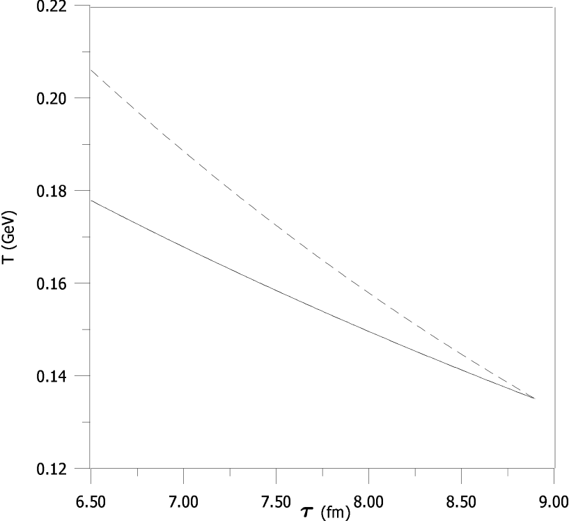
FIG. 3.: The temperature T (GeV) of the hadron resonance gas as function of the proper time $\tau$ (fm/c) of its evolution. Solid line corresponds to the semi-relativistic solution $T(\tau)$ of Eqs. (37) and (41). Dashed line describes $T(\tau)$ in completely non-relativistic picture of evolution of Boltzmann gases, Eqs. (39) and (44), with the same initial conditions. The effective mass of the mixture of non-relativistic Boltzmann gases is $m=\sum\kappa_{i}m_{i}\approx 0.662$ GeV.

One can restore the proper time of the chemical freeze-out from the intercept of the curve $T(\tau)$ at the temperature of the chemical freeze-out $T_{ch}\approx 163.37$ MeV, that was found from the analysis of particle number ratios. Using the result, $\tau_{ch}=7.24$ fm/c, one can calculate the effective volume $V_{eff}^{ch}\approx 2\pi\tau_{ch}R_{T}^{2}(\tau_{ch})\approx 975$ fm³ associated to unit of rapidity at mid-rapidity, and then find common chemical potential $\mu_{ch}$ from pion multiplicities at mid-rapidity, $dN_{\pi^{-}}/dy\approx 160$ [9]. For direct pions the common chemical potential $\mu_{ch}$ is added to phenomenological one: $\mu_{\pi,ch}=$ $\mu_{\pi}+\mu_{ch}$. Then one can easily evaluate the energy and particle densities.

Before proceeding to numerical results, let us check the validity of our basic approximations. The duration of hydrodynamic expansion of hadron gas, $\Delta\tau=8.9-7.24=1.66$ fm/c, is smaller or comparable with the relaxation time to chemical equilibrium in the system (see, e.g., [57, 58]), that exclude the chemical equilibration during the evolution. The typical life-time of the short lived resonances, is, however, compared with the period of hadron hydrodynamic stage $\Delta\tau=1.66$ fm/c, therefore, such decays could take place at the background of chemically non-equilibrium expansion. The decays could result in an increase of number of (quasi) stable particles during the expansion (without that all particle numbers will conserve within concept of chemical freeze-out). On the other hand, there are back reactions, that produce the resonances. These reactions do not lead to chemical equilibrium, but just reduce effect of resonance decays into the chemically non-equilibrium medium, resulting in an increase of effective life-time of resonances.

At the same time, some residual effect of resonance decays during the evolution could, anyway, take place. We ignore that effect since our approximate calculation of resonance decays demonstrate two opposite influences of it on a fluid evolution. (To do this estimate we replace the discrete spectra of heavy resonances by the Hagedorn distribution). The decay of heavier resonances with subsequent thermalization of decay products leads to a heating of the system, while the decay of relatively light resonances results in cooling. The reason is clear: the difference between kinetic energy of decay products and kinetic energy of thermal motion of the same particles (e.g. pions) is positive in the former case and negative in the latter one. Hence, the corresponding effects are approximately compensated and give no big influence on hydrodynamic evolution.

Our results are presented in Table 5. The first line corresponds to parameters at thermal freeze-out which are represented in the first line of Table 4. In Table 5 we present also our results for proper time and densities at the hadronization stage based on the thermal freeze-out parameters taken from other papers: fits 2-5 from Table 4.

From the results presented in Table 5 one can see that the ratio of energy density to total particle density at chemical freeze-out reaches the value $\varepsilon_{ch}/n_{ch}=0.997$ GeV, in agreement with the phenomenological observation in Ref. [6]. The energy density at the hadronization point $\overline{\varepsilon}_{ch}\approx 0.42$ GeV/fm³ is close to results of lattice calculation at the region of the phase transition and about equal to the energy density inside a nucleon. Note that for temperature and chemical potential found in [3] at the chemical freeze-out, we get $\overline{\varepsilon}_{ch}\approx 0.54$ GeV/fm³ and $\varepsilon_{ch}/n_{ch}\approx 1.16$ GeV, that is close to our results. Using the values of concentrations of HG and temperatures at chemical and thermal freeze-out, we get for conventional velocity of sound $c_{0}^{2}=p/\varepsilon=T/\sum\kappa_{i}e_{i}(T)$ the values $0.164$ and $0.145$ at chemical freeze-out and thermal freeze-out, respectively. Such relatively small values are determined by the large average mass of particles in hadron resonance gas, that is $0.662$ GeV for hadronic masses below $2$ GeV.

In Table 4 we list also the total particle number density $\overline{n}_{th}=\overline{n}_{ch}V_{eff}^{ch}/V_{eff}^{th}$, and chemical potential for direct pions $\mu_{\pi,th}$ at thermal freeze-out. One can see that for small temperature fits, $T_{th}=100\div 120$ MeV (fits 2 and 3) the chemical potential of direct pions at the stage of system decay seems to be too large and closed to condensation point, $\mu_{\pi,th}=m_{\pi}$.

Using Eqs. (56), (67) and velocity at Gaussian ”boundary” of the system at the chemical freeze-out $v_{R_{T}}(\tau_{ch})$$=$$\stackrel{{\scriptstyle.}}{{R}}_{T}(\tau_{ch})$, we calculate the averaged velocity at chemical freeze-out $\left\langle v\right\rangle_{ch}$ for fit $1$ and find that $\left\langle v\right\rangle_{ch}\approx 0.383$.

TABLE 5. The characteristics of the chemical freeze-out in Pb+Pb SPS collisions.

Fit	$\tau_{ch}$ fm	$\mu_{ch}$ MeV	$R_{T}(\tau_{ch})$ fm	$v_{R_{T}}(\tau_{ch})$$=$$\stackrel{{\scriptstyle.}}{{R}}_{T}(\tau_{ch})$	$\overline{\varepsilon}_{ch}$ GeV/fm3	$\overline{n}_{ch}$ 1/fm3
$1$	$7.24$	$-67$	$4.63$	$0.304$	$0.420$	$0.421$
$2$	$4.1$	$-9.8$	$5.18$	$0.278$	$0.598$	$0.600$
$3$	$4.2$	$-13.5$	$5.19$	$0.245$	$0.583$	$0.585$
$4$	$5.3$	$-76.1$	$5.55$	$0.240$	$0.398$	$0.399$
$5$	$4.8$	$-110.4$	$6.53$	$0.491$	$0.323$	$0.324$

VII Conclusions

The reconstruction of the hadronization stage for CERN SPS Pb+Pb collisions at 158A GeV/c is obtained within the hydrodynamic approach for the post-hadronization stage. Because of incomplete stopping at SPS energy we demonstrate that the analysis of particle ratios can be done within a relatively narrow rapidity window near mid-rapidity, provided one takes a non-uniformity in $\mu_{B}$ into account. We estimate that the non-uniformity of baryochemical potential may result in small but noticeable ($\approx 10$ $\%$) contribution to the pion multiplicity at mid-rapidity due to transport of pions from resonance decays from non-central rapidity regions. Using an optimization procedure for the calculation of particle number ratios near mid-rapidity, and also reconstructing the thermal freeze-out stage from spectra and correlations for different particle species, we find the physical conditions at the hadronization stage. The proper time for chemical freeze-out is found to be too small, $\tau_{ch}\approx 7.2$ fm/c to reach the chemical equilibrium in pure hadron gas, or cascade “event generator”, approach. We stress that our method does not assume complete chemical equilibrium of Boltzmann gases at the hadronization, and allow to estimate the deviation from it. We find that distribution functions of hadrons at hadronization hypersurface include some common factor, $\exp(\mu_{ch}/T_{ch})\approx 0.66$, that reduces essentially particle numbers as compare to chemically equilibrium ones. The energy density is found to be close to the results of lattice calculations at the point of the phase transition. The ratio of energy density to total particle number density is found to be about 1 GeV.

All those results indicate the existence of a pre-hadronic stage of expansion before the chemical freeze-out and the comparison with lattice calculations pointed to a QGP phase as most probable state of the matter till $\tau\simeq$ $7.2$ fm/c in Pb+Pb 158 A GeV/c collisions. The obtained characteristics of the hadronization give the possibility to make the next step and reconstruct the pre-hadronic stage of evolution and, then, to study the basic properties of  QGP.

REFERENCES

- [1] P.Braun-Munzinger, J.Stachel, J.P.Wessels, N.Xu, Phys. Lett. B 365, 1 (1996).
- [2] P.Braun-Munzinger, J.Stachel, J.P.Wessels, N.Xu, Phys. Lett. B 344, 43 (1995).
- [3] P.Braun-Munzinger, I.Heppe, J.Stachel, Phys. Lett. B 465, 15 (1999).
- [4] P.Koch, B.Muller, J.Rafelski, Phys. Rep. 142, 167 (1986); H.Bebie, P.Gerber, J.L.Goity, H.Leutwyler, Nucl. Phys. B 378, 95 (1992); J.Rafelski, J.Letessier, A.Tounsi, Acta Phys. Pol. B 27, 1037 (1996).
- [5] Yu.M.Sinyukov, S.V.Akkelin, A.Yu.Tolstykh, Nukleonika 43, 369 (1998).
- [6] J.Cleymans, K.Redlich, Phys. Rev. C 60, 054908 (1999).
- [7] J.Barrette et al, E877 Collaboration, Nucl. Phys. A 610, 153c (1996); L.Ahle et al, E866 Collaboration, Phys. Rev. C 57, R466 (1998); B.B.Back et al, (E917 Collab.), Phys. Rev. Lett. 86, 1970 (2001).
- [8] F.Shengqin, L.Feng, L.Lianshou, Phys. Rev. C 63, 014901 (2000)
- [9] F.Sikler for the NA49 Collaboration, Nucl. Phys. A 661, 45c (1999).
- [10] H.Appelshauser et al., (NA49 Collab.), Phys. Rev. Lett. 82, 2471 (1999).
- [11] A.Kostyuk, M.Gorenstein, H.Stocker, W.Greiner, Phys. Rev. C 63, 044901 (2001).
- [12] J.D.Walecka, Ann. Phys. 83, 491 (1974); Phys. Lett. B 59, 109 (1975); G.F.Bertch, S.Das Gupta, Phys. Rep. 160, 189 (1988).
- [13] J.Zimanyi, T.S.Biro, T. Csörgő, P.Levai, Phys. Lett. B 472, 243 (2000).
- [14] C.M.Hung, E.Shuryak, Phys. Rev. C 57, 1891 (1998).
- [15] S. Pratt, J. Murray, Phys. Rev. C 57, 1907 (1998).
- [16] S. Bass and A. Dumitru, Phys. Rev. C 61, 064909 (2000).
- [17] Yu.M.Sinyukov, S.V.Akkelin, Nu Xu, Phys. Rev. C 59, 3437 (1999).
- [18] B.Tomasik, U.A.Wiedemann, U.Heinz, nucl-th/9907096; U.A.Wiedemann, Nucl. Phys. A 661, 65c (1999).
- [19] A.Ster, T. Csörgő, B.Lörstad, Nucl. Phys. A 661, 419c (1999).
- [20] P.Braun-Munzinger, D.Magestro, K.Redlich, J.Stachel, Phys. Lett. B 518, 41 (2001).
- [21] P.Braun-Munzinger, J.Stachel, Nucl. Phys. A 606, 320 (1996).
- [22] R. Stock, Phys. Lett. B 456, 277 (1999).
- [23] D. Teaney, J. Lauret and E.V. Shuryak, nucl-th/0110037.
- [24] T. Hirano, K. Tsuda, nucl-th/0205043.
- [25] D. Teaney, nucl-th/0204023.
- [26] U. Heinz, P. Kolb, hep-ph/0111075; hep-ph/0204061.
- [27] F. Cooper, G. Frye, Phys. Rev. D 10, 186 (1974).
- [28] Yu.M. Sinyukov, S.V. Akkelin, Y. Hama, nucl-th/0201015, to be published in Phys.Rev.Lett. (2002).
- [29] D. Ferenc, Nucl. Phys. A 610, 523c (1996).
- [30] J.Sollfrank, Eur. Phys. J. C 9, 159 (1999).
- [31] L.D.Landau, Izv. Akad. Nauk SSSR, Ser. Fiz. 17, 51 (1953).
- [32] J.D.Bjorken, Phys. Rev. D 27, 140 (1983).
- [33] S. V. Akkelin, T. Csörgő, B. Lukács, Yu. M. Sinyukov and M. Weiner, Phys. Lett. B 505, 64 (2001).
- [34] R.Caliandro for the WA97 Collaboration, J. Phys. G: Nucl. Part. Phys. 25, 171 (1999).
- [35] C.Höhne for the NA49 Collaboration, Nucl. Phys. A661, 485c (1999).
- [36] L.Sandor for the WA97 Collaboration, talk at XXX International Symposium on Multiparticle Dynamics (ISMD 2000), Tihany, Hungary, 9-15 October 2000.
- [37] F.Sikler for the NA49 Collaboration, talk at XXX International Symposium on Multiparticle Dynamics (ISMD 2000), Tihany, Hungary, 9-15 October 2000.
- [38] M.Kaneta for the NA44 Collaboration, Nucl. Phys. A 638, 419c (1998).
- [39] S.V.Afanasiev et al., (NA49 Collab.), Phys. Lett. B 486, 22 (2000).
- [40] T.S.Biro, Phys. Lett. B 474, 21 (2000).
- [41] T.Csörgő, F.Grassi, Y.Hama, T.Kodama, hep-ph/0204300.
- [42] Stephen Wolfram, Mathematica Version 3.0, Wolfram Research, Inc. 1996.
- [43] S.V. Akkelin, Yu.M. Sinyukov, Z.Phys. C 72, 501 (1996).
- [44] U.A.Wiedemann, U.Heinz, Phys. Rev. C 56, 3265 (1997).
- [45] S.V. Akkelin, Yu.M. Sinyukov, Phys. Letters B 356, 525 (1995); Yu.Sinyukov, S.Akkelin, A.Tolstykh, Nucl. Phys. A 610, 278c (1996).
- [46] F. Antinori et al., (WA97 Collab.), Eur. Phys. J. C 14, 633 (2000).
- [47] A.N.Makhlin, Yu.M.Sinyukov, Z. Phys. C 39, 69 (1988); Yu.M.Sinyukov, Nucl. Phys. A 498, 151c (1989); Yu.M.Sinyukov, Nucl.Phys.A 566, 589c (1994); in: Hot Hadronic Matter: Theory and Experiment, eds. J.Letessier et al, (Plenum Publ. Corp., 1995), p. 309.
- [48] Yu.M.Sinyukov, talk at Int. Workshop “Particle interferometry in high energy heavy ion reactions”, ECT, Trento, September 1996 (unpublished).
- [49] J.Bolz, U.Ornik, M.Plümer, B.R. Schlei, and R.M. Weiner, Phys. Lett. B 300, 404 (1993); Phys. Rev. D 47, 3860 (1993); B.R. Schlei, U.Ornik, M.Plümer, D. Strottman and R.M. Weiner, Phys. Lett. B 376, 212 (1996).
- [50] R.Ganz for the NA49 Collaboration, Nucl. Phys. A 661, 448c (1999).
- [51] D.M.Reichholde for the NA44 Collaboration, Nucl. Phys. A 661, 435c (1999).
- [52] L. Conin, Ph.D. thesis, Paris, Orsay, 2001. See also at http://www.star.bnl.gov/~conin/these-all.ps.gz.
- [53] J. Bondorf, S. Garpman, J. Zimanyi, Nucl. Phys. A 296, 320 (1978).
- [54] K.S. Lee, U. Heinz, E. Schnedermann, Z. Phys. C 48, 525 (1990).
- [55] F.S. Navarra, M.S. Nemes, U. Ornik, and S. Paiva, Phys. Rev. C 45, 2552 (1992).
- [56] E. Schnedermann, U. Heinz, Phys. Rev. C 47, 1738 (1993).
- [57] Ch. Song, V. Koch, Phys. Rev. C 55, 3026 (1997).
- [58] R. Rapp, E. Shuryak, Phys. Rev. Lett. 86, 2980 (2001).