GRS computation of deep inelastic electron scattering on ⁴He

Abstract

We compute cross sections for inclusive scattering of high energy electrons on ⁴He, based on the two lowest orders of the Gersch-Rodriguez-Smith (GRS) series. The required one- and two-particle density matrices are obtained from non-relativistic ⁴He wave functions using realistic models for the nucleon-nucleon and three-nucleon interaction. Predictions for $E$=3.6 GeV agree well with the NE3 SLAC-Virginia data.

I Introduction

Total nuclear structure functions (SF) contain at least two components, namely one describing nuclei as composed of point-particles and a second one accounting for the internal structure of the nucleons. Since the latter are taken from experiment, a computation of total nuclear SF amounts to a determination of the same for a nucleus which is composed of point-particles. Such a calculation is usually performed within one of the following two approaches. In the first, one perturbatively expands the SF in the residual interaction between a nucleon struck by the virtual photon and the remaining spectator nucleus, thus generating the Impulse Series (IS) for the SF. In the widely used lowest order Impulse Approximation this residual interaction is first neglected. One then either computes higher order Final State Interaction (FSI) terms (see for instance Refs. [1, 2]), or models them [3, 4, 5, 6].

An alternative approach is based on a relativistic generalization of the Gersch-Rodriguez-Smith (GRS) expansion of SF in inverse powers of the 3-momentum transfer ${|{\mbox{\boldmath$q$}}|}$ [7, 8, 9]. Both theories have been applied to cross sections for inclusive scattering of high-energy leptons from various nuclear targets [3, 4, 5, 6, 10, 11].

When applied to high energy inclusive scattering one usually limits a GRS calculation to the two lowest order terms. Their determination requires knowledge of one- and two-particle density matrices, which are not diagonal in the coordinate of the struck nucleon ^′1^′, and of the spectral function. The non-diagonal one-body density matrix is related to the single-nucleon momentum distribution $n(p)$ and is usually extracted from alternative experimental sources, or is computed from theoretical models. There generally is no direct information on the half-diagonal, two-particle density matrices for finite systems and one relies on parametrizations [7, 12]. In those, nuclear recoil is usually neglected, thereby limiting applications to targets with $A\gtrsim 12$.

In the following we exploit accurately computed non-relativistic (NR) wave functions for light nuclei, using a number of modern realistic nucleon-nucleon ($NN$) and three-nucleon ($3N$) interactions. Those wave functions are Galilean invariant and enable a realistic GRS calculation of inclusive scattering on those nuclei. As a first application we choose ⁴He and for that target we shall report below predictions and a comparison with data.

The other ingredient, namely the ⁴He spectral function ${\cal P}(p,{\cal E})$, is rather difficult to compute and only a few direct calculations are reported [13, 14]. Below we shall adopt the reasonable alternative that has been developed by Ciofi degli Atti and Simula [6].

At this point we mention that for years the IS and GRS approaches have been considered as being distinct and even incompatible. Only recently has their equivalence been demonstrated, provided both series are expanded to the same order in the same parameter [2, 8, 9]. Following the derived prescription to link the two approaches, one can perform an interesting numerical comparison.

The GRS and IS theories are not the only tools which have been used to compute nuclear SF. We mention in particular the ingenious method of Efros and co-workers, which has been applied to ⁴He [14, 15]. Regrettably, it appears not feasible to extend that method to high energies.

The present note is organized as follows. In section II we recall the GRS approach, emphasizing the two main ingredients of our calculations, namely the SF of a target composed of point-particles and the SF of the free nucleons. We also discuss there the computation of the above density matrices. In section III we compare predictions for cross sections with the Virginia-SLAC data [16]. In the last section we present our conclusions.

II Total nuclear structure functions.

The cross section per nucleon for inclusive scattering of high-energy electrons from a nucleus with $A$ nucleons reads

$$\frac{d^{2}\sigma_{eA}(E;\theta,\nu)/A}{d\Omega\,d\nu}=\frac{2}{M}\sigma_{M}(E;\theta,\nu)\bigg{[}\frac{xM^{2}}{Q^{2}}F_{2}^{A}(x,Q^{2})+{\rm tan}^{2}(\theta/2)F_{1}^{A}(x,Q^{2})\bigg{]}\ ,$$ (1)

where $M$ is the nucleon mass, $\sigma_{M}$ the Mott cross section, $E$ the beam energy, $\theta$ the laboratory scattering angle and $\nu$ the energy loss imparted onto the target. The above nuclear structure functions per nucleon $F_{k}^{A}(x,Q^{2})$ contain the essence of unpolarized electron scattering from randomly oriented targets. Those SF depend on the squared 4-momentum transfer $-q^{2}=Q^{2}={\mbox{\boldmath$q$}}^{2}-\nu^{2}$ and on the Bjorken variable $x=Q^{2}/2M\nu$ with range $0\leq x\leq A$. For given beam energy $E,\,\,\,(\theta,\nu)$ and $(x,Q^{2})$ are sets of alternative kinematic variables.

Total nuclear structure functions per nucleon may, in a semi-heuristic fashion, be expressed as follows [17, 18, 19]

$$F^{A}_{k}(x,Q^{2})=\int_{x}^{A}\frac{dz}{z^{2-k}}f^{PN,A}(z,Q^{2})\sum_{l=1}^{2}C_{kl}({Q^{2}\over x^{2}},z)F_{l}^{\langle N\rangle}\bigg{(}\frac{x}{z},Q^{2}\bigg{)}\ ,$$ (2)

where $f^{PN,A}$ is the SF of a nucleus composed of point-particles and $F_{k}^{\langle N\rangle}$ is the averaged free nucleon SF. For a nucleus $A(Z,N)$

$$F_{k}^{\langle N\rangle}(x,Q^{2})={Z\over A}F^{p}_{k}(x,Q^{2})+{N\over A}F^{n}_{k}(x,Q^{2})\ ,\qquad k=1,2\ .$$ (3)

The coefficient functions $C_{kl}$ account for the mixing and modification of the free nucleon structure functions in the expression (2) [20]. We retained in this paper only the dominant coefficient

$$C_{22}({Q^{2}\over x^{2}},z) \approx [1-\rho+\rho/z]^{2}-{1\over 2}\rho(1-\rho)(1-1/z)^{2}\ ,$$ (4)

$$\rho = [1+Q^{2}/4M^{2}x^{2}]^{-1}\ .$$ (5)

Eq. (5) is a better approximation for $C_{22}$ than previously used [19].

Eq. (2) is valid for $x\gtrsim 0.15-0.20$, below which pionic and anti-screening effects become of importance [21] and above some critical $Q_{c}^{2}$, which presumably can be estimated using QCD. A previous comparison of predictions and data for medium-$A$ targets produced an empirical estimate $Q^{2}\gtrsim Q_{c}^{2}\approx 2.0-2.5\,$GeV²  [11].

Each of the SF $F^{p,n}_{k}$ in (2) has both nucleon-elastic (NE) and nucleon-inelastic (NI) parts, thus $F_{k}^{N}=F_{k}^{N,{\rm NE}}+F_{k}^{N,{\rm NI}}$, with $N=p,n$. The total nuclear structure functions, Eq. (2), and the total cross section per nucleon may therefore be expressed as a sum over contributions coming from the NE and NI parts of nucleon SF. In particular, the NE part $F_{k}^{N,{\rm NE}}$ is the well-known combinations of static electro-magnetic form factors and contributes primarily around the region of the quasi-elastic peak (QEP), $x\approx 1$. For the inelastic parts $F_{k}^{n,{\rm NI}}$ we have taken

$$F^{n,{\rm NI}}_{k}(x,Q^{2})\approx F_{k}^{d,{\rm NI}}(x,Q^{2})-F_{k}^{p,{\rm NI}}(x,Q^{2})\ ;\qquad k=1,2\ ,$$ (6)

where $F^{d,{\rm NI}}_{k}(x,Q^{2})$ are the deuteron SF’s per nucleon. For $F^{p,{\rm NI}}_{1}(x,Q^{2})$ and $F^{d,{\rm NI}}_{1}(x,Q^{2})$ we employ values interpolated between the data of Ref. [22], whereas for $F^{p,{\rm NI}}_{2}(x,Q^{2})$ and $F^{d,{\rm NI}}_{2}(x,Q^{2})$ we use the parametrizations of Ref. [23].

A The GRS series

We now focus on $f^{PN,A}$ in Eq. (2), the SF for a nucleus of point-particles, which has to be computed. Following Ref. [10] one writes

$$f^{PN,A}(x,Q^{2})=\left(\frac{\partial y_{G}}{\partial x}\right)_{Q^{2}\ {\rm fixed}}\phi({|{\mbox{\boldmath$q$}}|},y_{G})\ ,\qquad{|{\mbox{\boldmath$q$}}|}=Q\sqrt{1+\bigl{(}Q/2Mx\bigr{)}^{2}}\ ,$$ (7)

where $\phi({|{\mbox{\boldmath$q$}}|},y)$ is the reduced response in terms of a relativistic scaling variable [8]

$$y_{G}=y_{G}^{\Delta} \approx y_{G}^{\infty}\bigg{[}1-\frac{1}{2A^{\prime}}\frac{\nu^{2}}{{|{\mbox{\boldmath$q$}}|}^{2}}\xi+{\cal O}(1/A^{\prime 2})\bigg{]}\ ,\qquad A^{\prime}=A-1\ ,$$ (8)

$$y_{G}^{\infty} = \frac{M\nu}{{|{\mbox{\boldmath$q$}}|}}\xi\ ,$$ (9)

$$\xi = \bigg{(}1-\frac{\langle\Delta\rangle}{M}-x\bigg{)}\ ,$$ (10)

and $\langle\Delta\rangle$ some average nucleon separation energy. We shall retain the above $1/A^{\prime}$ correction in the scaling variable $y_{G}$ which, as Eq. (10) shows, is simply related to the Bjorken variable $x$. In the GRS approach the reduced response may, for smooth $NN$ interactions, be expanded in a series of inverse powers of ${|{\mbox{\boldmath$q$}}|}$ [7, 9]. Explicitly

$$\phi({|{\mbox{\boldmath$q$}}|},y_{G})=\phi_{0}({|{\mbox{\boldmath$q$}}|},y_{G})+\sum_{n\geq 1}\bigg{(}\frac{M}{{|{\mbox{\boldmath$q$}}|}}\bigg{)}^{n}\phi_{n}(y_{G})\ .$$ (11)

The lowest order term is given by

$$\phi_{0}({|{\mbox{\boldmath$q$}}|},y_{G}^{\Delta_{0}})=\int_{|y_{G}^{\Delta_{0}}|}^{\infty}\frac{dp\;p}{4\pi^{2}}\int_{0}^{E_{M}}d{\cal E}\;{\cal P}(p,{\cal E})+\theta(y_{G}^{\Delta_{0}})\int_{0}^{y_{G}^{\Delta_{0}}}\frac{dp\;p}{4\pi^{2}}\int_{E_{m}}^{E_{M}}d{\cal E}\;{\cal P}(p,{\cal E})\ ,$$ (12)

with ${\cal P}(p,{\cal E})$ the standard single-hole spectral function. The energy argument is ${\cal E}=E-\Delta_{0}$ with $E$ the removal energy and $\Delta_{0}$ the ($p,n$ averaged) minimal separation energy (for ⁴He $\Delta_{0}\approx 20.2$ MeV). Above, $y_{G}^{\Delta_{0}}$ is the scaling variable give in Eq. (10) with $\langle\Delta\rangle=\Delta_{0}$. The integration limits in (12) are

$$E_{M\atop m}(y_{G},p,{|{\mbox{\boldmath$q$}}|})=\frac{(y_{G}\pm p){|{\mbox{\boldmath$q$}}|}}{\nu}\ .$$ (13)

In actual calculations the spectral function has been written as in  Ref. [24]

$${\cal P}(p,{\cal E})=n_{0}(p)\delta({\cal E})+{\cal P}_{1}(p,{\cal E})\ ,$$ (14)

where $n_{0}(p)$ is the partial momentum distribution due to intermediate states of one nucleon and the $A-1$ spectator system in its ground state. Contributions from continuum states of that system are summed in ${\cal P}_{1}(p,{\cal E})$. As stated in the Introduction, that part of the spectral function for ⁴He has been taken to be ${\cal P}_{1}(p,{\cal E})={\cal N}(p){\cal P}^{\rm model}_{1}(p,{\cal E})$, where ${\cal P}^{\rm model}_{1}(p,{\cal E})$ has been provided by us by C. Ciofi degli Atti [6]. The normalization factor ${\cal N}(p)$ is fixed by

$$\int_{{\cal E}_{\rm thr}}^{\infty}d{\cal E}\;{\cal P}_{1}(p,{\cal E})=n(p)-n_{0}(p)\ ,$$ (15)

where the quantities $n(p)$, the total momentum distribution, and $n_{0}(p)$ have been calculated using the NR wave functions as will be explained in Subsect. II B.

We have also tested the following simple 2-state approximation for the spectral function [24, 15]

$${\cal P}(p,{\cal E})\approx n_{0}(p)\delta({\cal E})+[n(p)-n_{0}(p)]\delta({\cal E}-\langle\Delta\rangle+\Delta_{0})\ ,\qquad\langle\Delta\rangle\approx 50\ {\rm MeV}\ .$$ (16)

Substitution into (12) produces a ${|{\mbox{\boldmath$q$}}|}$-independent lowest order contribution,

$$\phi_{0}^{(1)}(y_{G}^{\Delta},y_{G}^{\Delta_{0}})=\frac{1}{4\pi^{2}}\bigg{[}\int_{|y_{G}^{\Delta}|}^{\infty}dp\,p\,n(p)-\int_{|y_{G}^{\Delta}|}^{|y_{G}^{\Delta_{0}}|}dp\,p\,n_{0}(p)\bigg{]}\ .$$ (17)

Since in the relevant $p$ region $n_{0}\approx n$, an accurate approximation of Eq. (17) reads

$$\phi_{0}^{(2)}(y_{G}^{\Delta_{0}})\approx\frac{1}{4\pi^{2}}\int_{|y_{G}^{\Delta_{0}}|}^{\infty}dp\,p\,n(p)\ .$$ (18)

Terms with $n\geq 1$ in Eq. (11) describe FSI corrections to the asymptotic limit as a series in $1/{|{\mbox{\boldmath$q$}}|}$. It is easier to give those in terms of their Fourier transform $\tilde{\phi}_{n}(s)$, namely

$$\phi_{n}(y_{G}^{\Delta})=\int_{0}^{\infty}{ds\over 2\pi}\;e^{isy_{G}^{\Delta}}\;\tilde{\phi}_{n}(s)\ .$$ (19)

Each $\tilde{\phi}_{n}(s)\equiv\tilde{\phi}_{n}(s;[V])$ is a functional of the bare interaction $V$, for instance

$$\frac{M}{{|{\mbox{\boldmath$q$}}|}}\tilde{\phi}_{1}(s) = \int d{\mbox{\boldmath$r$}}_{1}\int d{\mbox{\boldmath$r$}}_{2}\;\rho_{2}({\mbox{\boldmath$r$}}_{1},{\mbox{\boldmath$r$}}_{2};{\mbox{\boldmath$r$}}_{1}-s\hat{\mbox{\boldmath$q$}},{\mbox{\boldmath$r$}}_{2})[i\tilde{\chi}_{q}({\mbox{\boldmath$b$}},z;s)]\ ,$$ (21)

$$\tilde{\chi}_{q}({\mbox{\boldmath$b$}},z;s) = \tilde{\chi}_{q}^{(1)}({\mbox{\boldmath$b$}},z;s)+\tilde{\chi}_{q}^{(2)}({\mbox{\boldmath$b$}},z;s)\ ,$$ (22)

$$\tilde{\chi}_{q}^{(1)}({\mbox{\boldmath$b$}},z;s) = -\frac{M}{{|{\mbox{\boldmath$q$}}|}}\int_{0}^{s}d\sigma V({\mbox{\boldmath$b$}},z-\sigma)\ ,$$ (23)

$$\tilde{\chi}_{q}^{(2)}({\mbox{\boldmath$b$}},z;s) = \frac{M}{{|{\mbox{\boldmath$q$}}|}}sV({\mbox{\boldmath$b$}},z-s)=-s{\partial\over\partial s}\tilde{\chi}_{q}^{(1)}({\mbox{\boldmath$b$}},z;s)\ ,$$ (24)

where $b$ ($z$) is the component of the vector ${\mbox{\boldmath$r$}}={\mbox{\boldmath$r$}}_{1}-{\mbox{\boldmath$r$}}_{2}$ perpendicular (parallel) to the $q$ direction, and $\rho_{2}$ the semi-diagonal two-particle density matrix. Eqs. (19) define two parts of the off-shell eikonal phase $\tilde{\chi}_{q}$ which are related, and thus

$$\tilde{\chi}_{q}({\mbox{\boldmath$b$}},z;s)=\bigg{(}1-s{\partial\over\partial s}\bigg{)}\tilde{\chi}_{q}^{(1)}({\mbox{\boldmath$b$}},z,s)\ .$$ (25)

One frequently deals with interactions $V$ which have a strong short-range repulsion (or produce for other reasons a diffractive elastic amplitude) and it is then of advantage to perform a summation over a ladder of bare interactions $V$. The replacement $V\to V_{eff}=t_{q}$, produces a well-behaved, $q$-dependent, off-shell $t$-matrix as an effective interaction, which in coordinate space is proportional to the off-shell profile function $\tilde{\Gamma}$ [10]. For the part $\tilde{\Gamma}^{(1)}$, generated by $\tilde{\chi}^{(1)}$, one has

$$i\tilde{\chi}_{q}^{(1)}({\mbox{\boldmath$b$}},z;s) \to \tilde{\Gamma}^{(1)}_{q}({\mbox{\boldmath$b$}},z;s)={\rm exp}[i\tilde{\chi}_{q}^{(1)}({\mbox{\boldmath$b$}},z;s)]-1\ ,$$ (27)

$$\approx \theta(z)\theta(s-z)\Gamma_{q}^{(1)}(b)\ .$$ (28)

The approximation Eq. (28) has been tested in Ref. [25]. Its application permits the exploitation of a standard parametrization of the on-shell profile $\Gamma^{(1)}_{q}(b)$ in terms of elastic $NN$ scattering data, as are $\sigma_{q}^{tot},\tau_{q},Q^{(0)}_{q}$, which are respectively the total cross section, the ratio of the real to imaginary part of the forward elastic amplitude and the width of the diffractive amplitude. Explicitly,

$$\Gamma_{q}^{(1)}(b)\approx\frac{1}{2}\sigma_{q}^{tot}(1-i\tau_{q})\;{[Q^{(0)}_{q}]^{2}\over 4\pi}\;e^{-[bQ^{(0)}_{q}]^{2}/4}\ .$$ (29)

There is no simple way to generalize (25) to the total off-shell phase $\tilde{\chi}$. Yet as in [10] we shall assume that Eq. (25) is also approximately valid for the total off-shell profile function

$$i\tilde{\chi}_{q}({\mbox{\boldmath$b$}},z;s)\to\tilde{\Gamma}_{q}({\mbox{\boldmath$b$}},z;s) \approx \bigg{[}1-s{\partial\over\partial s}\bigg{]}\tilde{\Gamma}_{q}^{(1)}({\mbox{\boldmath$b$}},z;s)\ ,$$ (31)

$$\approx \bigg{[}1-s{\partial\over\partial s}\bigg{]}\theta(z)\theta(s-z)\Gamma_{q}^{(1)}(b)\ .$$ (32)

After substitution of the above expression in Eq. (19), the leading FSI contribution to $\tilde{\phi}({\mbox{\boldmath$q$}},s)$ turns into the following $q$-dependent result  [10]

$${M\over{|{\mbox{\boldmath$q$}}|}}\tilde{\phi}_{1}(s;[V])\to\frac{M}{{|{\mbox{\boldmath$q$}}|}}\tilde{\phi}_{1}(s,[t])=\tilde{G}_{1}({|{\mbox{\boldmath$q$}}|},s)=\tilde{G}_{1}^{(1)}({|{\mbox{\boldmath$q$}}|},s)+\tilde{G}_{1}^{(2)}({|{\mbox{\boldmath$q$}}|},s)\ ,$$ (33)

where

$$\tilde{G}_{1}^{(1)}({|{\mbox{\boldmath$q$}}|},s) \approx -\int d{\mbox{\boldmath$r$}}_{1}\int d{\mbox{\boldmath$r$}}_{2}\;\rho_{2}({\mbox{\boldmath$r$}}_{1},{\mbox{\boldmath$r$}}_{2};{\mbox{\boldmath$r$}}_{1}-s\hat{\mbox{\boldmath$q$}},{\mbox{\boldmath$r$}}_{2})\theta(z)\theta(s-z)\Gamma^{(1)}_{q}(b)\ ,$$ (35)

$$\tilde{G}_{1}^{(2)}({|{\mbox{\boldmath$q$}}|},s) \approx \int d{\mbox{\boldmath$r$}}_{1}\int d{\mbox{\boldmath$r$}}_{2}\;\rho_{2}({\mbox{\boldmath$r$}}_{1},{\mbox{\boldmath$r$}}_{2};{\mbox{\boldmath$r$}}_{1}-s\hat{\mbox{\boldmath$q$}},{\mbox{\boldmath$r$}}_{2})s\theta(z)\delta(s-z)\Gamma^{(1)}_{q}(b)\ .$$ (36)

Previous analyses dealt with targets with $A\geq 12$. For those there do not exist computations from first principles for single-nucleon momentum distributions $n_{0}(p)$, $n(p)$ and density matrices $\rho_{2}$, as required in (14), (15), (33). Moreover, suggested parametrizations [7, 12] do not account for nucleon-recoil, which is only justified for $A\gtrsim$ 12.

One of the predictions from Eq. (2) is a weak-$A$ dependence of the SF for point-nucleon nuclei and of the averaged nucleon SF [10]. This entails predicted inclusive cross sections per nucleon to be practically independent of $A$. Supporting evidence comes from experimental ratios of cross sections per nucleon for different targets at identical kinematical conditions [10, 11, 26]. Definitely larger deviations from smooth $A$-dependence are expected, if one of the targets is a light nucleus with $A\leq$6. This is evident from Table I where we entered some C/Fe ratios from JLab data  [27] and for He/C from the older NE3 data Ref. [16].

For the above reasons we did not include in the past a GRS analysis of inclusive scattering on the lightest targets. In the following we exploit the possibility to compute a precise NR nuclear ground state wave function $\Phi_{0}$ of light nuclei for given nuclear interaction $V$. Those enable a calculation of $n(p),n_{0}(p)$ and $\rho_{2}$, which enter the components (14), (15) and (33) of the nuclear SF.

B The density matrices

Various methods permit nowadays an accurate calculation of the ⁴He ground state wave function [28]. We exploit here the Correlated Hyperspherical Harmonic function (CHH) technique which has been developed by the Pisa group. The spatial configuration of the system is described in terms of a given choice of the Jacobi vectors ${\mbox{\boldmath$\xi$}}_{1},{\mbox{\boldmath$\xi$}}_{2},{\mbox{\boldmath$\xi$}}_{3}$. In the hyperspherical framework we use as new variables the hyperradius $\rho$, defined by

$$\rho^{2}=\sum_{i=1}^{3}\xi_{i}^{2}\ ,$$ (37)

and the set $\Omega=\{\hat{\xi}_{1},\hat{\xi}_{2},\hat{\xi}_{3},\varphi_{2},\varphi_{3}\}$. The latter includes the polar angles $\hat{\xi}_{i}\equiv(\theta_{i},\phi_{i})$ of each Jacobi vector and additional hyperspherical angles $\varphi_{2}$, $\varphi_{3}$. We then write for the ground state wave function $\Phi_{4}$

$$\Phi_{4}=\sum_{n=1}^{N_{tot}}\Bigg{[}{u_{n}(\rho)\over\rho^{4}}{\cal A}\biggl{\{}{\cal F}_{n}(r_{12},r_{13},r_{14},r_{23},r_{24},r_{34})\;{\cal Y}_{n}(\Omega)\biggr{\}}\Bigg{]}\ ,$$ (38)

where ${\cal A}$ is an anti-symmetrizer and ${\cal Y}_{n}(\Omega)$ are the four-body Hyperspherical Harmonic (HH) functions [29]. Choosing ${\cal F}_{n}=1$, Eq. (38) generates an uncorrelated HH expansion for the ⁴He ground state wave function. For it, the rate of convergence is extremely slow when the $NN$ interaction is strongly repulsive at small distances. One accounts for the latter property by multiplying every HH function in the expansion with a suitably chosen correlation factor ${\cal F}_{n}$, ultimately leading to the CHH expansion. The latter much improves the description of the target wave function for small inter-nucleon distances, and a much smaller number of basis functions is required to get convergence.

In the case of ⁴He, the correlation factors have been chosen to be of the Jastrow form [30]

$${\cal F}_{n}=f_{n}(r_{12})g_{n}(r_{13})g_{n}(r_{14})g_{n}(r_{23})g_{n}(r_{24})g_{n}(r_{34})\ ,$$ (39)

i.e. products of one-dimensional functions $f_{n}$ and $g_{n}$ which are solutions of a $NN$ Schrödinger-like equation (for details, see Ref. [30]).

Using the Rayleigh-Ritz variational principle for varying functions $u_{n}$ in (38)

$$<\delta_{u}\Phi_{4}|H-E|\Phi_{4}>=0\ ,$$ (40)

one is led to a set of hyperradial equations for the functions $u_{n}$ in the variable $\rho$ which, after discretization, is converted into a generalized eigenvalue problem and are solved by standard numerical techniques [31]. One thus determines the hyperradial functions $u_{n}(\rho)$ in Eq. (38) and the bound state energy $E$. We shall present below results based on

1) the Argonne V18 nucleon-nucleon (NN) potential [32] (the AV18 model),

2) the Argonne V18 NN potential supplemented by the Urbana IX three–nucleon potential [33] (the AV18UR model),

3) the Argonne V14 NN potential [34] plus the Urbana VIII three–nucleon potential [35] (the AV14UR model).

The two models, which contain a three-nucleon interaction provide a ⁴He binding energy rather close to the experimental one, whereas the AV18 under-binds by about 4 MeV. The present status of the ⁴He binding energy calculations with the CHH method is summarized in Table II, where in Eq. (38) up to $N_{tot}\approx 200$ functions have been used (the explicit CHH states included in the expansion are discussed in Ref. [30]).

Calculated binding energies for the AV18 or AV18UR Hamiltonians are within 1 % of the “exact” Green’s function Monte-Carlo (GFMC) results [33] for corresponding interactions. Somewhat less satisfactory agreement between the CHH and GFMC results for the AV14UR model, since this interaction is more repulsive at short distances than the other two. For all we checked that our final results for the deep inelastic scattering cross sections depend only slightly on the value of $N_{tot}$, once $N_{tot}\gtrsim 200$.

The thus constructed ground state wave function, readily gives the corresponding 4-body density matrices, in particular the one non-diagonal in ${}^{\prime}1^{\prime}$

$$\rho_{4}({\mbox{\boldmath$r$}}_{1},{\mbox{\boldmath$r$}}_{2},{\mbox{\boldmath$r$}}_{3},{\mbox{\boldmath$r$}}_{4};{\mbox{\boldmath$r$}}_{1}^{\prime},{\mbox{\boldmath$r$}}_{2},{\mbox{\boldmath$r$}}_{3},{\mbox{\boldmath$r$}}_{4})=\Phi_{4}({\mbox{\boldmath$r$}}_{1},{\mbox{\boldmath$r$}}_{2},{\mbox{\boldmath$r$}}_{3},{\mbox{\boldmath$r$}}_{4})\Phi_{4}({\mbox{\boldmath$r$}}_{1}^{\prime},{\mbox{\boldmath$r$}}_{2},{\mbox{\boldmath$r$}}_{3},{\mbox{\boldmath$r$}}_{4})$$ (41)

Successive integrations over the diagonal coordinates 3,4, and eventually over coordinate 2, then furnish $\rho_{2}$ and $\rho_{1}$ non-diagonal in ${}^{\prime}1^{\prime}$. The total momentum distribution is the Fourier transform of $\rho_{1}$.

The partial momentum distribution $n_{0}(p)$ is obtained from the overlap of $\Phi_{4}$ and the (³H, ³He averaged) three-nucleon ground state wave function $\Phi_{3}$, namely

$$n_{0}(p)=|a(p)|^{2}\ ,\qquad a(p)=\langle\;\Phi_{3}(1,2,3)\chi_{4}\eta_{4}|j_{0}(pR_{123,4})\Phi_{4}(1,2,3,4)\;\rangle\ ,$$ (42)

where $\chi_{4}$ ($\eta_{4}$) is the spin (isospin) state of particle 4, $j_{0}$ the zero-order Bessel function and $R_{123,4}$ the distance of particle 4 with respect to the center of mass of the other three. The ground state wave function $\Phi_{3}$ of the three-nucleon system has been obtained with the same Hamiltonian model used to generate $\Phi_{4}$, and again by application of the CHH technique [31]. In equation (42), $\Phi_{3}$ and $\chi_{4}\eta_{4}$ are coupled to give a state with vanishing total angular momentum and isospin.

Eqs. (33) for $\tilde{G}$ invite to express $\rho_{2}$ in terms of the variables ${\mbox{\boldmath$r$}}={\mbox{\boldmath$r$}}_{1}-{\mbox{\boldmath$r$}}_{2}$ and ${\mbox{\boldmath$R$}}=({\mbox{\boldmath$r$}}_{1}+{\mbox{\boldmath$r$}}_{2})/2$ and then to perform the $R$ integration

$$B({\mbox{\boldmath$b$}},z;s)=\int d{\mbox{\boldmath$R$}}\;\rho_{2}({\mbox{\boldmath$r$}}_{1},{\mbox{\boldmath$r$}}_{2};{\mbox{\boldmath$r$}}_{1}-s\hat{\mbox{\boldmath$q$}},{\mbox{\boldmath$r$}}_{2})$$ (43)

The result is substituted into (33) and subsequently integrated over $b$ and $z$.

C An effective IS series

In Ref. [3] one may find a detailed account of the lowest order PWIA calculations as part of the IS series. To it one should perturbatively add FSI due to the interaction of the knocked-out nucleon and the spectator core.

In the Introduction we recalled a recent proof [9, 2] that the GRS and IS, both evaluated to order ${\cal O}(1/{|{\mbox{\boldmath$q$}}|}^{2})$, produce the same result. The lowest order is given by

$$\phi_{0}({|{\mbox{\boldmath$q$}}|},y_{0})=\int_{|y_{0}|}^{2|{\mbox{\boldmath$q$}}|+y_{0}}\frac{dp\;p}{4\pi^{2}}\int_{0}^{{\bar{E}}_{M}}d{\cal E}\;{\cal P}(p,{\cal E})+\theta(y_{0})\int_{0}^{y_{0}}\frac{dp\;p}{4\pi^{2}}\int_{{\bar{E}}_{m}}^{{\bar{E}}_{M}}d{\cal E}\;{\cal P}(p,{\cal E})\ ,$$ (44)

where in this case [3, 9]

$${\bar{E}}_{M\atop m}=\sqrt{M^{2}+(y_{0}+{|{\mbox{\boldmath$q$}}|})^{2}}-\sqrt{M^{2}+(p\mp{|{\mbox{\boldmath$q$}}|})^{2}}\ .$$ (45)

Above, $y_{0}$ is the IS scaling variable defined by [3, 9]

$$y_{0} = y_{0}^{\infty}(1+\delta_{0})\ ,$$ (46)

$$y_{0}^{\infty} = -{|{\mbox{\boldmath$q$}}|}+\sqrt{(\nu-\Delta_{0})(\nu-\Delta_{0}+2M)}\ ,$$ (47)

$$\delta_{0} \approx -\frac{1}{2A^{\prime}}\bigg{[}\frac{1+\nu/M}{1+{|{\mbox{\boldmath$q$}}|}/y_{0}^{\infty}}\bigg{]}+{\cal O}(1/A^{\prime 2})\ .$$ (48)

The IS first order is then obtained from the prescription which puts $\tilde{G}_{1}^{(2)}=0$ in (33) and simultaneously replaces the GRS scaling variable $y_{G}^{\Delta}$, Eq. (10), by $y_{0}$ in Eq. (19). Finally, $f^{PN,A}(x,Q^{2})$ is now calculated using again $y_{0}$ in place of $y_{G}^{\Delta}$ in Eq. (7). Those changes have been shown to generate the IS series to order $1/{|{\mbox{\boldmath$q$}}|}$ [2]. Actual applications will be given in the following section.

III Results

In this section we present numerical results for inclusive cross sections on ⁴He based on Eqs. (1), (2). Unless stated differently, those results use density matrices based on the AV18UR interaction and the full spectral function as discussed in Sec. II A. In the GRS approach, the cross sections have been computed by approximating the reduced structure function as follows

$$\phi({|{\mbox{\boldmath$q$}}|},y_{G}) \to\phi_{0}({|{\mbox{\boldmath$q$}}|},y_{G}^{\Delta_{0}})\ ,\phantom{+G_{1}({|{\mbox{\boldmath$q$}}|},y_{G}^{\Delta_{0}})\equiv\phi_{01}({|{\mbox{\boldmath$q$}}|},y_{G}^{\Delta},y_{G}^{\Delta_{0}})} \qquad{\rm 0\ order}\ ,$$ (49)

$$\phi({|{\mbox{\boldmath$q$}}|},y_{G}) \to\phi_{0}({|{\mbox{\boldmath$q$}}|},y_{G}^{\Delta_{0}})+G_{1}({|{\mbox{\boldmath$q$}}|},y_{G}^{\Delta_{0}})\equiv\phi_{01}({|{\mbox{\boldmath$q$}}|},y_{G}^{\Delta_{0}})\ , \qquad{\rm 0+1\ order}\ ,$$ (50)

where $\phi_{0}$ is given by Eq. (12) and $G_{1}$ is the inverse Fourier transform of the functions given in Eq. (33). The corresponding IS expressions are obtained as discussed in Sect. II C.

In Fig. 1 we display the SLAC-Virginia NE3 cross section data [16] for $E$=3.595 GeV, scattering angles $\theta=$16^∘, 20^∘, 25^∘, 30^∘ and varying energy loss $\nu$, and also our numerical results obtained with the above reduced response $\phi_{01}$. Table III shows the ranges of the kinematical variables $x,\nu,Q^{2}$. For all measured scattering angle, and in addition for $\theta=45^{\circ}$, we entered there values of the energy loss $\nu$ and of $Q^{2}$ close to the appropriate lower ($x=2$) and upper ($x=0.1$) ends of the theoretical curves shown in Fig. 1. We also show the $\nu,Q^{2}$ values corresponding to the position of the QEP at $x=1$ .

Let us first focus on the NE part of the cross section (thin dashed lines), which contribute primarily around the QEP. As can be seen from the figure, the NE parts well describe the QEP, in particular at low $Q^{2}$. The data for $\theta=16^{\circ}$ show a clear maximum and an adjacent minimum which get fuzzier and ultimately disappear for increasing $\theta$ or $Q^{2}$. The same maximum occurs in the inclusive cross sections on deuterons [36], but is absent for targets with $A\geq 12$ [16, 27].

This structure is the result of the competition between the NE and the NI parts of the cross section. For decreasing $Q^{2}$ the NE part around the QEP $x=1$ grows relative to the, usually dominant, NI part. For the smallest $Q^{2}$ in the data, the NE part beyond the QEP stands out until for $x\lesssim 1$ the NI one overtakes. It is the maximum value of $f^{PN,A}(x,Q^{2})$ (for $x\approx 1$) which sets the magnitude of the QEP. For a given $Q^{2}$, that peak value decreases with $A$: it is largest for the deuteron and ⁴He and then it is almost independent on $A$ for $A\geq 12$, reflecting the smearing of the momentum distribution due to the Fermi motion. For example, $f^{PN,A}(x=1,Q^{2})$ for the deuteron and ⁴He is $\approx 5.5$ and $2.2$ times, respectively, larger than for nuclei with $A\geq 12$. It causes the QEP for equal kinematic conditions to be most prominent for the lightest nuclei.

We already mentioned that Eq. (2) (for the NI part) is estimated to be valid for $x\gtrsim 0.2$ and above some critical $Q_{c}^{2}\approx 2.0-2.5$ GeV² [10, 11]. As Table III shows, that approximate critical value is actually never reached for any $\theta=16^{\circ},20^{\circ}$ data point, which renders those data not really suitable for a test of the theory. For the same reason we excluded from our analysis NE3 data at lower energies and the same is the case for old, near-elastic, high-$Q^{2}$ data on ⁴He [37]. For both angles, the convolution formula predicts too large NI parts around the QEP, resulting in an over prediction of the data in that region. For $\theta=30^{\circ}$, on the other hand, $Q^{2}\gtrsim Q_{c}^{2}$ and, in fact, comparison of data and predictions shows that there is good agreement for all but the smallest energy loss values. Since cross sections there have fallen by orders of magnitude, one expects sensitivity to small dynamical details. For example, without the inclusion in Eq. (2) of the mixing factor $C_{22}$, Eq. (5), the agreement would be of definitely lower quality (see also below).

A more stringent test for the theory would be provided by data at higher beam energies with, in general, higher $Q^{2}$. Unfortunately, the recent 4 GeV experiments at JLab for various targets did not contain ⁴He [27], but a recent JLab proposal includes that target in a 6 GeV run with scattering angles $\theta=15^{\circ}$, $23^{\circ}$, $30^{\circ}$, $45^{\circ}$ and $60^{\circ}$ [38]. The kinematical region explored by that experiment covers $0.2<x<1.0$ and $1<Q^{2}<8.0$ GeV² (Table IV) and predictions for the four largest scattering angles can be found in Fig. 2. Incidentally, we checked that for $E=6$ GeV the effect of $C_{22}$ is practically negligible due to $Q^{2}$, which grows with beam energy $E$.

Next we discuss the effect of the different approximations for $\phi_{0}$ presented in Sec. II. The cross sections calculated using the approximations (17) and (18) for $\phi_{0}$ almost overlap. Moreover, they are rather similar to the ones computed using the spectral function, Eq. (12), except in the low $\nu$ region. There, the use of the “full” model slightly reduces the cross sections.

This result deserves some comment. The differences between the two expressions, Eqs. (12) and (18) are generally sizeable in particular in the low $\nu$ region [3] where $y_{G}^{\Delta_{0}}$ is negative and large in absolute value. However, in the kinematical region of the NE3 experiment, the values of $E_{M}$ entering Eq. (12) are found to be rather large and then

$$\int_{0}^{E_{M}}d{\cal E}{\cal P}(p,{\cal E})\approx\int_{0}^{\infty}d{\cal E}{\cal P}(p,{\cal E})=n(p)\ .$$ (51)

As a result, the $\phi_{0}$ calculated using Eqs. (12) or (18) nearly coincide. For example, for $E=3.595$ GeV, $\theta=30^{\circ}$ and $\nu=0.7$ GeV, ${|{\mbox{\boldmath$q$}}|}/\nu\approx 3$ and $E_{M}$ is large for all the values of $p$. For the same reason we expect that the predicted cross sections do not much depend on the parametrization chosen for the spectral function, in particular not in the low $\nu$ region. In that region they are rather sensitive to the tail of the momentum distributions, which in turn is related to the correlations in the nuclear wave functions [39].

In Fig. 3a we display the separate contributions of the cross sections at $E=3.595$ GeV, $\theta=30^{\circ}$ and varying $\nu$, as due to the NE and NI components of the nucleon SF $F_{k}^{\langle N\rangle}$. The thin (heavy) dashes are NE part in the $\phi_{0}$ ($\phi_{01}$) approximation for the reduced response. Those have their maximum at $x\approx 1$, and are only in the wings marginally affected by the 1st order FSI terms. The thin and heavy solid lines show the corresponding NI parts, which by nature dominate the region $x\lesssim 1$ for relatively high $\nu$. FSI affect only the low $\nu$ region and cause a rather small increase in cross sections. In those $\nu$-regions NE and NI parts are of the same order. Fig. 3b is as Fig. 3a for $\theta=45^{\circ}$ (this angle was chosen since the $Q^{2}$ values are larger and similar to those for $E=6$ GeV, $\theta=15^{\circ}$). The results are similar, except that FSI now appear to decrease the 0th NI contribution at low $\nu$.

From Fig. 3a we observe that the slight over-prediction in the low $\nu$ region of the theoretical results at $\theta=30^{\circ}$ is mainly due to the NI part and as discussed above, is only marginally affected by the inclusion of FSI. The reason of the large NI contribution can be simply understood by looking at the convolution (2) between the nucleon SF and $f^{PN,A}$.

Typical behavior of the functions $f^{PN,A}(z,Q^{2})$, $F^{\langle N\rangle,NI}_{2}(x/z,Q^{2})$ and the mixing factor $C_{22}(Q^{2}/x^{2},z)$, (the latter two for $x=0.1,2.0$) are given in Fig. 4 ($F^{\langle N\rangle,NI}_{1}$ behaves similarly). For $x<1$, the permitted range of values $z\geq x$ covers the $z\approx 1$ region where $f^{PN,A}(z,Q^{2})$ is large and allows virtually the entire support $x/z$ of $F^{\langle N\rangle,NI}$ to contribute. In contrast, for $x>1$ (see Fig. 4b), only the tail of $f^{PN,A}$ contributes and $F^{\langle N\rangle,NI}(t,Q^{2})$ for $x/A\leq t\leq 1$ is usually small. Moreover, $f^{PN,A}$ decreases as $z\rightarrow 4$. In fact, as $z$ becomes larger, also $|y_{G}^{\Delta_{0}}|$ increases and the integral in Eq. (12) decreases. However, $y_{G}^{\Delta_{0}}\approx-{\sqrt{Q^{2}}}/2$ for $z\gg 1$ and since the values of $Q^{2}$ in the $E=3.595$ GeV NE3 experiment are not large, $\phi_{0}$ and the corresponding $f^{PN,A}$ are still non-vanishing at $z\rightarrow 4$. As a consequence, the integrals receive a sizeable contribution from the region $z>3$ and the NI cross section in the low $\nu$ region remains large.

Note also that the mixing factor $C_{22}\approx 1$ for $x=0.1$ (Fig. 4a) but becomes rather small for $x=2$ (Fig. 4b), sizeably reducing the NI part of the cross section in that region. As stated before, without the inclusion of such a factor $C_{22}$, the over-prediction of the theoretical cross section in the low $\nu$-region would be more pronounced.

Next, applying the prescription recalled in subsection II C, we make a comparison between GRS and IS cross sections for $E=3.595$ GeV. Fig. 5a (5b) shows the results for $\theta=30^{\circ}$ using the $\phi_{0}$ ($\phi_{01}$) approximation for the reduced response, together with the NE3 data. The agreement between the two predictions is good, but not perfect. One of the causes is undoubtedly the use of (II A), which is an approximation for the parametrized, off-shell total profile function $\tilde{\Gamma}$, and is of course not intrinsic to the actual ladder summation. Also the agreement with the data is good, except for the smallest $\nu$.

One observes that the GRS and IS predictions using only $\phi_{0}$ diverge for decreasing $\nu$ and that the GRS prediction is closest to the data. This is shown in Fig. 5a for $\theta=30^{\circ}$, $E=3.595$ GeV, but holds in fact for all examined cases. Comparison of Figs. (5a) and (5b) moreover shows that FSI for GRS are smaller than for the IS, in particular for smaller $\nu$. The two observations above can be understood theoretically [9] and have previously been demonstrated for simple models.

Finally, one infers from Fig. 5b that the differences between the 0 order IS and GRS cross sections are noticeably reduced when the first order FSI is included in both calculations. A similar comparison is shown in Figs. 5c and 5d for $\theta=45^{\circ}$ and again the agreement is found to be good after the inclusion of the FSI.

The separate IS NE and NI parts for $E=3.595$ GeV and $\theta=30^{\circ}$ ($\theta=45^{\circ}$) are shown in Fig. 6a (Fig. 6b), where we used the same notation adopted in Fig. 3. In this case, the NI part computed with the $\phi_{0}$ approximation for the reduced response (thin solid line) stays well below the NE one (thin dashed line) in the low $\nu$ region, as already found in Ref. [3]. Now, in the evaluation of the convolution (2), $|y_{0}|$ becomes rather large as $z\rightarrow 4$ and $\phi_{0}$ rapidly decreases ($y_{0}\rightarrow-\sqrt{Q^{2}}$ as $z\gg 1$). As a consequence, the IS integrand of Eq. (2) is very small in the low $\nu$ region (in contrast to what happens in the GRS case). However, as already discussed in relation with Fig. 5, there the FSI contributions in the IS case are sizeable. In fact, now the FSI are given by Eq. (33) without the term $\tilde{G}^{(2)}_{1}$, which otherwise would partially cancel the contribution of the large term $\tilde{G}^{(1)}_{1}$. As a result, in the low $\nu$ region, the IS NI cross section calculated at the level of the 0+1 order becomes larger than the NE one, and rather close to the GRS NI cross section.

Another interesting aspect is the influence of the nuclear interaction, chosen to calculate the density matrices. In Fig. 7 we display for $E=3.595$ GeV, $\theta=30^{\circ}$ cross sections computed on the basis of the three previously mentioned models of nuclear interaction (AV18UR, AV18 and AV14UR). The calculations have been performed using $\phi_{0}$ from Eq. (18) with the density matrices determined directly from the corresponding nuclear wave functions. For identical kinematics the predictions for AV18UR and AV14UR can hardly be distinguished, whereas the AV18 cross section is slightly different from the other two in the low-$\nu$ tail: There clearly is only weak dependence on the nuclear interaction.

IV Conclusions

We have studied inclusive scattering of high-energy electrons from ⁴He, for energy losses below and around the quasi-elastic peak and up into the deep inelastic scattering region. The underlying model assumes non–interference between nucleonic and sub-nucleonic degrees of freedom, which implies that total nuclear structures function may be expressed as a generalized convolution of the structure functions of free nucleons and the one of a nucleus composed of point particles. The model is estimated to become gradually imprecise for $Q^{2}\lesssim 2-2.5$ GeV². Structure functions for a nucleus of point-particles are computed via the reduced response $\phi(q,y)$ using a relativistic generalization of the GRS series, which includes the first order FSI.

A new element in the development of the latter is an actual calculation of the required single- and two-particle, semi-diagonal density matrices, based on accurately computed ⁴He ground state wave function. The above replaces previously used parametrizations of derived density matrices for targets with $A\geq$ 12. Computed cross sections appear to be hardly dependent on the choice of the $NN$ interaction.

We also exploited a prescription to derive from the GRS series to order $1/q$ similar terms for the IS. The two methods produce cross sections which are rather similar, in particular after the inclusion of the corresponding FSI contributions.

In conclusion our predictions are in good agreement with the NE3 SLAC-Virginia data for all scattering angles, in spite of the fact that for $\theta\lesssim 30^{\circ}$ the involved $Q^{2}$ fall below the validity estimate. We also computed cross sections for a future JLab experiment at $E=6$ GeV. Its kinematics are largely within the estimated limits of the underlying theory and a comparison of theory with data will be more significant for those than is the case for the NE3 data.

V Acknowledgment

The authors are grateful for having received from C. Ciofi degli Atti tables of numerical values of the ⁴He spectral function, mentioned in Section II. One of us (M.V.) also gratefully acknowledges a helpful discussion with G.I. Lykasov.

FIG. 1.: Predicted cross sections for inclusive scattering of 3.595 GeV electrons from ⁴He as function of the energy loss $\nu$ and for four values of the scattering angles $\theta$ in the (0+1)th order approximation (thick solid lines). Thin dashed (solid) lines show the NE (NI) part of the cross sections. Data are from Ref. [16].

FIG. 2.: Predicted cross sections for inclusive scattering of 6.0 GeV electrons from ⁴He as function of the energy loss $\nu$ and for four values of the scattering angles $\theta$ in the (0+1)th order approximation (thick solid lines). Thin dashed (solid) lines show the NE (NI) part of the cross sections.

FIG. 3.: (a) Contributions to the cross section for $E=3.595$ GeV, $\theta=30^{\circ}$ from the NE (dashes) and the NI (solid lines) parts of the nucleon SF. Thin and thick lines are computed from the the 0th and (0+1)th order reduced response $\phi({|{\mbox{\boldmath$q$}}|},y_{G})$, respectively. The density matrices correspond to the AV18UR nuclear interaction. (b) The same as in (a), but for $\theta=45^{\circ}$.

FIG. 4.: The GRS function $f^{PN,A}(z,Q^{2})$ (thin solid line), the nucleon SF $F^{\langle N\rangle,{\rm NI}}_{2}(x/z,Q^{2})$ (long dashed line) and the mixing factor $C_{22}(Q^{2}/x^{2},z)$ (short dashed line) entering Eq. (2) as function of $z$ for $E=3.595$ GeV, $\theta=30^{\circ}$ and two cases of $x$: (a) $x=0.1$ (corresponding to have $Q^{2}=0.58$ GeV², $\nu=3.00$ GeV) and (b) $x=2$ ($Q^{2}=2.76$ GeV², $\nu=0.74$ GeV). $I(z)$ is the corresponding integrand of Eq. (2).

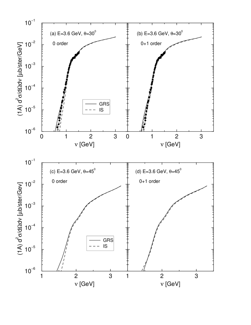
FIG. 5.: (a) Comparison of the 0th order GRS and derived IS cross sections for $E=3.595$ GeV, $\theta=30^{\circ}$. (b) As in (a) but in the case of the (0+1)th order. (c) and (d): as in (a) and (b), respectively, but for $\theta=45^{\circ}$.

FIG. 6.: As in Fig. 3 but for the IS case. (a) Contributions to the cross section for $E=3.595$ GeV, $\theta=30^{\circ}$ from the NE (dashes) and the NI (solid lines) parts of the nucleon SF. Thin and thick lines are computed from the the 0th and (0+1)th order reduced response $\phi({|{\mbox{\boldmath$q$}}|},y_{0})$, respectively. The density matrices correspond to the AV18UR nuclear interaction. (b) The same as in (a), but for $\theta=45^{\circ}$.

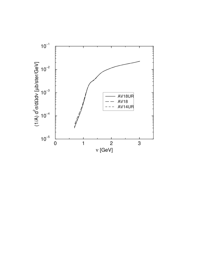
FIG. 7.: (0+1)th order GRS cross sections at $E=3.595$ GeV and $\theta=30^{\circ}$ for the AV18 (dashed), AV14UR (long dashed) and AV18UR (solid) nuclear interactions.

TABLE I.: Selection of cross section ratios He/C, C/Fe. For given angle we give $x,Q^{2}$ and the ratios. Former are from Ref.  [16], latter from Ref. [11].

$\theta=20^{\circ}$			$\theta=25^{\circ}$			$\theta=30^{\circ}$
$x$	$Q^{2}$	He/C	$x$	$Q^{2}$	He/C	$x$	$Q^{2}$	He/C
2.69	1.44	0.64	2.10	2.07	0.64	1.37	2.51	0.66
1.40	1.34	0.70	1.23	1.88	0.69	1.08	2.35	1.17
0.70	1.18	0.88	1.37	2.51	0.96	0.81	2.12	1.03

$\theta=15^{\circ}$			$\theta=30^{\circ}$
$x$	$Q^{2}$	C/Fe	$x$	$Q^{2}$	C/Fe
2.49	1.05	0.82	1.95	3.38	0.70
1.02	0.97	1.18	1.37	3.09	0.98
0.65	0.91	0.97	1.01	2.79	1.04
0.43	0.83	1.00	0.72	2.43	1.00

TABLE II.: Binding energies in MeV of ⁴He calculated with the CHH method using the AV18 and AV18/UIX, and the older AV14 and AV14/UVIII, Hamiltonian models. Also listed are the corresponding “exact”GFMC results [33] as well as the experimental value.

Model	CHH	GFMC
AV18	24.0	24.1(1)
AV18/UIX	28.1	28.3(1)
AV14	24.0	24.2(2)
AV14/UVIII	27.5	28.3(2)
EXP	28.3

TABLE III.: Values of $\nu$ (in GeV) and $Q^{2}$ (in GeV²) for $E=3.6$ GeV [16]. The selected values of $x$ correspond approximately to the QEP and the lower and upper ends of the curves shown in Fig. 1.

	lower end		QEP		upper end
	$x=2$		$x=1$		$x=0.1$
$\theta$	$\nu$	$Q^{2}$	$\nu$	$Q^{2}$	$\nu$	$Q^{2}$
$16^{\circ}$	0.25	0.93	0.46	0.87	2.00	0.44
$20^{\circ}$	0.37	1.40	0.68	1.27	2.50	0.48
$25^{\circ}$	0.55	2.06	0.95	1.79	2.80	0.54
$30^{\circ}$	0.74	2.76	1.22	2.29	3.00	0.58
$45^{\circ}$	1.23	4.99	1.90	3.58	3.31	0.62

TABLE IV.: Values of $\nu$ (in GeV) and $Q^{2}$ (in GeV²) for $E=6.0$ GeV and the values of $\theta$ of the proposed CEBAF experiment. The selected values of $x$ correspond approximately to the QEP and the lower and upper ends of the curves shown in Fig. 2.

	lower end		QEP		upper end
	$x=2$		$x=1$		$x=0.1$
$\theta$	$\nu$	$Q^{2}$	$\nu$	$Q^{2}$	$\nu$	$Q^{2}$
$23^{\circ}$	1.21	4.56	2.02	3.80	5.01	0.94
$30^{\circ}$	1.80	6.75	2.77	5.20	5.37	1.01
$45^{\circ}$	2.90	10.90	3.91	7.34	5.70	1.07
$60^{\circ}$	3.69	13.86	4.57	8.58	5.82	1.09

REFERENCES

- [1] N.N. Nikolaev, J. Speth and B.G. Zakaharov, J. Exp. Theor. Phys. 82, 1046 (1996); A. Bianconi, S. Jeshonnek, N.N. Nikolaev and B.G. Zakaharov, Phys. Lett. B 343, 13 (1995)
- [2] A.S. Rinat, B. K. Jennings, Phys. Rev. C59, 3371 (1999)
- [3] See for instance: C. Ciofi degli Atti, E. Pace and G. Salmè, Phys. Rev. C 43, 1155 (1991); C. Ciofi degli Atti, D.B. Day and S. Liuti, Phys. Lett. B 225, 215 (1989), Phys. Rev. C46, 1045 (1992)
- [4] O. Benhar, A. Fabrocini, S. Fantoni, G.A. Miller, V.R. Pandharipande and I. Sick, Phys. Rev. C44, 2328 (1991); Phys. Lett. B 359, 8 (1995)
- [5] P. Fernandez de Cordoba, E. Marco, H. Mutter, E. Oset and A. Faessler, Nucl. Phys. A611, 514 (1996)
- [6] C. Ciofi degli Atti and S. Simula, Phys. Lett. B 325, 276 (1994)
- [7] H. Gersch, L.J. Rodriguez and Phil N. Smith, Phys. Rev. A5, 1547 (1973)
- [8] S.A. Gurvitz, Phys. Rev. C42, 2653 (1990)
- [9] S.A. Gurvitz and A.S. Rinat, nucl-th/0106032; submitted to Phys. Rev. C.
- [10] A.S. Rinat and M.F. Taragin, Nucl. Phys. A598, 349 (1996); A620, 412 (1997); Erratum A623, 773 (1997)
- [11] A.S. Rinat and M.F. Taragin, Phys. Rev. C60, 044601 (1999)
- [12] A.S. Rinat, Phys. Rev. B40, 6625 (1989); A.S. Rinat, M.F. Taragin, F. Mazzanti and A. Polls, Phys. Rev. B57, 5347 (1998)
- [13] H. Morita and T. Suzuki, Progr. Theor. Phys. 86, 671 (1991)
- [14] V.D. Efros, W. Leidemann and G. Orlandini, Phys. Rev. C 58, 582 (1998)
- [15] V.D. Efros, W. Leidemann and G. Orlandini, Phys. Lett. B 338, 130 (1994); Phys. Rev. Lett. 78, 432 (1997)
- [16] D.B. Day , Phys. Rev. C48, 1849 (1993)
- [17] S.A. Gurvitz and A.S. Rinat, TR-PR-93-77/ WIS-93/97/Oct-PH; Progress in Nuclear and Particle Physics, Vol. 34, 245 (1995)
- [18] A.S. Rinat, Proceedings of the Second International Conference on ’Perspectives in Hadronic Physics’, ICTP, Trieste, Italy (1999), S. Boffi et al Eds., World Scientific (Singapore), p.62
- [19] A.S. Rinat and M.F. Taragin, Phys. Rev. C62, 034602 (2000)
- [20] G.B. West, Ann. of Phys. (NY) 74, 646 (1972); W.B. Atwood and G.B. West, Phys. Rev. D7, 773 (1973)
- [21] C.H. Llewellyn Smith, Phys. Lett. B 128, 117 (1983); M. Ericson and A.W. Thomas, Phys. Lett. B 128, 120 (1983)
- [22] A. Bodek and J.L. Ritchie, Phys. Rev. D23, 1070 (1981)
- [23] P. Amadrauz , Phys. Lett. B295, 159 (1992); M. Arneodo B364, 107 (1995)
- [24] C. Ciofi degli Atti and S. Simula, Phys. Rev. C53, 1689 (1996)
- [25] A.S. Rinat and M.F. Taragin, Nucl. Phys, A623, 519 (1997)
- [26] J. Arrington , Phys. Rev. C53, 2248 (1996)
- [27] J. Arrington , Phys. Rev. Lett. 82, 2056 (1999)
- [28] H. Kamada , Phys. Rev. C64, 044001 (2001)
- [29] M. Fabre de la Ripelle, Ann. Phys. (N.Y.) 147, 281 (1983)
- [30] M. Viviani, A. Kievsky and S. Rosati, Few–Body Systems 18, 25 (1995)
- [31] A. Kievsky, S. Rosati, M. Viviani, Nucl. Phys. A577, 511 (1994)
- [32] R.B. Wiringa, V.G.J. Stoks, and R. Schiavilla, Phys. Rev. C51, 38 (1995)
- [33] B.S. Pudliner et al., Phys. Rev. C56, 1720 (1997)
- [34] R.B. Wiringa, R.A. Smith, and T.L. Ainsworth, Phys. Rev. C29, 1207 (1984)
- [35] R. B. Wiringa, Phys. Rev. C43, 1585 (1991)
- [36] J. Arrington, private communication; I. Niculescu , Phys. Rev. Lett. 85, 1182 (2000)
- [37] S. Rock , Phys. Rev. 26, 1592 (1982)
- [38] J. Arrington (spokesperson) et al., “A Precise Measurement of the Nuclear Dependence of Structure Functions in Light Nuclei”, Jefferson Lab. Proposal E-00-101, May 2000
- [39] See, for instance, O. Benhar, S. Fantoni and G. I. Lykasov, Eur. Phys. J. A5, 137 (1999) and references therein.