What is the Correct $\pi^{-}p\rightarrow\omega n$ Cross Section at Threshold?

Abstract

The $\pi^{-}p\rightarrow\omega n$ threshold cross section of refs. binnie ; keyne ; karami resisted up to now a consistent theoretical description in line with experiment, mainly caused by too large Born contributions. This led to a discussion in the literature about the correctness of the extraction of these data points. We show that the extraction method used in these references is indeed correct and that there is no reason to doubt the correctness of these data.

I Introduction

In the 70’s a series of experiments binnie ; keyne ; karami was performed to measure the $\pi^{-}p\rightarrow\omega n$ cross section just above threshold. These data resisted up to now a consistent theoretical description, mainly caused by too large Born contributions klingl . As a consequence these diagrams were either neglected post ; friman or suppressed by very soft formfactors titov . These findings motivated a discussion in the literature about the experimentalists’ way to extract the two-body cross section hanhart99 and readjustments of the published $\pi^{-}p\rightarrow\omega n$ cross section data were performed sibi ; titov ; hanhart01 .

The cause of the discussion is the experimentalists’ unusual method to cover the full range of the $\omega$ spectral function. An integration over at least one kinematical variable is necessary to make sure that all pion triples with invariant masses around $m_{\omega}$ are taken into account, so that the $\omega$ spectral function with a width of $8$ Mev is well covered. Instead of fixing the incoming pion momentum and integrating out the invariant mass of the pion triples directly, the authors of binnie ; keyne ; karami fixed the outgoing neutron laboratory momentum and angle and performed an integration over the incoming pion momentum.

Led by the observation that the cross sections of binnie ; keyne ; karami result in a hard-to-understand energy dependence of the transition matrix element the authors of hanhart99 claimed that due to the experimental method just described the count rates covered only a fraction of the $\omega$ spectral function. As a consequence, the authors of hanhart99 ; sibi ; titov advocated that the two-body total cross sections given in karami ; landolt should be modified. Imposing this modification of the threshold cross section, in hanhart99 a practically constant transition matrix element up to $1.74$ GeV corresponding to an $S_{11}$ or $D_{13}$ hanhartprivate (since the pion momentum is almost constant in this region) wave production mechanism (in the usual $\pi N$ notation, i.e. an $IJ^{P}=\frac{1}{2}\frac{1}{2}^{-}$ or $IJ^{P}=\frac{1}{2}\frac{3}{2}^{-}$, resp., partial wave) was deduced.

This modification, however, immediately raises another problem. Taking into account this “spectral function correction” increases the $\omega N$ cross section for $1.72\leq\sqrt{s}\leq 1.74$ up to $\sigma\geq 3$ mb, which is in contradiction to the inelasticity deduced from $\pi N\rightarrow\pi N$ partial wave analyses (e.g. SM00 SM00 ). As can be seen in fig. 1

Figure 1: $S_{11}$ inelastic partial wave cross section of $\pi N\rightarrow\pi N$ as deduced from SM00 SM00 $\circ$ and $\pi N\rightarrow 2\pi N$ partial wave cross section as deduced by manley $\bullet$. The curve gives the result of a coupled-channel analysis moretocome .

the $\pi N\rightarrow\pi N$ inelasticity in the $S_{11}$ partial wave is already saturated by $\pi N\rightarrow 2\pi N$ in this energy region, i.e. an additional $\omega N$ contribution of $\sigma^{S_{11}}\geq 3$ mb would lead to a gross overestimate of the inelasticity:

$$\sigma^{S_{11}}_{in} \geq \sigma^{S_{11}}_{2\pi N}+\sigma^{S_{11}}_{\omega N}$$ (1)

$$\geq 2.5\;\mathrm{mb}+3\;\mathrm{mb}\gg 2.4\;\mathrm{mb}\approx\sigma^{S_{11}}_{in}(\mathrm{SM00})\;.$$

The same argument holds for the $D_{13}$ wave (see fig. 5 in moretocome ).

Because of this inconsistency of the newly extracted cross sections with existing inelasticities and because of the importance of the $\pi N\rightarrow\omega N$ cross section for both unitary models analyzing reactions on the nucleon in the c.m. energy range $1.7\leq\sqrt{s}\leq 2.0$ GeV moretocome and in-medium models of vector mesons post ; friman97 ; klingl99 we reanalyze the extraction method used in refs. binnie ; keyne ; karami by presenting a complete derivation (given in parts in binnie ) of the relation between the experimental count rates and the extracted two-body cross section for $\pi N\rightarrow\omega N$.

II Count Rates and Two-Body Cross Sections

The experimental count rates are given by (B3) (we label all equations to be found in binnie with the letter B and those in hanhart99 by the letter H):

$$\bar{N}=N_{H}\int\limits_{\Delta\Omega_{L}}\int\limits_{\Delta\mathrm{p}^{\prime}_{L}}\frac{\mathrm{d}^{3}\sigma}{\mathrm{d}\Omega_{L}\mathrm{d}\mathrm{p}^{\prime}_{L}}\mathrm{d}\Omega_{L}\mathrm{d}\mathrm{p}^{\prime}_{L}\;,$$ (2)

where the cross section $\sigma$ describes the process $\pi^{-}p\rightarrow n\pi^{+}\pi^{-}\pi^{0}$. All variables are taken in the c.m. system, unless they are denoted by the label L (laboratory frame). $p$ ($k$) and $p^{\prime}$ ($q$) denote the incoming proton and outgoing neutron (incoming $\pi$ and outgoing $\omega$) four momenta. Absolute values of three momenta are denoted by upright letters, $s$ and $t$ are the usual Mandelstam variables. $\Omega_{L}$ is the neutron laboratory solid angle and $N_{H}$ the number of target particles per unit area. The integral ranges in (2) refer to the binning of the count rates, i.e. they are the integrals to be performed for averaging over the experimental resolution intervals $\Omega_{L}\pm\Delta\Omega_{L}$ and $\mathrm{p}^{\prime}_{L}\pm\mathrm{\Delta}\mathrm{p}^{\prime}_{L}$ and are not related to an integration over the $\omega$ spectral function. This will become clearer below (cf. eqn. (12)). The kinematics of the reaction are extracted from the center values of these intervals. Using

$$t=(p_{L}-p_{L}^{\prime})^{2} = m_{p}^{2}+m_{n}^{2}-2m_{p}{E_{n}}_{L}$$ (3)

$$= m_{p}^{2}+m_{n}^{2}-2m_{p}\sqrt{m_{n}^{2}+{\mathrm{p}^{\prime}_{L}}^{2}}$$

and

$$(q_{L}-p_{L})^{2} = (k_{L}-p^{\prime}_{L})^{2}\;,\;\;\;{E_{\omega}}_{L}={E_{\pi}}_{L}+m_{p}-{E_{n}}_{L}$$

$$\Longrightarrow\;q^{2} = m_{\pi}^{2}+m_{n}^{2}+m_{p}^{2}+$$

$$2(m_{p}{E_{\pi}}_{L}-m_{p}{E_{n}}_{L}-{E_{\pi}}_{L}{E_{n}}_{L}+\mathrm{k}_{L}\mathrm{p}^{\prime}_{L}x_{L})$$

($x_{L}=\cos\vartheta_{L}$) one finds

$$\bar{N}=\frac{N_{H}}{2\pi}\int\limits_{\Delta\Omega_{L}}\int\limits_{\Delta\mathrm{p}^{\prime}_{L}}\frac{\mathrm{d}^{2}\sigma}{\mathrm{d}td\sqrt{q^{2}}}J_{P}\mathrm{d}\Omega_{L}\mathrm{d}\mathrm{p}^{\prime}_{L}\;,$$

assuming the cross section is independent of the neutron azimutal angle $\varphi$. The Jacobian $J_{P}$ is given by

$$J_{P}=\left|\begin{array}[]{cc}\mathrm{d}\sqrt{q^{2}}/\mathrm{d}\mathrm{p}^{\prime}_{L}&\mathrm{d}\sqrt{q^{2}}/\mathrm{d}x_{L}\\ \mathrm{d}t/\mathrm{d}\mathrm{p}^{\prime}_{L}&\mathrm{d}t/\mathrm{d}x_{L}\end{array}\right|=\frac{2m_{p}\mathrm{k}_{L}{\mathrm{p}^{\prime}_{L}}^{2}}{\sqrt{q^{2}}{E_{n}}_{L}}\;,$$

because $\mathrm{d}t/\mathrm{d}x_{L}=0$. Since in the actual experiment the time of flight $\tau_{L}$ of the neutron over a distance $d$,

$$\tau_{L}=\frac{1}{\beta_{L}}\frac{d}{c}$$

with the velocity $\beta_{L}=\mathrm{p}^{\prime}_{L}/{E_{n}}_{L}$, is measured – not its three-momentum –, the count rate is reexpressed in terms of the time of flight:

$$\bar{N}=\frac{N_{H}}{2\pi}\int\limits_{\Delta\Omega_{L}}\int\limits_{\Delta\tau_{L}}\frac{\mathrm{d}^{2}\sigma}{\mathrm{d}t\mathrm{d}\sqrt{q^{2}}}J_{\tau}\mathrm{d}\Omega_{L}\mathrm{d}\tau_{L}\;,$$

with

$$J_{\tau}=J_{P}\frac{\mathrm{d}\mathrm{p}^{\prime}_{L}}{\mathrm{d}\tau_{L}}\;.$$

The factor linking the Jacobians is

$$\frac{\mathrm{d}\mathrm{p}^{\prime}_{L}}{\mathrm{d}\tau_{L}}=\frac{\mathrm{d}\mathrm{p}^{\prime}_{L}}{\mathrm{d}\beta_{L}}\frac{\mathrm{d}\beta_{L}}{\mathrm{d}\tau_{L}}=\frac{{\mathrm{p}^{\prime}_{L}}^{2}{E_{n}}_{L}}{m_{n}^{2}}\frac{c}{d}\;\mbox{ because of }\;\frac{\mathrm{d}\beta_{L}}{\mathrm{d}\mathrm{p}^{\prime}_{L}}=\frac{m_{n}^{2}}{{E_{n}}_{L}^{3}}\;.$$

We now relate this count rate to the two-body cross section itzykson

$$\frac{\mathrm{d}\sigma^{2b}}{\mathrm{d}t}=\frac{1}{64\pi s\mathrm{k}^{2}}\frac{1}{2}\sum_{\lambda_{p},\lambda_{n},\lambda_{\omega}}|{\mathcal{M}}(s,t)|^{2}$$ (5)

of $\pi^{-}p\rightarrow\omega n$, assuming a stable $\omega$. In order to do so, we deviate from the derivation in binnie and start with the general cross section formula for $\pi N\rightarrow 3+4+5+\dots+l$ in the c.m. system itzykson :

$$d\sigma = \frac{1}{4\mathrm{k}\sqrt{s}}\frac{1}{2}\sum|\tilde{\mathcal{M}}|^{2}(2\pi)^{4}\prod_{j=3}^{l}\frac{\mathrm{d}^{3}k^{\prime}_{j}}{(2\pi)^{3}2E^{\prime}_{j}}$$ (6)

$$\hskip 51.21495pt\times\delta^{4}(p+k-\sum\nolimits_{j=3}^{l}k^{\prime}_{j})\;,$$

where the sum stands for summing over initial and final spins. Here (for simplicity, we assume that the $\omega$ only decays into $3$ pions: $\pi^{-}p\rightarrow n\omega\rightarrow n\pi^{+}\pi^{-}\pi^{0}$), the matrix element reads:

$$\tilde{\mathcal{M}}={\mathcal{M}}_{\pi^{-}p\rightarrow\omega n}^{\mu}D_{\mu\nu}^{\omega}(q^{2}){\mathcal{H}}_{\omega\rightarrow 3\pi}^{\nu}$$

with $D^{\omega}_{\mu\nu}(q^{2})=\sum_{\lambda_{\omega}}\varepsilon^{\dagger}_{\mu}(\lambda_{\omega})\varepsilon_{\nu}(\lambda_{\omega})\Delta_{\omega}(q^{2})$ and $\Delta_{\omega}(q^{2})=(q^{2}-m_{\omega}^{2}+i\sqrt{q^{2}}\Gamma_{\omega\rightarrow 3\pi})^{-1}$. Thus, in $|\tilde{\mathcal{M}}|^{2}$ a sum over $\lambda_{\omega}$ and $\lambda^{\prime}_{\omega}$ appears. However, since the $\omega$ decay amplitude $\varepsilon_{\lambda_{\omega}}\cdot{\mathcal{H}}_{\omega\rightarrow 3\pi}$ can be decomposed into spherical harmonics $Y_{1\lambda_{\omega}}$ and the outgoing pion angles are integrated out, there are only contributions for $\lambda_{\omega}=\lambda^{\prime}_{\omega}$. To introduce the $\omega$ spectral function $\rho_{\omega}(q^{2})$ in (6), we note that we can evaluate the decay $\varepsilon_{\lambda_{\omega}}\cdot{\mathcal{H}}_{\omega\rightarrow 3\pi}$ in the $\omega$ rest frame, which is hence independent of the polarization $\lambda_{\omega}$. Then the width of the $\omega$ is given by

$$\Gamma_{\omega\rightarrow 3\pi}(q^{2}) = \frac{1}{2\sqrt{q^{2}}}\int\prod_{j=4}^{6}\frac{\mathrm{d}^{3}k^{\prime}_{j}}{(2\pi)^{3}2E^{\prime}_{j}}\left|\varepsilon_{\lambda_{\omega}}^{\mu}\cdot{\mathcal{H}}_{\mu}\right|^{2}$$ (7)

$$\hskip 39.83385pt\times(2\pi)^{4}\delta^{4}(q-\sum\nolimits_{j=4}^{6}k^{\prime}_{j}),$$

valid for any $\lambda_{\omega}$, and related to the $\omega$ spectral function in the following way:

$$\rho_{\omega}(q^{2}) = -\frac{1}{\pi}\mathrm{Im}\Delta_{\omega}(q^{2})$$

$$= \frac{1}{\pi}\left|\Delta_{\omega}(q^{2})\right|^{2}\sqrt{q^{2}}\Gamma_{\omega}(q^{2})$$

$$= \frac{1}{\pi}\left|\Delta_{\omega}(q^{2})\right|^{2}\frac{1}{2}\int\prod_{j=4}^{6}\frac{\mathrm{d}^{3}k^{\prime}_{j}}{(2\pi)^{3}2E^{\prime}_{j}}|\varepsilon_{\lambda_{\omega}}^{\mu}\cdot{\mathcal{H}}_{\mu}|^{2}$$

$$\hskip 73.97716pt\times(2\pi)^{4}\delta^{4}(q-\sum\nolimits_{j=3}^{6}k^{\prime}_{j})\;.$$

Now, we can rewrite the cross section of eqn. (6) by introducing $1=\int\mathrm{d}^{4}q\delta^{4}(q-\sum_{j=3}^{6}k^{\prime}_{j})$ and using the spectral function:

$$\mathrm{d}^{2}\sigma = \frac{1}{4\mathrm{k}\sqrt{s}}\frac{1}{2}\sum_{\lambda_{p},\lambda_{n},\lambda_{\omega}}\int\left|{\mathcal{M}}\cdot\varepsilon_{\lambda_{\omega}}\right|^{2}(2\pi)^{4}\delta^{4}(p+k-p^{\prime}-q)\frac{\mathrm{d}^{3}p^{\prime}}{(2\pi)^{3}2E_{n}}\frac{2\pi}{(2\pi)^{4}}\rho_{\omega}(q^{2})\mathrm{d}^{4}q$$

$$= \left.\frac{1}{4\mathrm{k}\sqrt{s}}\frac{1}{(2\pi)^{2}}\frac{1}{2}\sum_{\lambda_{p},\lambda_{n},\lambda_{\omega}}\int\left|{\mathcal{M}}\cdot\varepsilon_{\lambda_{\omega}}\right|^{2}\frac{\mathrm{d}^{3}p^{\prime}}{2E_{n}}\rho_{\omega}(q^{2})\right|_{q=p+k-p^{\prime}}$$

$$= \left.\frac{1}{8\mathrm{k}\sqrt{s}}\frac{1}{2\pi}\frac{1}{2}\sum_{\lambda_{p},\lambda_{n},\lambda_{\omega}}\left|{\mathcal{M}}\cdot\varepsilon_{\lambda_{\omega}}\right|^{2}\frac{\mathrm{p^{\prime}}^{2}\mathrm{d}\mathrm{p^{\prime}}}{E_{n}}\mathrm{d}x\rho_{\omega}(q^{2})\right|_{q=p+k-p^{\prime}}$$

$$= \left.\frac{\mathrm{p}^{\prime}}{32\pi\sqrt{s}\mathrm{k}^{2}}\frac{1}{2}\sum_{\lambda_{p},\lambda_{n},\lambda_{\omega}}\left|{\mathcal{M}}\cdot\varepsilon_{\lambda_{\omega}}\right|^{2}\frac{\mathrm{d}\mathrm{p}^{\prime}\mathrm{d}t}{E_{n}}\rho_{\omega}(q^{2})\right|_{q=p+k-p^{\prime}}$$

$$\stackrel{{\scriptstyle(\ref{2bodyx})}}{{=}} \left.2\sqrt{q^{2}}\frac{\mathrm{d}\sigma^{2b}}{\mathrm{d}t}\rho_{\omega}(q^{2})\mathrm{d}t\mathrm{d}\sqrt{q^{2}}\right|_{q=p+k-p^{\prime}}\;,$$

where we have used

$$t=(p-p^{\prime})^{2} = m_{p}^{2}+m_{n}^{2}-2(E_{p}E_{n}-\mathrm{k}\mathrm{p}^{\prime}x)$$ (9)

$$\Longrightarrow\;\left|\frac{\mathrm{d}t}{\mathrm{d}x}\right| = 2\mathrm{k}\mathrm{p}^{\prime}\;,$$

and

$$E_{n} = \frac{s+m_{n}^{2}-q^{2}}{2\sqrt{s}}$$ (10)

$$\Longrightarrow\;\frac{\mathrm{d}\mathrm{p}^{\prime}}{\mathrm{d}\sqrt{q^{2}}} = \frac{\mathrm{d}\mathrm{p}^{\prime}}{\mathrm{d}E_{n}}\frac{\mathrm{d}E_{n}}{\mathrm{d}\sqrt{q^{2}}}=\frac{\sqrt{q^{2}}E_{n}}{\mathrm{p}^{\prime}\sqrt{s}}\;.$$

Thus we have

$$\frac{\mathrm{d}^{2}\sigma}{\mathrm{d}t\mathrm{d}\sqrt{q^{2}}}=\left.2\sqrt{q^{2}}\frac{\mathrm{d}\sigma^{2b}}{\mathrm{d}t}\rho_{\omega}(q^{2})\right|_{q=p+k-p^{\prime}}$$

and finally for the experimental count rate

$$\bar{N}=\frac{N_{H}}{2\pi}\int\limits_{\Delta\Omega_{L}}\int\limits_{\Delta\tau_{L}}\left.2\sqrt{q^{2}}\frac{\mathrm{d}\sigma^{2b}}{\mathrm{d}t}\rho_{\omega}(q^{2})\right|_{q=p+k-p^{\prime}}J_{\tau}\mathrm{d}\Omega_{L}\mathrm{d}\tau_{L}.$$ (11)

To eliminate the $\omega$ spectral function, the experimentalists binnie ; keyne ; karami performed an integration over the incoming pion three-momentum $\mathrm{k}_{L}$ by summing over all beam settings, which can be transformed into an integration over the $\omega$ four-momentum squared:

$$N = \int\mathrm{d}\mathrm{k}_{L}\bar{N}$$ (12)

$$= \frac{N_{H}}{2\pi}\int\mathrm{d}\mathrm{k}_{L}\int\limits_{\Delta\Omega_{L}}\int\limits_{\Delta\tau_{L}}2\sqrt{q^{2}}\frac{\mathrm{d}\sigma^{2b}}{\mathrm{d}t}\rho_{\omega}(q^{2})J_{\tau}\mathrm{d}\Omega_{L}\mathrm{d}\tau_{L}$$

$$= \frac{N_{H}}{2\pi}\int\limits_{\Delta\Omega_{L}}\int\limits_{\Delta\tau_{L}}\frac{\mathrm{d}\sigma^{2b}}{\mathrm{d}t}J_{k}J_{\tau}\mathrm{d}\Omega_{L}\mathrm{d}\tau_{L}\;,$$

where we have used the normalization of the spectral function $\int\rho_{\omega}(q^{2})\mathrm{d}q^{2}=1$ and the assumption that the matrix element in eqn. (5) only varies slightly around the peak of the $\omega$ spectral function for fixed $t$ corresponding to fixed $\mathrm{p}^{\prime}_{L}$ via eqn. (3). In the first line, due to four-momentum conservation, the $\omega$ momentum is restricted to $q=p+k-p^{\prime}$. The Jacobian $J_{k}$ is given by

$$J_{k}\equiv\frac{\mathrm{d}\mathrm{k}_{L}}{\mathrm{d}\sqrt{q^{2}}}\stackrel{{\scriptstyle(\ref{q2})}}{{=}}\frac{\sqrt{q^{2}}}{\frac{\mathrm{k}_{L}}{{E_{\pi}}_{L}}\left(m_{p}-{E_{n}}_{L}\right)+\mathrm{p}^{\prime}_{L}x_{L}}\;.$$

In the derivation of eqn. (12) two more assumptions enter that are checked in the following:

• Sufficient coverage of the $\omega$ spectral function for all kinematics extracted, even at low $\mathrm{p}^{\prime}$ values:
  The incoming pion lab momentum range was $\mathrm{k}_{L}\in[1.04,1.265]$ GeV, which translates into a c.m. energy range of $\sqrt{s}\in[1.6938,1.8133]$ GeV. Using $\mathrm{p}^{\prime}\in[0.03,0.21]$ GeV, this leads to the following ranges for the upper and lower limits in the $q^{2}$ integration: $q^{2}_{+}\in[0.822^{2},0.869^{2}]$ GeV² and $q^{2}_{-}\in[0.7^{2},0.753^{2}]$ GeV². Even in the worst case the integration extends over at least $7$ half widths $\Gamma_{\omega}/2$ on either side of $m_{\omega}^{2}$ and thus covers more than $92\%$ of the spectral function.

• Constancy of the product of the Jacobians $J_{k}J_{\tau}$:
  By using eqns. (3), (II), (9), and (10) one can easily show that the product

  $$J_{k}J_{\tau}=\frac{2m_{p}\mathrm{k}_{L}{\mathrm{p}^{\prime}_{L}}^{4}}{m_{n}^{2}\left[\frac{\mathrm{k}_{L}}{{E_{\pi}}_{L}}\left(m_{p}-{E_{n}}_{L}\right)+\mathrm{p}^{\prime}_{L}x_{L}\right]}\frac{c}{d}$$

  varies for fixed $t$ by less than $2.5$ percent in the interval $\sqrt{q^{2}}\in[m_{\omega}-2\Gamma_{\omega},\;m_{\omega}+2\Gamma_{\omega}]$ for all kinematics considered in the experiment.

Since the countrate of eqn. (12) is identical to the one given between eqns. (B9) and (B10) in binnie , the method used in refs. binnie ; keyne ; karami and correspondingly their two-body cross sections are correct.

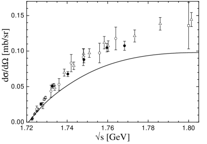
Figure 2: Differential cross section for backward $\omega$ c.m. angles. The data points are from $\bullet$: binnie , $\triangle$: keyne , $\circ$: karami , and $\Box$: danburg . The curve gives the result of a coupled-channel analysis moretocome .

It is important to notice that in the data analysis both $\mathrm{p}^{\prime}_{L}$ and $x_{L}$ are needed to fix the kinematics of the measured events. During the count rate corrections (flux normalization in dependence on $\mathrm{k}_{L}$, background subtraction via missing mass spectra), for each $\mathrm{k}_{L}$ beam setting the measured $\mathrm{p}^{\prime}_{L}$ and $x_{L}$ translate into $\sqrt{q^{2}}$ (see (II)) and can also be Lorentz transformed into their c.m. values $\mathrm{p}^{\prime}=\mathrm{p}^{\prime}({E_{\pi}}_{L},\mathrm{p}^{\prime}_{L},x_{L})$ and $x=x({E_{\pi}}_{L},\mathrm{p}^{\prime}_{L},x_{L})$. The events can now be regrouped in $\mathrm{p}^{\prime}$, $\sqrt{q^{2}}$, and $x$ intervals. Then, after having performed the integration over all $\sqrt{q^{2}}$ as in (12), the translation of a given $\mathrm{p}^{\prime}$ into $\sqrt{s}$ can only be done by assuming that the main contribution to the corrected count rates comes from around the peak of the omega spectral function $q^{2}\sim m_{\omega}^{2}$.

The main assertion of ref. hanhart99 , manifested in eqn. (H4), is that instead of (12) only a fraction of the cross section for the production of an unstable particle had been measured in binnie ; keyne ; karami . This fraction is determined by translating the experimental $\mathrm{p^{\prime}}$ binning intervals given in karami into interval bounds for the integration over the $\omega$ spectral function. Equation (H4), which is used for the cross section corrections in sibi ; titov ; hanhart01 , is identical to the third line of eqn. (II) under the assumption that $\mathrm{p^{\prime}}$ is bound to the $\mathrm{p^{\prime}}$ binning intervals. However, as pointed out above, in an experimental event ${E_{\pi}}_{L}$, $\mathrm{p}^{\prime}_{L}$, and $x_{L}$ are fixed and hence eqn. (11) has to be applied to the experimental count rate for a fixed pion momentum.

The experimental integration over the incoming pion momentum is introduced in ref. hanhart99 only in the subsequent discussion between eqns. (H9) and (H10). In the paragraph following eqn. (H16) the authors of ref. hanhart99 argue that the range of this integral is narrowed due to the $\mathrm{p^{\prime}}$ binning (as in (H4)). The $\omega$ mass is thus allowed to vary only in the interval given by the $\mathrm{p^{\prime}}$ interval ranges for a fixed pion momentum. But as shown above, fixing $\mathrm{p^{\prime}}$ only fixes the incoming pion momentum if one assumes a specific $\omega$ mass. Hence the pion momentum integration performed in the data analysis indeed translates into an $\omega$ mass integration only bounded by the pion momentum range and thus leads to eqn. (12). This relation between the neutron momentum $\mathrm{p^{\prime}}$, the pion momentum $\mathrm{k}$, and the $\omega$ mass were thus treated improperly in ref. hanhart99 .

The second correction factor extracted in ref. hanhart99 due to the neutron momentum binning of $\Delta\mathrm{p}^{\prime}=10$ MeV is nothing but the result of averaging the third line of eqn. (II) over the neutron c.m. momentum: $(\Delta\mathrm{p}^{\prime})^{-1}\int_{\mathrm{p}^{\prime}-\Delta\mathrm{p}^{\prime}}^{\mathrm{p}^{\prime}+\Delta\mathrm{p}^{\prime}}{\tilde{\mathrm{p}}}^{2}\mathrm{d}\tilde{\mathrm{p}}={\mathrm{p}^{\prime}}^{2}+(\Delta\mathrm{p}^{\prime})^{2}/12$ (cf. (H10)). This differs at most (“worst” case: $\mathrm{p}^{\prime}=30$ MeV) by 1 percent from ${\mathrm{p}^{\prime}}^{2}$ and is therefore negligible.

Furthermore, it is obvious from figs. 2 and 3

Figure 3: Differential cross section for forward $\omega$ c.m. angles. For the notations see fig. 2.

that the differential $\omega N$ data from all three references binnie ; keyne ; karami are completely in line with each other and also with ref. danburg . The same holds true for the total cross sections of ref. karami in comparison with other experiments, see fig. 4.

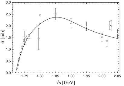
Figure 4: $\pi N\rightarrow\omega N$ total cross section. Data are from $\circ$: karami , $\bigtriangledown$: landolt , $\Box$: danburg . The curve gives the result of a coupled-channel analysis moretocome .

There is, therefore, no reason to hypothesize – as in hanhart01 – that the formalism developed in binnie could have been used incorrectly in keyne and karami .

In this context we stress one more point. Very close to threshold, the two-body cross section $\pi^{-}p\rightarrow\omega n$ extracted from experimental count rates could be influenced by the strong $\pi N$ interaction for slow pions stemming from $\omega\rightarrow 3\pi$. However, this point was checked in ref. keyne by also looking at $\omega\rightarrow\pi^{0}\gamma$; they did not find any deviations between the two ways of extraction.

III Summary and Conclusion

We have shown that the extraction method presented in binnie and also used in keyne ; karami is indeed correct. There is no reason to doubt the correctness of the data presented in these references; they are in line with each other and also with other experimental data. The reanalysis of the $\omega N$-production data in ref. hanhart99 , on which the theoretical descriptions of refs. sibi ; titov are based, as well as the speculations in ref. hanhart01 thus lack any basis. In ref. moretocome we show how the $\pi^{-}p\rightarrow\omega n$ cross section at threshold can be understood in a coupled-channel analysis.

References

• (1) D.M. Binnie et al., Phys. Rev. D 8, 2789 (1973).
• (2) J. Keyne, D.M. Binnie, J. Carr, N.C. Debenham, A. Duane, D.A. Garbutt, W.G. Jones, I. Siotis, and J.G. McEwen, Phys. Rev. D 14, 28 (1976).
• (3) H. Karami, J. Carr, N.C. Debenham, D.A. Garbutt, W.G. Jones, D.M. Binnie, J. Keyne, P. Moissidis, H.N. Sarma, and I. Siotis, Nucl. Phys. B154, 503 (1979).
• (4) F. Klingl, Ph.D. thesis, University of Munich, Hieronymus, Munich 1998.
• (5) M. Post and U. Mosel, Nucl. Phys. A688, 808 (2001).
• (6) M. Lutz, G. Wolf, and B. Friman, Nucl. Phys. A661, 526c (1999) and Proceedings of the International Workshop XXVIII on Gross Properties of Nuclei and Nuclear Excitations: Hirschegg, Austria, 16-22 Jan. 2000, Editors: M. Buballa, B.-J. Schaefer, W. NΓΆrenberg, J. Wambach, GSI; e-Print ArXive: nucl-th/0003012.
• (7) C. Hanhart and A. Kudryavtsev, Eur. Phys. J. A 6, 325 (1999).
• (8) A. Sibirtsev and A. Cassing, Eur. Phys. J. A 7, 407 (2000).
• (9) A.I. Titov, B. KΓ€mpfer, and B.L. Reznik, e-Print ArXive: nucl-th/0102032.
• (10) C. Hanhart, A. Sibirtsev, and J. Speth, e-Print ArXive: nucl-th/0107245.
• (11) H. HΓΆhler, Landolt-BΓΆrnstein, Vol. 9, Springer, Berlin 1983.
• (12) We thank C. Hanhart for pointing out this second possibility to us.
• (13) M.M. Pavan, R.A. Arndt, I.I. Strakovsky, and R.L. Workman, Phys. Scripta T87 62 (2000), e-Print ArXive nucl-th/9807087, R.A. Arndt, I.I. Strakovsky, R.L. Workman, and M.M. Pavan, Phys. Rev. C 52, 2120 (1995), updates available via: http://gwdac.phys.gwu.edu/.
• (14) D.M. Manley, R.A. Arndt, Y. Goradia, and V.L. Teplitz, Phys. Rev. D 30, 904 (1984).
• (15) G. Penner and U. Mosel, submitted to Phys. Rev. C, e-Print ArXive: nucl-th/0111023.
• (16) B. Friman, Proceedings of the APCTP-Workshop on Astro-Hadron Physics, Seoul, Korea, October 1997, e-Print ArXive: nucl-th/9801053.
• (17) F. Klingl, T. Waas, and W. Weise, Nucl. Phys. A650, 299 (1999).
• (18) C. Itzykson and J.-B. Zuber, Quantum Field Theory, McGraw-Hill, New York 1980.
• (19) J.S. Danburg, M.A. Abolins, O.I. Dahl, D.W. Davies, P.L. Hoch, J. Kirz, D.H. Miller, and R.K. Rader, Phys. Rev. D 2, 2564 (1970).