$\pi N\rightarrow\omega N$ in a coupled-channel approach

Abstract

We describe the $\pi N\rightarrow\omega N$ cross section from threshold to a center of mass energy of $2$ GeV in a unitary coupled-channel model and analyze it in terms of rescattering and resonance excitations. The amplitude is mainly composed of $D_{13}$, $P_{13}$, and $P_{11}$ contributions, where the $D_{13}$ dominates over the complete considered energy range. We also outline the generalization of the standard partial-wave formalism necessary for the decomposition of the $\omega N$ final state.

I Introduction

The reliable extraction of nucleon resonance properties from experiments where the nucleon is excited via either hadronic or electromagnetic probes is one of the major issues of hadron physics. The goal is to be finally able to compare the extracted masses and partial decay widths to predictions from lattice QCD (e.g., flee ) and/or quark models (e.g., capstick ; riska ).

With this aim in mind we developed in feusti a unitary coupled-channel effective Lagrangian model that already incorporated the final states $\gamma N$, $\pi N$, $2\pi N$, $\eta N$, and $K\Lambda$ and was used for a simultaneous analysis of all avaible experimental data on photon- and pion-induced reactions on the nucleon.

In an extension of the model to higher c.m. energies, i.e., up to center-of-mass energies of $\sqrt{s}=2$ GeV for the investigation of higher and so-called hidden nucleon resonances, the consideration of other final states becomes unavoidable and hence the model is extended to also include $\omega N$ and $K\Sigma$. As can be seen from Fig. 1

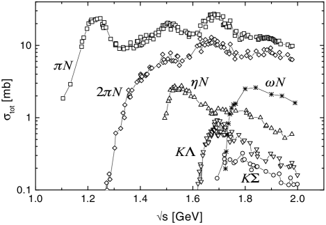
Figure 1: Total cross sections for the reactions $\pi^{-}p\rightarrow X$ with $X$ as given in the figure. All data are from ref. landolt ; the lines are to guide the eye.

for $\sqrt{s}>1.7$ GeV it is mandatory to take into account the $\omega N$ state in a unitary model. Furthermore, $\omega$ production on the nucleon represents a possibility to project out $I=\frac{1}{2}$ resonances in the reaction mechanism. However, the $\omega N$ channel resisted up to now a theoretical description in line with experiment. Especially the inclusion of nucleon Born contributions klingl overestimated the data at energies above $1.77$ GeV and only either the neglect of these diagrams post ; friman or very soft form factors titov led to a rough description of the experimental data. However, none of these models included rescattering effects or a detailed partial-wave analysis of interference effects. As recently pointed out nstar2001 both lead to strong modifications of the observed cross section; see also Fig. 2.

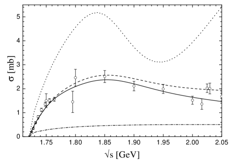
Figure 2: $\pi^{-}p\rightarrow\omega n$ total cross section. Solid line: full calculation. Dashed line: calculation with $g_{NN\omega}=7.98$, $\kappa_{NN\omega}=-0.12$. Dotted line: no rescattering. Dash-dotted line: nucleon contribution ignoring rescattering. For the data references, see Sec. IV.

The aim of this paper is to present the results of $\pi N\rightarrow\omega N$ within a coupled-channel model that simultaneously describes all pion induced data for $\pi N$, $2\pi N$, $\eta N$, $K\Lambda$, $K\Sigma$, and $\omega N$. Hence this analysis differs from all other investigations of $\pi N\rightarrow\omega N$ in two respects: First, a larger energy region is considered, which also means there are more restrictions from experiment, and second, the reaction process is influenced by all other channels and vice versa. This leads to strong constraints in the choice of $\omega N$ contributions and it is therefore possible to extract them more reliably.

We start with a short review of the model of ref. feusti in Sec. II, where we also present the way the $\omega N$ final state is included. As a result of the $\omega$ intrinsic spin the inclusion of this final state requires an extension of the standard partial-wave decomposition (PWD) method developed for $\pi N/\gamma N\rightarrow\pi N$ and $\gamma N\rightarrow\gamma N$ (see, e.g., feusti ). Such an extension is provided in Sec. III. In Sec. IV our calculations are compared to the available experimental data and we conclude with a summary.

II Model

The scattering equation that needs to be solved is the Bethe-Salpeter (BS) equation for the scattering amplitude:

$$M(p^{\prime},p;\sqrt{s}) = V(p^{\prime},p;\sqrt{s})$$ (1)

$$+\int\frac{\mathrm{d}^{4}q}{(2\pi)^{4}}V(p^{\prime},q;\sqrt{s})$$

$$\;\;\;\;\times G_{BS}(q;\sqrt{s})M(q,p;\sqrt{s})\;.$$

Here, $p$ ($k$) and $p^{\prime}$ ($k^{\prime}$) are the incoming and outgoing baryon (meson) four-momenta. After splitting up the two-particle BS propagator $G_{BS}$ into its real and imaginary parts, one can introduce the $K$-matrix via (in a schematical notation) $K=V+\int V\mathrm{Re}G_{BS}M$. Then $M$ is given by $M=K+i\int M\mathrm{Im}G_{BS}K$. Since the imaginary part of $G_{BS}$ just contains its on-shell part, the reaction matrix $T$, defined via the scattering matrix $S=1+2iT$, can now be calculated from $K$ after a PWD in $J$, $P$, and $I$ via matrix inversion:

$$T(p^{\prime},p;\sqrt{s})=\frac{K(p^{\prime},p;\sqrt{s})}{1-iK(p^{\prime},p;\sqrt{s})}.$$ (2)

Hence unitarity is fulfilled as long as $K$ is Hermitian. For simplicity we apply the so-called $K$-matrix Born approximation, which means that we neglect the real part of $G_{BS}$ and thus $K$ reduces to $K=V$. The validity of this approximation was tested by Pearce and Jennings pearce . By fitting the $\pi N$ elastic phase shifts also using other intermediate propagators for $G_{BS}$ these authors found no significant differences in the extracted parameters.

The potential $V$ is built up by a sum of $s$-, $u$-, and $t$-channel Feynman diagrams by means of effective Lagrangians which can be found in feusti . The background (nonresonant) contributions to the amplitudes are not added “by hand”, but are consistently created by the $u$- and $t$-channel diagrams. Thus the number of parameters is greatly reduced. This holds true for the reaction $\pi^{-}p\rightarrow\omega N$ in the same way, where we also allowed for the nucleon Born diagrams and a $\rho$ exchange in the $t$ channel. In our model the following 14 resonances are included: $P_{33}(1232)$, $P_{11}(1440)$, $D_{13}(1520)$, $S_{11}(1535)$, $P_{33}(1600)$, $S_{31}(1620)$, $S_{11}(1650)$, $D_{33}(1700)$, $P_{11}(1710)$, $P_{13}(1720)$, $P_{31}(1750)$, $P_{13}(1900)$, $P_{33}(1920)$, and a $D_{13}(1950)$ (as in feusti ; bennhold ) which is listed as $D_{13}(2080)$ by the Particle Data Group pdg .

The resonance $\omega N$ Lagrangians have been chosen as a compromise of an extension of the usual $RN\gamma$ transitions feusti [for vector meson dominance (VMD) reasons] and the compatibility with other $RN$ vector meson couplings used in the literature riska ; titov ; postrho ; the latter point is discussed in Sec. IV. For the spin-$\frac{1}{2}$ resonances we apply the same $\omega N$ Lagrangian as for the nucleon ($\omega N\rightarrow R$):

$${\mathcal{L}}=-\bar{R}\left(\begin{array}[]{c}1\\ -i\gamma_{5}\end{array}\right)\left(g_{1}\gamma_{\mu}-\frac{g_{2}}{2m_{N}}\sigma_{\mu\nu}\partial^{\nu}_{\omega}\right)N\omega^{\mu}\;,$$ (3)

where the first coupling is the same one as in riska ; titov since the $\omega$ is polarized such that $k^{\prime}_{\mu}\omega^{\mu}=0$. For the spin-$\frac{3}{2}$ resonances we use

$${\mathcal{L}} = -\bar{R}^{\mu}\left(\begin{array}[]{c}i\gamma_{5}\\ 1\end{array}\right)\left(\frac{g_{1}}{2m_{N}}\gamma^{\alpha}+i\frac{g_{2}}{4m_{N}^{2}}\partial^{\alpha}_{N}+i\frac{g_{3}}{4m_{N}^{2}}\partial^{\alpha}_{\omega}\right)$$ (7)

$$\times\left(\partial^{\omega}_{\alpha}g_{\mu\nu}-\partial^{\omega}_{\mu}g_{\alpha\nu}\right)N\omega^{\nu}\;.$$

In both equations the upper operator ($1$ or $i\gamma_{5}$) corresponds to a positive- and the lower one to a negative-parity resonance. For positive-parity spin-$\frac{3}{2}$ resonances the first coupling is also the same as used in riska ; titov ; for negative parity a combination of our first two couplings corresponds on shell to theirs. The above couplings have also been applied in postrho in calculations of the $\rho$ spectral function.

Each vertex is multiplied with a cutoff function as in feusti :

$$F(q^{2})=\frac{\Lambda_{q}^{4}}{\Lambda_{q}^{4}+(q^{2}-m_{q}^{2})^{2}}\;,$$ (8)

where $m_{q}$ ($q^{2}$) denotes the mass (four-momentum squared) of the off-shell particle. To reduce the number of parameters the cutoff value $\Lambda_{q}$ is chosen to be identical for all final states. We only distinguish between the nucleon cutoff ($\Lambda_{N}$), the spin-$\frac{1}{2}$ ($\Lambda_{\frac{1}{2}}$) and spin-$\frac{3}{2}$ ($\Lambda_{\frac{3}{2}}$) resonance cutoffs, and the $t$-channel cutoff ($\Lambda_{t}$), i.e., only four different cutoff parameters.

From the couplings in Eqs. (3) and (7) the helicity decay amplitudes of the resonances to $\omega N$ can be deduced:

$$A^{\omega N}_{\frac{1}{2}} = \mp\frac{\sqrt{E_{N}\mp m_{N}}}{\sqrt{m_{N}}}\left(g_{1}+g_{2}\frac{m_{N}\pm m_{R}}{2m_{N}}\right)\;,$$ (9)

$$A^{\omega N}_{0} = \mp\frac{\sqrt{E_{N}\mp m_{N}}}{m_{\omega}\sqrt{2m_{N}}}\left(g_{1}(m_{N}\pm m_{R})+g_{2}\frac{m_{\omega}^{2}}{2m_{N}}\right)\;,$$

for spin-$\frac{1}{2}$ and

$$A^{\omega N}_{\frac{3}{2}} = -\frac{\sqrt{E_{N}\mp m_{N}}}{\sqrt{2m_{N}}}\frac{1}{2m_{N}}\left(g_{3}\frac{m_{\omega}^{2}}{2m_{N}}-g_{1}(m_{N}\pm m_{R})+g_{2}\frac{m_{R}^{2}-m_{N}^{2}-m_{\omega}^{2}}{4m_{N}}\right)\;,$$

$$A^{\omega N}_{\frac{1}{2}} = \pm\frac{\sqrt{E_{N}\mp m_{N}}}{\sqrt{6m_{N}}}\frac{1}{2m_{N}}\left(g_{3}\frac{m_{\omega}^{2}}{2m_{N}}\pm g_{1}\frac{m_{N}(m_{N}\pm m_{R})-m_{\omega}^{2}}{m_{R}}+g_{2}\frac{m_{R}^{2}-m_{N}^{2}-m_{\omega}^{2}}{4m_{N}}\right)\;,$$

$$A^{\omega N}_{0} = \pm m_{\omega}\frac{\sqrt{E_{N}\mp m_{N}}}{\sqrt{3m_{N}}}\frac{1}{2m_{N}}\left(g_{1}\mp g_{2}\frac{m_{R}^{2}+m_{N}^{2}-m_{\omega}^{2}}{4m_{R}m_{N}}\mp g_{3}\frac{m_{R}^{2}-m_{N}^{2}+m_{\omega}^{2}}{4m_{R}m_{N}}\right)\;,$$ (10)

for spin-$\frac{3}{2}$ resonances. Again, the upper sign holds for positive- and the lower for negative-parity resonances. The lower indices correspond to the resonance helicities and are determined by the $\omega$ and nucleon spin $z$ components: $\frac{3}{2}$: $1+\frac{1}{2}=\frac{3}{2}$, $\frac{1}{2}$: $1-\frac{1}{2}=\frac{1}{2}$, and $0$: $0+\frac{1}{2}=\frac{1}{2}$. The resonance $\omega N$ decay widths are then given by

$$\Gamma^{\omega N}=\frac{2}{2J+1}\sum\limits_{\lambda=0}^{\lambda=+J}\Gamma^{\omega N}_{\lambda}\;,\hskip 11.38109pt\Gamma^{\omega N}_{\lambda}=\frac{\mathrm{k}^{\prime}m_{N}}{2\pi m_{R}}\left|A^{\omega N}_{\lambda}\right|^{2}$$ (11)

(upright letters denote the absolute value of the corresponding three- momentum). As a result of the limited amount of experimental data (we included 114 $\omega N$ data points in the fitting procedure; cf. Sec. IV) we tried to minimize the set of parameters and only varied a subset of the $\omega N$ coupling constants. This also means that it is not possible to distinguish with certainty between the different choices of the $RN\omega$ couplings, especially for those resonances with only small contributions to $\omega N$. Only more $\omega N$ data in the higher-energy region, i.e., above $\sqrt{s}=1.77$ GeV, and the inclusion of photoproduction data in the analysis moretocome could shed more light on the situation. However, as shown in Sec. IV, the choice of couplings presented in the following allows a complete description of the angular and energy dependences of the $\omega N$ production process.

In the process of the fitting procedure we allowed for two different couplings ($g_{1}$ and $g_{2}$) to $\omega N$ for those resonances which turned out to couple strongly to this final state, i.e., $P_{11}(1710)$, $P_{13}(1720)$, $P_{13}(1900)$, and $D_{13}(1950)$, and one coupling ($g_{1}$) for the $S_{11}(1650)$. Since the usual values for the $NN\omega$ couplings (cf. Ref. feusti and references therein) stem from different kinematical regimes than the one examined here, we also allowed these two values to be varied during the fitting procedure. But at the same time, the cutoff value in the vertex form factor is not allowed to vary freely; instead, the same value is used for all final states (see Sec. IV). It is also important to notice that as a result of the coupled-channel calculation, there are also constraints from all other channels that are compared to experimental data, leading to large restrictions in the freedom of chosing the $\omega N$ contributions.

III $\omega$ Production

Since the orbital angular momentum $\ell$ is not conserved in, e.g., $\pi N\rightarrow\omega N$, the standard PWD becomes inconvenient for many of the channels that have to be included. Hence we use here a generalization of the standard PWD method which represents a tool to analyze any meson- and photon-baryon reaction on an equal, uniform footing.

We start with the decomposition of the two-particle c.m. momentum states ($\mbox{\boldmath$p\!\!$ \unboldmath}=-\mbox{\boldmath$k\!\!$ \unboldmath}$, $\mathrm{p}=|\mbox{\boldmath$p\!\!$ \unboldmath}|$) into states with total angular momentum $J$ and $J_{z}=M$ jacobwick :

$$|\mathrm{p}JM,\lambda_{k}\lambda_{p}\rangle=N_{J}\int e^{i(M-\lambda)\varphi}d^{J}_{M\lambda}(\vartheta)|\mathrm{p}\vartheta\varphi,\lambda_{k}\lambda_{p}\rangle\mbox{d}\Omega,$$

where $\lambda_{k}$ ($\lambda_{p}$) is the meson (baryon) helicity and the $d^{J}_{M\lambda}(\vartheta)$ are Wigner functions. The normalization $N_{J}$ is given by $\sqrt{(2J+1)/(4\pi)}$ and $\lambda=\lambda_{k}-\lambda_{p}$. For the incoming c.m. state ($\vartheta_{0}=\varphi_{0}=0$ $\Rightarrow$ $\ell=0$) one gets $\langle JM,\lambda_{k}\lambda_{p}|\vartheta_{0}\varphi_{0},\lambda_{k}\lambda_{p}\rangle\sim\delta_{M\lambda}$, and one can drop the index $M$. By using the parity property jacobwick $\hat{P}|J,\lambda\rangle=\eta_{k}\eta_{p}(-1)^{J-s_{k}-s_{p}}|J,-\lambda\rangle$, where $\eta_{k}$ and $\eta_{p}$ ($s_{k}$ and $s_{p}$) are the intrinsic parities (spins) of the two particles, the construction of normalized states with parity $(-1)^{J\pm\frac{1}{2}}$ is straightforward:

$$|J,\lambda;\pm\rangle \equiv \frac{1}{\sqrt{2}}\left(|J,+\lambda\rangle\pm\eta|J,-\lambda\rangle\right)$$

$$\Rightarrow\hat{P}|J,\lambda;\pm\rangle = (-1)^{J\pm\frac{1}{2}}|J,\lambda;\pm\rangle,$$ (12)

where we have defined

$$\eta\equiv\eta_{k}\eta_{p}(-1)^{s_{k}+s_{p}+\frac{1}{2}}\;.$$

They can be used to project out helicity amplitudes with parity $(-1)^{J\pm\frac{1}{2}}$:

$${\mathcal{T}}^{J\pm}_{\lambda^{\prime}\lambda}\equiv\langle J,\lambda^{\prime};\pm|T|J,\lambda;\pm\rangle={\mathcal{T}}^{J}_{\lambda^{\prime}\lambda}\pm\eta{\mathcal{T}}^{J}_{\lambda^{\prime}-\lambda}\;,$$ (13)

with

$${\mathcal{T}}^{J}_{\lambda^{\prime}\lambda}(\sqrt{s}) \equiv \langle\lambda^{\prime}|T^{J}(\sqrt{s})|\lambda\rangle$$

$$= 2\pi\int\mathrm{d}(\cos\vartheta)d^{J}_{\lambda\lambda^{\prime}}(\vartheta)\langle\vartheta,\varphi=0,\lambda^{\prime}|T|00,\lambda\rangle\;.$$

In eqn. (13) we have used, that for parity conserving interactions $T=\hat{P}^{-1}T\hat{P}$:

$$\langle J,-\lambda^{\prime}|T|J,-\lambda\rangle=\eta(\eta^{\prime})^{-1}\langle J,\lambda^{\prime}|T|J,\lambda\rangle\;.$$ (14)

The helicity amplitudes ${\mathcal{T}}^{J\pm}_{\lambda^{\prime}\lambda}$ have definite, identical $J$ and definite, but opposite $P$. As is quite obvious this method is valid for any meson-baryon final state combination, even such cases as, e.g., $\omega N\rightarrow\pi\Delta$. In the case of $\pi N\rightarrow\pi N$ the ${\mathcal{T}}^{J\pm}_{\lambda^{\prime}\lambda}$ coincide with the conventional partial-wave amplitudes: ${\mathcal{T}}^{J\pm}_{\frac{1}{2}\frac{1}{2}}\equiv{\mathcal{T}}_{\ell\pm}$.

IV Comparison with Experiment

For the fitting procedure we modified the data set used in Ref. feusti in the following way.

For $\pi N\rightarrow\pi N$ we used the updated single-energy partial-wave analysis SM00 SM00 . For $2\pi N$, $\eta N$, and $K\Lambda$ we continue to use the same database as in feusti ; however, for $\eta N$ the data from morrison and for $K\Lambda$ the data from lambdaexp were added. For $K\Sigma$ production we used the total cross section, angle-differential cross section, and polarization data from haba and from the references to be found in landolt .

Furthermore, we have included all the $\pi N\rightarrow\omega N$ data in the literature binnie ; keyne ; karami ; danburg . At this point we wish to stress that we do not follow the authors of Refs. hanhart99 ; hanhart01 to “correct” the Karami karami data. The authors of hanhart99 have claimed that the method used in binnie ; keyne ; karami to extract the two-body cross section from the count rates was incorrect. However, a careful reading of Ref. binnie reveals that the two-body cross sections were indeed correctly deduced and the peak region of the $\omega$ spectral function is well covered even at energies close to the $\omega$ production threshold. The conclusion of Ref. hanhart99 can be traced back to the incorrect reduction of the integration over the $\omega$ spectral function to the experimental averaging over the outgoing neutron c.m. momentum interval binning; a detailed discussion can be found in fightforkarami . See also the discussion about the $\pi N$ inelasticities below.

The results presented in the following are from ongoing calculations to describe the data of all channels simultaneously (cf. Table 1).

Total	$\pi N$	$2\pi N$	$\eta N$	$K\Lambda$	$K\Sigma$	$\omega N$
3.08	3.78	6.95	1.78	2.05	2.43	2.53

Table 1: $\chi^{2}$ per degree of freedom from the present calculation for $\pi N\rightarrow X$ with $X$ as given in the table.

The coupling set used for the presented results leads to an overall $\chi^{2}$ of 3.08 per degree of freedom (by comparison to a total of $2360$ data points).

As can be seen in Figs. 3 and 4

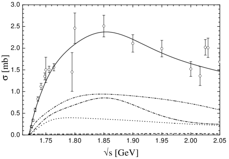
Figure 3: $\pi^{-}p\rightarrow\omega n$ total cross section. The contributions of various partial waves are given by $J^{P}=\frac{1}{2}^{-}(S_{11})$: dashed line; $\frac{1}{2}^{+}(P_{11})$: dotted line; $\frac{3}{2}^{+}(P_{13})$: dash-dotted line; $\frac{3}{2}^{-}(D_{13})$: dash-double-dotted line (in brackets the $\pi N$ notation is given). The sum of all partial waves is given by the solid line. For the data references, see text.

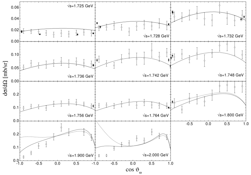
Figure 4: $\pi^{-}p\rightarrow\omega n$ differential cross section. Data are from $\bullet$: binnie ; keyne , $\circ$: karami , and $\Box$: danburg . For the data points extracted from Ref. danburg see text. At energies $\sqrt{s}\geq 1.8$ GeV also a calculation with $g_{NN\omega}=7.98$, $\kappa_{NN\omega}=-0.12$ is shown (dashed line).

our calculation is in line with all total and also with the differential $\omega N$ cross sections of Refs. binnie ; keyne ; karami . To get a handle on the angle-differential structure of the cross section for energies $\sqrt{s}\geq 1.8$ GeV we also extracted angle-differential cross sections from the corrected cosine event distributions given in Ref. danburg with the help of their total cross sections. These data points strongly constrain the nucleon $u$-channel contribution because of the decrease at backward angles; see the end of this section. Moreover, for these energies the contribution of the $\rho$ exchange contribution leads to an increasing forward peaking behavior.

The total $\omega N$ cross section (cf. Fig. 3) is dominantly composed of two partial waves contributing with approximately the same magnitude $J^{P}=\frac{3}{2}^{-}(D_{13})$ and $\frac{3}{2}^{+}(P_{13})$, and also a smaller $\frac{1}{2}^{+}(P_{11})$ contribution, while the $\frac{1}{2}^{-}(S_{11})$ partial wave is almost negligible (in brackets the $\pi N$ notation is given). The main contributions in these partial waves stem from the $D_{13}(1950)$, the $P_{13}(1720)$, the nucleon, and the $P_{11}(1710)$. The $D_{13}(1950)$ is especially interesting, since it is only listed in the PDG pdg at $2.08$ GeV, but was already found as an important contribution in $\pi N$ and $K\Lambda$ channels (cf. feusti ; bennhold ) at around $1.95$ GeV. In our calculation it turns out to be an important production mechanism as well, in particular at threshold. These findings are also contrary to the conclusions drawn in karami . Guided by their angle-differential cross sections they excluded any noticeable $J=\frac{3}{2}$ effects and deduced a production mechanism that is dominated by $J=\frac{1}{2}$ contributions. However, our coupled-channel calculation shows that their angle-differential cross sections can indeed be described by dominating $\frac{3}{2}^{-}$ and $\frac{3}{2}^{+}$ waves. Furthermore, since the data in all other channels (including $\pi N$ inelasticities and $2\pi N$ partial wave cross sections in the isospin-$\frac{1}{2}$ partial waves; see below) are also very well described in the $\omega N$ threshold region ($1.72$ GeV $<\sqrt{s}<1.76$ GeV), our partial-wave decomposition of $\pi N\rightarrow\omega N$ is on safe grounds.

As a result of the coupled-channel calculation, the opening of the $\omega N$ channel also becomes visible in the inelasticity of the $\pi N\rightarrow\pi N$ channel. In figs. 5 and 6

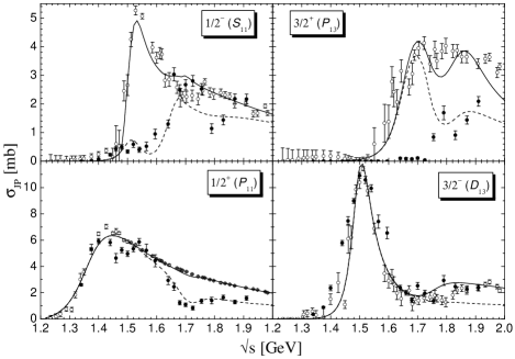
Figure 5: $\pi N\rightarrow\pi N$ inelastic ($\circ$ as extracted from SM00 SM00 , calculation: solid line) and $\pi N\rightarrow 2\pi N$ partial-wave cross sections ($\bullet$ as extracted by manley , calculation: dashed line), both for $I=\frac{1}{2}$. For the discrepancy of $\pi N\rightarrow 2\pi N$ in the $\frac{3}{2}^{+}(P_{13})$ partial wave between $1.52$ and $1.725$ GeV see text.

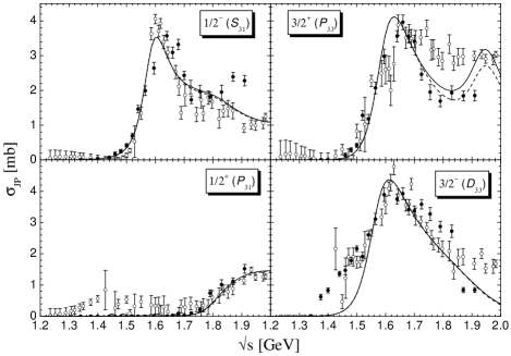
Figure 6: $\pi N\rightarrow\pi N$ inelastic ($\circ$ as extracted from SM00 SM00 , calculation: solid line) and $\pi N\rightarrow 2\pi N$ partial-wave cross sections ($\bullet$ as extracted by manley , calculation: dashed line), both for $I=\frac{3}{2}$.

the $\pi N\rightarrow\pi N$ inelastic

$$\sigma^{in}_{IJ\pm}=\frac{4\pi}{\mathrm{k}^{2}}\left(J+\frac{1}{2}\right)\left(\mathrm{Im}{\mathcal{T}}^{IJ\pm}_{\frac{1}{2}\frac{1}{2}}-\left|{\mathcal{T}}^{IJ\pm}_{\frac{1}{2}\frac{1}{2}}\right|^{2}\right)$$ (15)

and the $\pi N\rightarrow 2\pi N$ partial-wave cross sections

$$\sigma^{2\pi}_{IJ\pm}=\frac{4\pi}{\mathrm{k}^{2}}\left(J+\frac{1}{2}\right)\left|{\mathcal{T}}^{IJ\pm}_{\frac{1}{2}\frac{1}{2}}\right|^{2}$$ (16)

are plotted together with experimental data from SM00 SM00 and manley . An $IJ^{P}=\frac{1}{2}\frac{1}{2}^{-}$ or $\frac{1}{2}\frac{3}{2}^{-}$ wave contribution in the order of $\sigma_{\omega N}\geq 3$ mb for $1.72$ GeV $\leq\sqrt{s}\leq$ $1.74$ GeV as claimed in hanhart99 ; hanhart01 would also be in contradiction with inelasticities extracted from $\pi N\rightarrow\pi N$ partial waves: The $\frac{1}{2}\frac{1}{2}^{-}$ inelasticity around the $\omega N$ threshold is already saturated by the $2\pi N$ and $K\Sigma$ channels; a large $\omega N$ contribution would spoil the agreement between calculation and experiment; the $\frac{1}{2}\frac{3}{2}^{-}$ inelasticity allows only $\sigma^{\omega N}_{\frac{1}{2}\frac{3}{2}^{-}}\leq\sigma^{in}_{\frac{1}{2}\frac{3}{2}^{-}}-\sigma^{2\pi}_{\frac{1}{2}\frac{3}{2}^{-}}\approx 1$ mb in this energy region.

At this point a remark on the $IJ^{P}=\frac{1}{2}\frac{3}{2}^{+}$ inelasticity between $1.52$ and $1.725$ GeV is in order. This inelasticity grows up to $4$ mb below the $\omega N$ threshold, while the $2\pi N$ partial-wave cross section extracted by manley is still zero. At the same time all total cross sections from other open inelastic channels ($\eta N$, $K\Lambda$, and $K\Sigma$) add up to significantly less than $4$ mb. This indicates that either the extracted $2\pi N$ partial wave cross section is not correct in the $\frac{1}{2}\frac{3}{2}^{+}$ partial wave or another inelastic channel (i.e., a $3\pi N$ channel) contributes significantly to this partial wave. Note that we only observe this effect in this partial wave and are also able to describe the inelasticity and the $2\pi N$ data above the $\omega N$ threshold in the $\frac{1}{2}\frac{3}{2}^{+}$ partial wave. Therefore, we did not introduce an additional final state but effectively neglected the $\frac{1}{2}\frac{3}{2}^{+}$ $2\pi N$ data points in the energy region between $1.52$ and $1.725$ GeV.

Another coupled-channel effect shows up in the total $\pi^{-}p\rightarrow K^{0}\Lambda$ cross section. As can be seen in Fig. 7

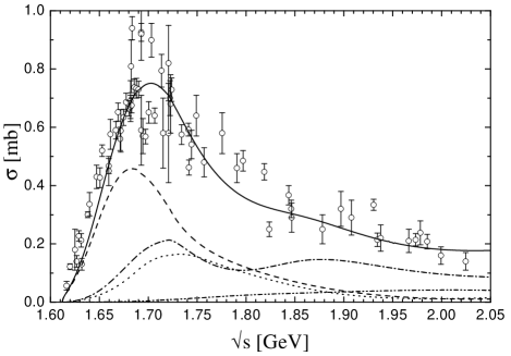
Figure 7: $\pi^{-}p\rightarrow K^{0}\Lambda$ total cross section. See Fig. 3 for the notation. For the data references, see text.

this channel exhibits a resonancelike behavior for energies $1.67$ GeV$\leq\sqrt{s}\leq 1.73$ GeV. However, this structure is also caused by the opening of two new channels, which take away the flux in the $\frac{1}{2}^{-}$ and $\frac{3}{2}^{+}$ partial waves. First, around $1.69$ GeV the $K\Sigma$ channel opens up with a strong $IJ^{P}=\frac{1}{2}\frac{1}{2}^{-}$ contribution. Second, around $1.72$ GeV $\omega N$ opens up with a small $\frac{1}{2}\frac{1}{2}^{-}$ but a strong $\frac{1}{2}\frac{3}{2}^{+}$ wave. The $\pi N\rightarrow K\Sigma$ cross sections are shown in Fig. 8.

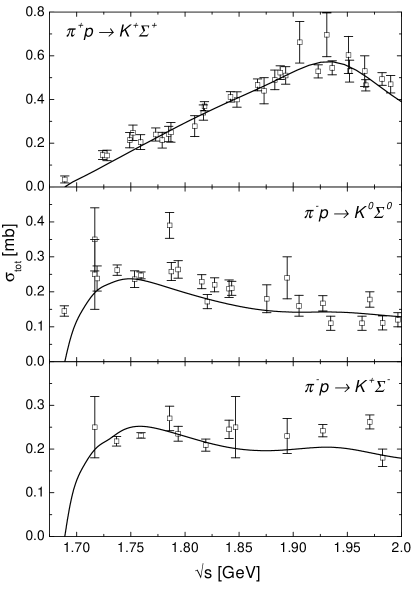
Figure 8: $\pi N\rightarrow K\Sigma$ total cross sections.

The pure $I=\frac{3}{2}$ channel $\pi^{+}p\rightarrow K^{+}\Sigma^{+}$ is strongly dominated by a $\frac{3}{2}\frac{3}{2}^{+}$ wave and also becomes visible in the $\frac{3}{2}\frac{3}{2}^{+}$ $\pi N$ inelasticity (cf. Fig. 6), while the other two channels $\pi^{-}p\rightarrow K^{0}\Sigma^{0}/K^{+}\Sigma^{-}$ show the strong $\frac{1}{2}\frac{1}{2}^{-}$ wave rise just above threshold.

As mentioned above we also allowed for the nucleon Born contributions in $\pi N\rightarrow\omega N$ usually leading to an overestimation of the total cross section at higher energies. As can be seen in Fig. 2, the inclusion of rescattering is mandatory to be able to describe the energy-dependent behavior of the total $\pi N\rightarrow\omega N$ cross section: When we apply our best parameter set to a tree level calculation — i.e., “rescattering” is only taken into account via an imaginary part in the denominator of the resonance propagators — the calculation results in the dotted line, which is far off the experimental data. This shows the importance of “off-diagonal” rescattering such as $\pi N\rightarrow\omega N\rightarrow\pi N$ or $\pi N\rightarrow K\Lambda\rightarrow\omega N$.

The values of the $NN\omega$ couplings are mainly determined by the backward angle-differential cross section at higher energies. During the fitting procedure these couplings resulted in $g_{1}=4.50$ and $\kappa=g_{2}/g_{1}=-0.70$. The total cross section exhibits almost the same behavior when we use the values from feusti ($g_{1}=7.98$ and $\kappa=-0.12$; see the dashed line in Fig. 2); however, for energies above $\sqrt{s}=1.8$ GeV the angular dependence (see the dashed line in Fig. 4) is not in line with experiment anymore. The $NN$-meson cutoff value used for all $s$- and $u$-channel diagram vertices (hence also for the $NN\omega$ vertex) resulted in $\Lambda_{N}=1.15$ GeV.

For the other background contribution in the $\omega N$ production, i.e., the $\rho$ exchange, we used the couplings $g_{\omega\rho\pi}=2.056$ (extracted from the $\omega\rightarrow\rho\pi\rightarrow\pi^{+}\pi^{-}\pi^{0}$ width), $g_{NN\rho}=5.56$, and $\kappa_{NN\rho}=1.58$ — the latter values were extracted from the fit and are the same as in calculating $\pi N$ elastic scattering.

In Table 2

$L^{\pi N}_{2I2J}$	M	$\Gamma_{tot}$	$\Gamma^{\omega N}_{0}$	$\Gamma^{\omega N}_{\frac{1}{2}}$	$\Gamma^{\omega N}_{\frac{3}{2}}$	$\Gamma^{\omega N}$	$\Gamma^{\omega N}$ of capstick
$S_{11}(1650)$	1677.5	177	-0.224a	0.0ab	–	–	–
$P_{11}(1710)$	1786.3	686	76	69	–	145	$0.0\;\scriptstyle{{+5.3}\atop{-0.0}}$
$P_{13}(1720)$	1722.5	252	0.05	0.11	1.18	0.67	$0.0\;\scriptstyle{{+1.7}\atop{-0.0}}$
$P_{13}(1900)$	1951.0	585	21	0	226	123	$20.3\scriptstyle{{+34.8}\atop{-0.0}}$
$D_{13}(1950)$	1946.0	948	162	0	289	226	$39.7\scriptstyle{{+56.3}\atop{-21.2}}$

Table 2: Masses, total, and $\omega N$ widths (see Eqn. (11)) for $I=\frac{1}{2}$ resonances coupling to $\omega N$. All values are given in MeV. For the $\omega N$ widths of ref. capstick , we also cite the upper and lower values of their extracted ranges. ^aThe couplings $g_{1}$, $g_{2}$ are given. ^bNot varied in the fit; see text.

the resonance properties of those resonances which couple to $\omega N$ are presented. In contrast to capstick ; riska ; titov we also find strong contributions from the $P_{11}(1710)$ and the $P_{13}(1720)$ resonances, where the latter one is located just above the $\omega N$ threshold of $1.721$ GeV. Our extracted $P_{11}(1710)$ width is significantly larger than the PDG pdg value of $\approx 100$ MeV, but consistent with the value of $480\pm 230$ MeV extracted by a resonance parametrization of $\pi N\rightarrow\pi N$ and $\pi N\rightarrow 2\pi N$ manley92 . The reason for these large differences is the lack of a prominent resonant behavior in the upper energy region of the $P_{11}$ $\pi N\rightarrow\pi N$ partial wave. Thus the extraction of resonance parameters is not well constrained by $\pi N\rightarrow\pi N$ alone. In our analysis the large width comes to about one-fourth from $\omega N$ and the remainder is due to $2\pi N$ ($268$ MeV), $\eta N$ ($160$ MeV), and $K\Sigma$ ($71$ MeV). In the latter two channels strong $P_{11}$ contributions are needed to describe the corresponding angle-differential cross sections and polarization observables.

We can also compare our $S_{11}(1650)$ and $P_{13}(1720)$ couplings to the one from riska ; titov if we choose to take the same width for the $P_{13}$, but only use the first coupling ($g_{1}$). While we find only a small $S_{11}$ coupling of $g_{1}=-0.22$, but a large value of $g_{1}=29.3$ for the $P_{13}$, riska ; titov found $-2.56$ and $3.17$, respectively. However, as is clear from the discussion above, a strong $P_{13}$ and a small $S_{11}$ are mandatory results of our coupled-channel analysis. For the $P_{11}(1710)$, $P_{13}(1720)$, and $D_{13}(1950)$ also a comparison to the VMD predictions of Ref. post is possible. The authors of Ref. post used different photon helicity amplitude analyses to extract ranges for the $RN\omega$ transition couplings under the assumption of strict VMD. Using their notation we find from our widths the following couplings: $P_{11}(1710)$: $6.3$ ($0$–$1.22$), $P_{13}(1720)$: $15.6$ ($0$–$5.0$), and $D_{13}(1950)$: $2.3$ ($0$–$2.6$). In brackets, their VMD ranges are given. As a result of the large uncertainties in the photon helicity amplitudes, which are the input to the calculation of post , it is impossible to draw any conclusion on the validity of strict VMD for these resonances.

V Conclusions and Outlook

In this paper we have included the $\omega N$ final state into our coupled-channel model and have investigated whether it is possible to find a way to describe the hadronic $\omega N$ data. The results of our calculations show that for a description of the reaction $\pi^{-}p\rightarrow\omega N$ in line with experimental data a unitary, coupled-channel calculation is mandatory, and the resulting amplitude is mainly composed of $IJ^{P}=\frac{1}{2}\frac{3}{2}^{-}$ ($D_{13}$), $\frac{1}{2}\frac{3}{2}^{+}$ ($P_{13}$), and $\frac{1}{2}\frac{1}{2}^{+}$ ($P_{11}$) contributions, where the $\frac{1}{2}\frac{3}{2}^{-}$ dominates over the complete considered energy range.

The next step in our investigation of nucleon resonance properties within our coupled-channel $K$-matrix model will naturally be the inclusion of photon induced data to further pin down the extracted widths and masses. The results of this study and also more details about the calculation presented here will be published soon moretocome .

Furthermore, since the partial-wave formalism is now settled, the inclusion of additional final states, in particular for a more sophisticated description of the $2\pi N$ final state, as $\rho N$ or $\pi\Delta$ is rather straightforward. Also, by the inclusion of several, e.g., $\rho N$ final states with different masses $m_{\rho}$ the width of the $\rho$ meson (and similarly for the $\Delta$) can also be taken into account. Finally, investigations concerning the inclusion of spin $\frac{5}{2}$ resonances are underway.

- (1) F.X. Lee and D.B. Leinweber, Nucl. Phys. B73, 258 (1999).
- (2) S. Capstick and W. Roberts, Phys. Rev. D 47, 1994 (1993); 49, 4570 (1994); S. Capstick and N. Isgur, ibid. 34, 2809 (1986).
- (3) D.O. Riska and G.E. Brown, Nucl. Phys. A679, 577 (2001).
- (4) T. Feuster and U. Mosel, Phys. Rev. C 58, 457 (1998); T. Feuster and U. Mosel, ibid. 59, 460 (1999).
- (5) F. Klingl, Ph.D. thesis, University of Munich (Hieronymus, Munich, 1998).
- (6) M. Post and U. Mosel, Nucl. Phys. A688, 808 (2001).
- (7) M. Lutz, G. Wolf, and B. Friman, Nucl. Phys. A661, 526c (1999); in Proceedings of the International Workshop XXVIII on Gross Properties of Nuclei and Nuclear Excitations, Hirschegg, Austria, 2000, edited by M. Buballa, B.-J. Schaefer, W. Nörenberg, J. Wambach (Gesellschaft für Schwerionenphysik (GSI), Darmstadt, 2000), nucl-th/0003012.
- (8) A.I. Titov, B. Kämpfer, and B.L. Reznik, nucl-th/0102032.
- (9) C. Hanhart and A. Kudryavtsev, Eur. Phys. J. A 6, 325 (1999).
- (10) Landolt-Börnstein, Total Cross-Sections for Reactions of High-Energy Particles, edited by H. Schopper, New Series, Group I, Vol. 12a, Pt. I (Springer, Berlin, 1988).
- (11) G. Penner and U. Mosel, in Proceedings of the Workshop on The Physics of Excited Nucleons, NStar 2001, edited by D. Drechsel and L. Tiator (World Scientific, Singapore, 2001).
- (12) B.C. Pearce and B.K. Jennings, Nucl. Phys. A528, 655 (1991).
- (13) T. Mart and C. Bennhold, Phys. Rev. C 61, 012201(R) (1999).
- (14) D.E. Groom et al., Eur. Phys. J. C 15, 1 (2000).
- (15) M. Post, S. Leupold, and U. Mosel, Nucl. Phys. A689, 753 (2001).
- (16) G. Penner and U. Mosel, in preparation.
- (17) M. Jacob and G.C. Wick, Ann. Phys. (N.Y.) 7, 404 (1959).
- (18) M.M. Pavan, R.A. Arndt, I.I. Strakovsky, and R.L. Workman, Phys. Scr. T87, 62 (2000); nucl-th/9807087, R.A. Arndt, I.I. Strakovsky, R.L. Workman, and M.M. Pavan, Phys. Rev. C 52, 2120 (1995), updates available via: http://gwdac.phys.gwu.edu/.
- (19) T.W. Morrison, Ph.D. thesis, The George Washington University, 1999.
- (20) O.I. Dahl, L.M. Hardy, R.I. Hess, J. Kirz, D.H. Miller, and J.A. Schwartz, Phys. Rev. 163, 1430 (1967); O. Goussu, M. Sen , B. Ghidini, S. Mongelli, A. Romano, P. Waloschek, and V. Alles-Borelli, Nuovo Cimento A 42, 607 (1966).
- (21) J. Haba, T. Homma, H. Kawai, M. Kobayashi, K. Miyake, T.S. Nakamura, N. Sasao, and Y. Sugimoto, Nucl. Phys. B299, 627 (1988); B308, 948(E) (1999).
- (22) D.M. Binnie et al., Phys. Rev. D 8, 2789 (1973).
- (23) J. Keyne, D.M. Binnie, J. Carr, N.C. Debenham, A. Duane, D.A. Garbutt, W.G. Jones, I. Siotis, and J.G. McEwen, Phys. Rev. D 14, 28 (1976).
- (24) H. Karami, J. Carr, N.C. Debenham, D.A. Garbutt, W.G. Jones, D.M. Binnie, J. Keyne, P. Moissidis, H.N. Sarma, and I. Siotis, Nucl. Phys. B154, 503 (1979).
- (25) J.S. Danburg, M.A. Abolins, O.I. Dahl, D.W. Davies, P.L. Hoch, J. Kirz, D.H. Miller, and R.K. Rader, Phys. Rev. D 2, 2564 (1970).
- (26) C. Hanhart, A. Sibirtsev, and J. Speth, hep-ph/0107245.
- (27) G. Penner and U. Mosel, Eur. Phys. J. A (submitted), nucl-th/0111024.
- (28) D.M. Manley, R.A. Arndt, Y. Goradia, and V.L. Teplitz, Phys. Rev. D 30, 904 (1984).
- (29) D.M. Manley and E.M. Saleski, Phys. Rev. D 45, 4002 (1992).