Nuclear Ground State Observables
and QCD Scaling in a Refined
Relativistic Point Coupling Model

Abstract

We present results obtained in the calculation of nuclear ground state properties in relativistic Hartree approximation using a Lagrangian whose QCD-scaled coupling constants are all natural (dimensionless and of order 1). Our model consists of four-, six-, and eight-fermion point couplings (contact interactions) together with derivative terms representing, respectively, two-, three-, and four-body forces and the finite ranges of the corresponding mesonic interactions. The coupling constants have been determined in a self-consistent procedure that solves the model equations for representative nuclei simultaneously in a generalized nonlinear least-squares adjustment algorithm. The extracted coupling constants allow us to predict ground state properties of a much larger set of even-even nuclei to good accuracy. The fact that the extracted coupling constants are all natural leads to the conclusion that QCD scaling and chiral symmetry apply to finite nuclei.

I INTRODUCTION

Relativistic mean field (RMF) models are quite successful in describing ground state properties of finite nuclei and nuclear matter properties. They describe the nucleus as a system of Dirac nucleons that interact in a relativistic covariant manner via mean meson fields [1, 2, 3, 4, 5, 6, 7, 8, 9] or via mean nucleon fields [10, 11] whose explicit forms sometimes derive solely from the meson field approaches [12]. The meson fields are of finite range (FR) due to meson exchange whereas the nucleon fields are of zero range (contact interactions or point couplings PC) together with derivative terms that simulate the finite range meson exchanges. There are a number of attractive features in the RMF-FR and RMF-PC approaches. These include the facts that the combined meson and/or nucleon fields account for the effective central potentials that are used in Schrödinger approaches and that the physically correct spin-orbit potential occurs naturally with magnitudes comparable to the (empirical) ad hoc spin-orbit interactions required in Schrödinger approaches. Equally attractive is the fact that for relatively few parameters $(\simeq\>10)$ a vast amount of information is obtained: the Dirac single-particle wave functions and corresponding energy eigenvalues, the ground state mass, the baryon and charge densities together with their moments, and the properties of saturated nuclear matter. Furthermore, these quantities are obtained simultaneously in the same self-consistent relativistic Hartree (or Hartree-Fock) calculation.

In this work we use mean nucleon fields constructed with contact interactions (point couplings) to represent the system of interacting Dirac nucleons. We choose this approach for the following reasons: (a) possible physical constraints introduced by explicit use of the Klein-Gordon approximation to describe mean meson fields, in particular that of the (fictitious) sigma meson, are avoided and instead the effects of the various incompletely understood and higher order processes are assumed to be lumped into appropriate coupling constants and terms of the Lagrangian, as explained in Ref. [10], (b) the use of point couplings allows not only (standard) relativistic Hartree calculations to be performed, but also relativistic Hartree-Fock calculations [13, 14] by use of Fierz relations (up to fourth order [15]), and (c) the use of point couplings, because of their success in the Nambu-Jona-Lasino model for the low-momentum domain of QCD [16], is perhaps the best way to test for naturalness of the coupling constants in the seminal Weinberg expansion [17] highlighting the role of power counting and chiral symmetry in weakening N-body forces. That is, two-nucleon forces are stronger than three-nucleon forces, which are stronger than four-nucleon forces, …, resulting in a sequence making nuclear physics tractable. If the dimensionless coupling constants of the corresponding Lagrangian are of order 1 (natural) then QCD scaling and chiral symmetry apply to finite nuclei. Finally, (d), the RMF-PC model allows one to investigate its relationship to nonrelativistic point-coupling approaches like the Skyrme-Hartree-Fock (SHF) approach and the RMF-FR approach to contrast the importance and roles of the different features these models have, as well as to obtain new insights.

Concerning point (c), the aim of this paper is to determine whether QCD scaling and chiral symmetry apply to finite nuclei and, by their application, to construct a state-of-the-art parameterization of the relativistic mean-field point-coupling Lagrangian. In the following we will use the term RMF model for both the version having finite range due to meson exchange, which we call RMF-FR, and the point-coupling (contact interaction) version that we denote by RMF-PC.

Concerning point (d), it is important to note here that one can also view RMF-PC as an approach that lies in between the RMF-FR approach and the nonrelativistic Skyrme-Hartree-Fock (SHF) approach which is also a well-developed self-consistent mean-field model that performs very well (for a review see [18]). Whereas SHF is based upon density-dependent contact interactions with extensions to gradient terms, kinetic terms, and the spin-orbit interaction, RMF-FR is based upon a coupled field theory of Dirac nucleons and effective meson fields treated at the mean-field level, where density dependence is modeled by nonlinear meson self couplings and the role of gradient terms is taken over by the finite ranges of the mesons. The kinetic and spin-orbit terms are automatically carried in both RMF models [5]. Thus, a comparison of RMF-PC and SHF addresses the differences between in-medium Dirac and Schrödinger nucleons, that is, in kinetic and spin-orbit components, whereas a comparison of RMF-PC and RMF-FR addresses the absence vs. presence of finite range and the different treatments of density dependence. Herein we will perform these comparisons using precisely the same fitting strategy as in recent SHF and RMF-FR adjustments [19, 4, 20] except that here we will in addition be guided by considerations of QCD scaling and chiral symmetry, that is, naturalness.

We regard the present work with contact interactions as a refined relativistic point coupling model in comparison to our earlier work [10, 11, 21, 22] for the following three reasons. First, initial work in determining coupling constants in RMF-PC approaches [10, 12] found a high correlation among the ground state observables used to determine them, particularly the total binding energy and the root-mean-square charge radius. Given this fact and the presence of quadratic, cubic, and quartic terms in the various densities appearing in the Lagrangian (representing two-, three-, and four-body interactions) results in very delicate cancellations among the corresponding many-body forces. This means that determination of the coupling constants using a nonlinear least-squares adjustment algorithm with respect to the corresponding measured ground-state observables is fraught with difficulty because the coupling constants are generally underdetermined. Consequently, the search for the minimum in the chi-squared hypersurface results in the location of many local minima from which erroneous conclusions can be drawn. Herein we address this problem more completely by applying two different nonlinear least-squares adjustment algorithms and, finally, developing a combined adjustment algorithm that is used to determine our present results. Second, in our initial work we considered only spherical even-even closed-shell nuclei or closed-subshell nuclei in both proton number Z and neutron number N because, due to explicit omission of the pairing interaction, we allowed only orbital occupation probabilities of 0 or 1. Here, we introduce orbital occupation probabilities for both protons and neutrons through a standard BCS approach in which the proton and neutron pairing strengths are simultaneously determined with the coupling constants in the adjustment algorithm. Third, most of our earlier work addressed the question of naturalness after the fact, that is, without consideration of the complete set of 10 possible Lorentz invariants that may occur (scalar, vector, pseudoscalar, axial vector, tensor, and the same coupled to isospin $\vec{\tau}$) and without consideration of the QCD mass-scale ordering of the terms of the Lagrangian. The former consideration is neccessary to properly pursue the question of naturalness while the latter consideration leads to, among other things, classification of the (allowed) terms of the Lagrangian according to their relative strengths, which, of course, assists in its construction in the first place. We address, and remain cognizant, of both of these considerations in the various approaches presented here.

The paper is structured as follows. The Lagrangian of our relativistic point coupling model, together with its variants, is given in Sec. II. Included are the corresponding relativistic Hartree equations, expressions for the various densities and potentials appearing, and expressions for the calculated observables that are to be used in determining the coupling constants of the Lagrangian. The approximations that we invoke are also stated here. In Sec. III we describe the determination of the coupling constants using four different least-squares adjustment algorithms with respect to well-measured ground state observables and the external constraint of always obtaining reasonable calculated values of the properties of saturated nuclear matter. A relatively new approach to the $\chi^{2}$ minimization has been developed and we explain how and why. Our results are given in Sec. IV. First, we present comparisons of calculation and experiment for nuclei whose measured observables were used to determine the coupling constants. Second, we present comparisons of predicted and measured observables for nuclei not used in determining the coupling constants. Third, we compare our results to those of other RMF approaches. Then we give our final nuclear matter predictions and we mention initial results obtained in calculating fission potential energy surfaces and properties of superheavy nuclei. We address the role of QCD scaling and chiral symmetry in Sec. V where we test our final sets of coupling constants for naturalness and present the corresponding evidence obtained that QCD and chiral symmetry apply to finite nuclei. Our conclusions and intentions for future work are given in Sec VI.

II THE MODEL

A The Lagrangian

The elementary building blocks of the point-coupling vertices are two-fermion terms of the general type

$$({\bar{\psi}}{\cal O}_{\tau}\Gamma{\psi})\quad,\quad{\cal O}_{\tau}\in\{{1},\tau_{i}\}\quad,\quad\Gamma\in\{1,\gamma_{\mu},\gamma_{5},\gamma_{5}\gamma_{\mu},\sigma_{\mu\nu}\}$$ (1)

with $\psi$ the nucleon field, $\tau_{i}$ the isospin matrices and $\Gamma$ one of the 4x4 Dirac matrices. There thus is a total of 10 such building blocks characterized by their transformation character in isospin and in spacetime.

The interactions are then obtained as products of such expressions to a given order. The products are coupled, of course, to a total isoscalar-scalar term. By “order” we mean the number of such terms in a product, so that a second-order term corresponds to a four-fermion coupling, and so on. In second order only the ten elementary currents squared and contracted to scalars may contribute, but at higher orders there is a proliferation of terms because of the various possible intermediate couplings.

In analogy to the nonrelativistic Skyrme-force models, one goes one step beyond zero range and complements the point-coupling model by derivative terms in the Lagrangian, as e.g. $\partial_{\nu}\bar{\psi}\vec{\tau}_{i}\Gamma_{j}^{\mu}\psi$. The derivative is understood to act on both $\bar{\psi}$ and $\psi$. The derivative terms simulate to some extent the effect of finite range and there may be genuine gradient terms from a density functional mapping, as appears e.g. in electronic systems [23].

In the present work we consider the following four-fermion vertices:

isoscalar-scalar:	$(\bar{\psi}\psi)^{2}$	($\equiv$ $\sigma$-field)
isoscalar-vector:	$(\bar{\psi}\gamma_{\mu}\psi)(\bar{\psi}\gamma^{\mu}\psi)$	($\equiv$ $\omega$-field)
isovector-scalar:	$(\bar{\psi}\vec{\tau}\psi)\cdot(\bar{\psi}\vec{\tau}\psi)$	($\equiv$ $\delta$-field)
isovector-vector:	$(\bar{\psi}\vec{\tau}\gamma_{\mu}\psi)\cdot(\bar{\psi}\vec{\tau}\gamma^{\mu}\psi)$	($\equiv$ $\rho$-field)

and their corresponding gradient couplings $\partial_{\nu}(...)\partial^{\nu}(...)$.

These constitute a complete set of second-order scalar and vector currents whose coupling strengths in the corresponding Lagrangian we wish to test for naturalness. All of them except for the derivative term for isovector-scalar coupling have appeared in previous RMF-PC work [10, 11, 21, 22, 12], however, the isovector-scalar interaction ($\delta$-meson exchange) has been found not to improve the description of nuclear ground-state observables in RMF-FR work [5, 7]. We therefore ask whether the insensitivity of the RMF-FR calculations to the absence or presence of delta-meson exchange is due to cancelations, other missing terms, unnaturalness, or a symmetry, and we will investigate this same insensitivity in our RMF-PC work here. That is, no RMF-PC calculation has yet included simultaneously the four-fermion coupling plus corresponding derivative for the isovector-scalar field, so we will do so here. We postpone tensor couplings and 3rd and/or 4th order mixed couplings [$(\bar{\psi}\psi)(\bar{\psi}\gamma_{\mu}\psi)(\bar{\psi}\gamma^{\mu}\psi)$, for example] to our next work which will use the results from this work as the starting point. For that work it is important to note that whereas tensor couplings have had little effect in RMF-FR calculations [5] they do have noticable effects in recent RMF-PC calculations [12]. Finally, the pseudoscalar channel ($\pi$-meson) is not included here because it does not contribute at the Hartree level.

In this work we begin with a set of higher-order terms that are common to existing RMF-FR and RMF-PC studies. These are the familiar nonlinear terms in the scalar coupling, $(\bar{\psi}\psi)^{3}$ and $(\bar{\psi}\psi)^{4}$, as well as a nonlinear vector term $[(\bar{\psi}\gamma_{\mu}\psi)(\bar{\psi}\gamma^{\mu}\psi)]^{2}$ as used in some RMF-FR [24] and RMF-PC [10] models. Finally, of course, the electromagnetic field and the free Lagrangian of the nucleon field must be included.

Combining all of these terms, we obtain the Lagrangian of the point-coupling model as

$$\begin{array}[]{lcl}{\cal L}&=&{\cal L}^{\rm free}+{\cal L}^{\rm 4f}+{\cal L}^{\rm hot}+{\cal L}^{\rm der}+{\cal L}^{\rm em},\\[12.0pt] {\cal L}^{\rm free}\hfill&=&\bar{\psi}({\rm i}\gamma_{\mu}\partial^{\mu}-m)\psi,\\[6.0pt] {\cal L}^{\rm 4f}\hfill&=&-{\textstyle{1\over 2}}\,\alpha_{\rm S}(\bar{\psi}\psi)(\bar{\psi}\psi)-{\textstyle{1\over 2}}\,\alpha_{\rm V}(\bar{\psi}\gamma_{\mu}\psi)(\bar{\psi}\gamma^{\mu}\psi)\\[6.0pt] &&-{\textstyle{1\over 2}}\,\alpha_{\rm TS}(\bar{\psi}\vec{\tau}\psi)\cdot(\bar{\psi}\vec{\tau}\psi)-{\textstyle{1\over 2}}\,\alpha_{\rm TV}(\bar{\psi}\vec{\tau}\gamma_{\mu}\psi)\cdot(\bar{\psi}\vec{\tau}\gamma^{\mu}\psi),\\[6.0pt] {\cal L}^{\rm hot}&=&-{\textstyle{1\over 3}}\,\beta_{\rm S}(\bar{\psi}\psi)^{3}-{\textstyle{1\over 4}}\,\gamma_{\rm S}(\bar{\psi}\psi)^{4}-{\textstyle{1\over 4}}\,\gamma_{\rm V}[(\bar{\psi}\gamma_{\mu}\psi)(\bar{\psi}\gamma^{\mu}\psi)]^{2},\\[6.0pt] {\cal L}^{\rm der}&=&-{\textstyle{1\over 2}}\,\delta_{\rm S}(\partial_{\nu}\bar{\psi}\psi)(\partial^{\nu}\bar{\psi}\psi)-{\textstyle{1\over 2}}\,\delta_{\rm V}(\partial_{\nu}\bar{\psi}\gamma_{\mu}\psi)(\partial^{\nu}\bar{\psi}\gamma^{\mu}\psi)\\[6.0pt] &&-{\textstyle{1\over 2}}\,\delta_{\rm TS}(\partial_{\nu}\bar{\psi}\vec{\tau}\psi)\cdot(\partial^{\nu}\bar{\psi}\vec{\tau}\psi)-{\textstyle{1\over 2}}\,\delta_{\rm TV}(\partial_{\nu}\bar{\psi}\vec{\tau}\gamma_{\mu}\psi)\cdot(\partial^{\nu}\bar{\psi}\vec{\tau}\gamma^{\mu}\psi),\\[6.0pt] {\cal L}^{\rm em}&=&-eA_{\mu}\bar{\psi}[(1-\tau_{3})/2]\gamma^{\mu}\psi-{\textstyle{1\over 4}}\,F_{\mu\nu}F^{\mu\nu}.\end{array}$$ (2)

Note that we use the nuclear physics convention for the isospin where the neutron is associated with $\tau_{3}=+1$ and the proton $\tau_{3}=-1$.

As it stands this Lagrangian contains the eleven coupling constants $\alpha_{\rm S}$, $\alpha_{\rm V}$, $\alpha_{\rm TS}$, $\alpha_{\rm TV}$, $\beta_{\rm S}$, $\gamma_{\rm S}$, $\gamma_{\rm V}$, $\delta_{\rm S}$, $\delta_{\rm V}$, $\delta_{\rm TS}$, and $\delta_{\rm TV}$. The subscripts indicate the symmetry of the coupling: ”S” stands for scalar, ”V” for vector, and ”T” for isovector, while the symbols refer to the additional distinctions: $\alpha$ refers to four-fermion terms, $\delta$ to derivative couplings, and $\beta$ and $\gamma$ to third- and fourth order terms, respectively.

The model thus contains one or two free parameters more than analogous RMF-FR models. This happens because most RMF-FR models make the tacit assumption that the masses in the $\omega$- and $\rho$-field can be frozen at the experimental values of the really existing mesons. The assumption is justified to the extent that the actual fits to observables are not overly sensitive to these masses. In the RMF-PC model, however, experience will still have to show whether the derivative-term coefficients can be eliminated in a similar way, so that for the present work all parameters are regarded as adjustable.

B The Mean-Field and No-Sea Approximations

Similar to the RMF-FR approach, we consider the RMF-PC approach as an effective Lagrangian for nuclear mean-field calculations at the Hartree level without anti-nucleon states (no-sea approximation). We thus obtain the mean-field approximation

$${\bar{\psi}}{\cal O}_{\tau}\Gamma{\psi}\longrightarrow\sum_{\varepsilon_{\alpha}>0}w_{\alpha}\bar{\phi}_{\alpha}{\cal O}_{\tau}\Gamma\phi_{\alpha}$$ (3)

where the $w_{\alpha}$ are occupation weights to be determined by pairing, see Sec. II E, the $\phi_{\alpha}$ are the Dirac four-spinor single-particle wavefunctions with upper and lower components $g$ and $f$, and the $\varepsilon_{\alpha}$ are the corresponding single-particle energies. The “no-sea”approximation is embodied in the restriction of the summation to positive single-particle energies. All interactions in the Lagrangian, Eq. (2), are then expressed in terms of the corresponding local densities:

$$\begin{array}[]{lrcl}\mbox{isoscalar-scalar:}&\rho_{\rm S}(\vec{r})&=&\sum_{\alpha}\bar{\phi}_{\alpha}(\vec{r})\phi_{\alpha}(\vec{r}),\\[2.0pt] \mbox{isoscalar-vector:}&\rho_{\rm V}(\vec{r})&=&\sum_{\alpha}\bar{\phi}_{\alpha}(\vec{r})\gamma_{0}\phi_{\alpha}(\vec{r}),\\[2.0pt] \mbox{isovector-scalar:}&\rho_{\rm TS}(\vec{r})&=&\sum_{\alpha}\bar{\phi}_{\alpha}(\vec{r})\tau_{3}\phi_{\alpha}(\vec{r}),\\[2.0pt] \mbox{isovector-vector:}&\rho_{\rm TV}(\vec{r})&=&\sum_{\alpha}\bar{\phi}_{\alpha}(\vec{r})\tau_{3}\gamma_{0}\phi_{\alpha}(\vec{r}).\\[2.0pt] \mbox{proton:}&\rho_{\rm C}(\vec{r})&=&{\textstyle{1\over 2}}\left[\rho_{\rm V}(\vec{r})-\rho_{\rm TV}(\vec{r})\right].\end{array}$$ (4)

C Equations of Motion

Following the mean field approximation, the single-particle wavefunctions $\phi_{\alpha}$ remain as the relevant degrees of freedom. Standard variational techniques [25] with respect to $\bar{\phi}_{\alpha}$ yield the coupled equations of motion for the set $\{\phi_{\alpha}\}$. We are interested here in the stationary solution for which the field equations read

$$\begin{array}[]{lcl}\gamma_{0}\varepsilon_{\alpha}\phi_{\alpha}&=&({\rm i}\vec{\gamma}\cdot\vec{\partial}+m+V_{\rm S}+V_{\rm V}\gamma_{0}+V_{\rm TS}\tau_{3}+V_{\rm TV}\tau_{3}\gamma_{0}+V_{\rm C}{\textstyle{1-\tau_{3}\over 2}}\gamma_{0})\phi_{\alpha},\\[12.0pt] V_{\rm S}&=&\alpha_{\rm S}\rho_{\rm S}+\beta_{\rm S}\rho_{\rm S}^{2}+\gamma_{\rm S}\rho_{\rm S}^{3}+\delta_{\rm S}\Delta\rho_{\rm S},\\[6.0pt] V_{\rm V}&=&\alpha_{\rm V}\rho_{\rm V}+\gamma_{\rm V}\rho_{\rm V}^{3}+\delta_{\rm V}\Delta\rho_{\rm V},\\[6.0pt] V_{\rm TS}&=&\alpha_{\rm TS}\rho_{\rm TS}+\delta_{\rm TS}\Delta\rho_{\rm TS},\\[6.0pt] V_{\rm TV}&=&\alpha_{\rm TV}\rho_{\rm TV}+\delta_{\rm TV}\Delta\rho_{\rm TV},\\[6.0pt] V_{\rm C}&=&eA_{0},\quad\Delta A_{0}=-4\pi\rho_{\rm C},\end{array}$$ (5)

with the local densities as given in Eq. (4).

D Relation to Walecka-type RMF models

The coupling between two nucleon densities is mediated by a finite range propagator in the RMF-FR approach. We can expand the propagator into a zero-range coupling plus gradient corrections in a standard manner. This gives, for example, in the equation of motion for the isoscalar-scalar coupling (see Eq. 2.10b of Ref. [5])

$$\frac{-g_{\sigma}^{2}}{-\Delta+m_{\sigma}^{2}}\rho_{\rm S} \approx \underbrace{\frac{-g_{\sigma}^{2}}{m_{\sigma}^{2}}}_{\alpha_{\rm S}}\rho_{\rm S}+\underbrace{\frac{-g_{\sigma}^{2}}{m_{\sigma}^{4}}}_{\delta_{\rm S}}\Delta\rho_{\rm S}\quad.$$ (6)

The identification with the corresponding parameters of the RMF-PC is obvious by inspection of Eqs. (10-11). The reverse relations read

$$m_{\sigma}^{2}=\alpha_{\rm S}/\delta_{\rm S}\quad,\quad g_{\sigma}^{2}=-\alpha_{\rm S}^{2}/\delta_{\rm S}\quad.$$ (7)

Let us have a preview of what parameters to expect. Taking, for example, the set NL-Z2 [26] from the RMF-FR we have $g_{\sigma}=10.1369$ and $m_{\sigma}=493.150~{}{\rm MeV}$. This yields an expected $\alpha_{S}=-4.2252\cdot 10^{-4}~{}{\rm MeV}^{-2}$ and $\delta_{S}=-1.7374\cdot 10^{-9}~{}{\rm MeV}^{-4}$. We will see in Section III G how the optimized RMF-PC parameterizations compare with that. We shall also consider the similar relations belonging to the $\omega$-, $\delta$-, and $\rho$-meson, which are

$$\alpha_{\rm V} = \frac{g_{\omega}^{2}}{m_{\omega}^{2}}\quad,\quad\delta_{\rm V}=\frac{g_{\omega}^{2}}{m_{\omega}^{4}}$$ (8)

$$\alpha_{\rm TS} = \frac{g_{\delta}^{2}}{m_{\delta}^{2}}\quad,\quad\delta_{\rm TS}=\frac{g_{\delta}^{2}}{m_{\delta}^{4}}$$ (9)

$$\alpha_{\rm TV} = \frac{g_{\rho}^{2}}{m_{\rho}^{2}}\quad,\quad\delta_{\rm TV}=\frac{g_{\rho}^{2}}{m_{\rho}^{4}}\quad.$$ (10)

E Pairing and the Center-of-Mass Correction

In order to describe deformed and non-closed-shell nuclei reasonably, pairing has to be involved. Since in this paper nuclei close to the drip lines will not be considered, the pairing model can be kept simple. For reasons of better comparision, we use precisely the same pairing recipe as in former RMF-FR calculations [27]. Thus we employ BCS pairing with a $\delta$-force and use a smooth cutoff given by a Fermi function in the single-particle energies. The occupation amplitudes $u_{\alpha}$, $v_{\alpha}$ are determined by the gap equation

$$v_{\alpha}^{2}=\frac{1}{2}\Bigg{(}1-\frac{\epsilon_{\alpha}-\epsilon_{\rm F}}{\sqrt{(\epsilon_{\alpha}-\epsilon_{\rm F})^{2}+\Delta_{\alpha}^{2}}}\Bigg{)},~{}~{}~{}~{}~{}~{}v_{\alpha}^{2}+u_{\alpha}^{2}=1,$$ (11)

where the Fermi energy $\epsilon_{F}$ is to be adjusted such that the correct particle number is obtained. The single-particle gaps $\Delta_{\alpha}$ are state dependent and are determined as

$$\Delta_{\alpha}=\int d^{3}x\>\phi_{\alpha}^{*}(\vec{x})\Delta(\vec{x})\phi_{\alpha}(\vec{x}),$$ (12)

where $\Delta(\vec{x})$ is the pair potential. The occupation weights for the densities (4) are then given by $w_{\alpha}=v_{\alpha}^{2}$. The pairing prescription introduces the pairing strength parameters $V_{\rm P}$ and $V_{\rm N}$ for protons and neutrons, respectively. These are fitted to experimental data simultaneously with the coupling constants appearing in the Lagrangian.

A further important ingredient is the center-of-mass correction and it was shown [28] that the actual recipe for that correction has an influence not only on the predictions for light nuclei, but also on the predictions for exotic nuclei. Thus we use here the microscopic estimate

$$E_{\rm cm}=\frac{\langle\hat{P}^{2}\rangle}{2M},$$ (13)

where $\hat{P}$ is the total momentum and $M$ the total mass of the nucleus. Again, we take care that the same recipe is used in the RMF-FR forces to which we compare.

F Observables

The determination of the coupling constants included in the model is based upon a fit to experimental data, which requires precise numerical comparison of calculated and experimentally observed quantities. For mean-field models, the most natural quantities are bulk observables such as the binding energy and the moments of the various density distributions, while other properties such as the single-particle spectrum cannot be related to experiment in a similarly precise way. In the following we discuss the calculation of the observables used in our present study.

1 Binding Energy

The binding energy for a nucleus with $Z$ protons and $N$ neutrons is computed according to

$$E_{\rm B}=Zm_{\rm p}+Nm_{\rm n}-E_{\rm L}-E_{\rm pair}-E_{\rm cm}\quad.$$ (14)

The most crucial part is the energy $E_{\rm L}$ from the mean-field Lagrangian. It is computed in standard manner as $E_{\rm L}=\sum_{\alpha}v_{\alpha}^{2}\epsilon_{\alpha}-\int{\rm d}^{3}x\langle\Phi|{\cal L}|\Phi\rangle$ with $|\Phi\rangle$ being the BCS ground state. It can be rewritten in terms of the local densities as

$$E_{\rm L} = \sum_{\alpha}v_{\alpha}^{2}\epsilon_{\alpha}$$ (19)

$$-\int d^{3}x\biggl{[}{\textstyle{1\over 2}}\alpha_{\rm S}\rho_{\rm S}^{2}+{\textstyle{1\over 2}}\alpha_{\rm V}\rho_{\rm V}^{2}+{\textstyle{1\over 2}}\alpha_{\rm TS}\rho_{\rm TS}^{2}+{\textstyle{1\over 2}}\alpha_{\rm TV}\rho_{\rm TV}^{2}$$

$$\qquad+{\textstyle{2\over 3}}\beta_{\rm S}\rho_{\rm S}^{3}+{\textstyle{3\over 4}}\gamma_{\rm S}\rho_{\rm S}^{4}+{\textstyle{3\over 4}}\gamma_{\rm V}\rho_{\rm V}^{4}$$

$$\qquad+{\textstyle{1\over 2}}\delta_{\rm S}\rho_{\rm S}\Delta\rho_{\rm S}+{\textstyle{1\over 2}}\delta_{\rm V}\rho_{\rm V}\Delta\rho_{\rm V}+{\textstyle{1\over 2}}\delta_{\rm TS}\rho_{\rm TS}\Delta\rho_{\rm TS}+{\textstyle{1\over 2}}\delta_{\rm TV}\rho_{\rm TV}\Delta\rho_{\rm TV}$$

$$\qquad+{\textstyle{1\over 2}}\rho_{\rm C}V_{\rm C}\biggr{]}\quad.$$

2 Charge Radius

The starting point for all observables of the charge distribution is the charge form factor defined by

$$F_{\rm ch}(q)=\int d^{3}x~{}{\rm exp}\>(iq\cdot{\bf x})\rho_{\rm ch}({\bf x})\quad.$$ (20)

It is a function of the momentum transfer $q=|{\bf q}|$ for spherically symmetric charge distributions. Note that the charge density is to be obtained from folding the proton and neutron densities with the intrinsic charge (and current) distributions of protons and neutrons. We use here the same recipes as previously [19, 5]. The various bulk properties of the charge distributions are deduced in the standard manner [29]. We calculate the r.m.s. charge radius then as

$$r_{\rm rms}^{\rm ch}=\sqrt{-\frac{3}{F_{\rm ch}(0)}{\rm lim_{q\rightarrow 0}}\frac{d^{2}F_{\rm ch}(q)}{dq^{2}}}.$$ (21)

3 Diffraction Radius

The diffraction radius is obtained by comparison with a square-well distribution having total charge Q:

$$\rho_{\rm box}^{\rm R}=Q\Big{(}\frac{4\pi}{3}R^{3}\Big{)}^{-1},~{}~{}r\leq R,~{}~{}~{}~{}0,~{}~{}r>R.$$ (22)

Its formfactor is given by

$$F_{\rm box}^{\rm R}(q)=3Q~{}\frac{j_{1}(qR)}{qR}$$ (23)

($j_{1}$ is the spherical Bessel function). The diffraction radius $R$ is determined such that the first root $q_{0}$ of the actual formfactor coincides with the first root of the box form factor. This is the case when $q_{0}R$ is equal to the first root $x_{0}$ of $j_{1}(x)$. We obtain thus the diffraction radius by

$$R_{\rm dms}=\frac{x_{0}}{q_{0}}=\frac{4.4934095}{q_{0}}.$$ (24)

4 Surface Thickness

The height of the first extremum for $q>0$ of the charge formfactor can be used to obtain information about the characteristic surface thickness $\sigma$ of the charge distribution. It can be calculated by comparing the charge formfactor to a distribution that is obtained by folding a box-like distribution $\rho_{\rm box}^{\rm R}(r)$ over a Gaussian $\rho_{\rm g}^{\sigma}(r)$ with width $\sigma$. The formfactor $F_{\rm bg}(q)$ of the resulting density distribution is simply the product of the single formfactors:

$$F_{\rm bg}^{\rm R,\sigma}(q)=F_{\rm box}^{\rm R}(q)F_{\rm g}^{\sigma}(q)=F_{\rm box}^{\rm R}(q)\>{\rm exp}\>\Big{(}-\frac{1}{2}\sigma^{2}q^{2}\Big{)}.$$ (25)

The parameter $\sigma$ is determined in such a way that the original charge formfactor and $F_{\rm bg}^{\rm R,\sigma}(q)$ have the same value at the first extremum $q_{e}$ of $F_{\rm box}^{\rm R}(q)$. For $R$, the diffraction radius as obtained in the previous subsection is used. The final result for the surface thickness reads

$$\sigma=\frac{1}{q_{e}}\sqrt{2\>{\rm ln}\>\Bigg{(}\frac{F_{\rm b}^{\rm R_{\rm dms}}(q_{e})}{F_{\rm ch}(q_{e})}\Bigg{)}}$$ (26)

($q_{e}$ is given by $x_{e}/R_{\rm dms}$, $x_{e}$ being the x-value at the first extremum of $j_{1}(x)/x$).

G Comments on the Numerical Solution

The coupled mean-field equations of the RMF-PC and RMF-FR models are solved on a grid in coordinate space employing derivatives as matrix multiplications in fourier-space. The solution that minimizes the energy of the system is obtained with the damped gradient iteration method [30] that has been successfully applied in the solution of such problems.

III DETERMINATION OF COUPLING CONSTANTS

A The Task

The RMF-PC model as presented above contains 11 coupling constants that have to be determined in a fit to experimental data. We do this by a least-squares fit i.e. minimization of

$$\chi^{2}=\sum_{i}~{}\frac{(O_{i}^{\rm th}-O_{i}^{\rm expt})^{2}}{(\Delta O_{i})^{2}},$$ (27)

where $O_{i}^{\rm expt}$ are the experimental data and $O_{i}^{\rm th}$ denote the calculated values. $\Delta O_{i}$ are the assumed errors of the observables which empirically express the demands on the accuracy of the model for the respective observables. They are in some cases (for example for binding energies) larger than the experimental errors. The observables chosen for the adjustment of the coupling constants are discussed below, see section III C. The global minimum of $\chi^{2}$ should correspond to the optimal set of coupling constants. Finding the global minimum is, however, a nontrivial and non-straightforward task. To have a good chance to find the optimal set of coupling constants, two different fitting algorithms have been combined.

B The Fitting Algorithms

The fitting of the model parameters is done with a combination of a stochastic method and a direct method. The direct method is the Bevington Curved Step [31], which had been successfully applied in many previous fits within the RMF model [32] and in the Skyrme-Hartree-Fock model [19, 20]. It consists of the Levenberg-Marquardt method [33] with an additional trial step in parameter space. The neighbourhoud of the supposed minimum is modelled by a parabolic expansion. Close to the minimum this expansion method is used, while further away the method switches to sliding down along the gradient in parameter space. This method proved to be the most effective one for the given problem and has been used for the final minimization.

This fitting algorithm searches in each step for a lower value of $\chi^{2}$. Thus it will walk towards the minimum which is closest to the initial configuration in parameter space. This often lets it get stuck in a local minimum. One way out is to start the algorithm several times with different initial configurations. In this work, a different way out has been chosen using Simulated Annealing (SA) [33]. This Monte Carlo algorithm does random steps in parameter space. For each step, depending on an externally controlled temperature, the new configuration is accepted or refused. At high temperatures, steps that increase $\chi^{2}$ have a nonzero probability to be accepted. The more the system is cooled down (we used exponential cooling), the smaller the probabilities get for acceptance of a configuration which would increase $\chi^{2}$. If the cooling is tuned to be sufficiently slow, the routine can escape shallow minima and settle down in the global minimum. Additionally, inspired by the techniques of Diffusion Monte Carlo [34], a population of solution vectors (walkers) has been used. Each walker, if unsuccessful in terms of $\chi^{2}$, has a finite probability to die, while on the other hand successful walkers can give birth to additional walkers that start their random walk from that parent configuration.

Fig. 1 demonstrates a sample run (the set of observables for this run is set 1 shown below). The maximum number of walkers was set to 4. The two upper figures show the population walking through parameter space in the directions $\alpha_{\rm S}$ (left) and $\alpha_{\rm V}$ (right). The strong correlations among these two parameters are nicely illustrated in correlated movements of the walkers. The figures below show the $\chi^{2}$ for the different configurations as well as the external temperature and the number of walkers. Due to failures of some walkers, the population decreases (walkers die after around 1600 iterations ). This information is fed back into the algorithm, so that at later times the chance for new walkers to be born increases again: after additonal 900 iterations new walkers are born.

Using that population of walkers (two runs with a maximum number of 4 walkers were performed) increases the chance to find the desired minimum of $\chi^{2}$. Simulated annealing is, however, quite slow compared to the other routine and needs considerably more iterations than the direct methods.

To get the best from both classes of fitting algorithms, the following mixed fitting procedure was used to determine the coupling constants: Two populations of parameter vectors were propagated through parameter space with simulated annealing, using the smaller set of observables denoted below as set 1. After the system had been cooled down sufficiently, these parameter vectors were used as starting points for the Bevington Curved Step procedure using the larger set 2 of observables.

C The Choice of Observables

Two different sets of observables were employed due to the different aim of the minimization procedures. To explore the parameter space for minima with SA, set 1 was used, which is identical to the set of observables used for the determination of the coupling constants in Ref.[10] (see table I for the observables and weights). Since the idea here was to locate basins around minima, that set of observables proved to be sufficient to indicate these areas.

For the final minimization, however, the larger set 2 (see table II) was used. The pairing strenghts were adjusted simultanously, which is important in order to obtain a set of coupling constants with predictive power comparable to other mean-field approaches. This set of observables had successfully been applied before to fit the parameterization NL-Z2 for the RMF model [26] (the only exception being that the pairing strenghts for NL-Z2 used for the calculations in the present work were adjusted with a larger set of empirical gaps, see Ref. [35]).

D The Force PC–F1

Our first RMF-PC calculation is that corresponding to RMF-FR approaches which treat exchange of the $\sigma$, $\omega$, and $\rho$ mesons. Thus we have three linear terms together with three corresponding derivative terms and three higher order terms. The set of nine coupling constants emerging from the fitting procedure with the lowest value of $\chi^{2}$ is called PC–F1 and is shown in Table III.

Note that these coupling constants have correlated errors and uncorrelated errors [31]. The uncorrelated error of a parameter is the allowed variation of that isolated parameter (while all other parameters are kept fixed) which enhances $\chi^{2}$ just by the value one. The parameters have thus to be given with enough digits that the last digit stays below the uncorrelated error. This rule is obeyed in the above table. The correlated error of a parameter is its allowed change, i.e. within $\chi^{2}+1$, if all the other parameters are readjusted. Correlated and uncorrelated error would be the same if a parameter is completely independent from the others. In practice, the correlated errors are much larger than the uncorrelated ones, indicating strong correlations among the parameters. The largest correlations appear between $\alpha_{\rm S}$ and $\alpha_{\rm V}$ whose sum happens to provide the largest contribution to the nuclear shell model potential. The correlated error of $\delta_{\rm TV}$ is quite large and shows that the parameter might as well have a positive or zero value. It is quite losely determined by the fitting strategy. There is an analogous situation for Skryme forces, where some of the isovector terms posses only losely determined parameters. The pairing strengths, on the other hand, have small discrepancy between correlated and uncorrelated error. This shows that the fit to pairing is basically independent from the fit of the mean field properties.

E Quality of the Fit

The total $\chi^{2}$ for PC–F1 is $99.1$. Additionally, we consider the $\chi^{2}$ per point, $\chi^{2}_{\rm pt}=2.11$, where the number of points is the number of observables taking into account in the fitting procedure, which is 47 in our case. The $\chi^{2}$ per degree of freedom, $\chi^{2}_{\rm df}=2.75$, where the degrees of freedom are caluclated as the difference between data points and the number of free parameters, also measures the quality of the force obtained in the fitting procedure. These number need a bit more eludication. To that end, we inspect the (dis-)agreement for the various fit observables in detail. This is done in Fig. 2 which demonstrates performance of the new RMF-PC force PC–F1 and compares it to the RMF-FR force NL-Z2. One sees that the binding energy is described most precisely with an average accuracy of $0.25\%$. The radii are reproduced within about $0.5\%$ percent. The surface thickness comes last. But mind that the usage of relative errors punishes this quantity which has a comparatively low value of $1\,{\rm fm}$. Most actual errors stay within these error bands. There are a few exceptions. The energies of ⁴⁰Ca and Ni isotopes seem to have trouble and the diffraction radius of ¹¹²Sn is a bit large. Comparing the average errors between PC–F1 and NL-Z2, we see slightly different trends. NL-Z2 is superior with respect to binding energies and surface thicknesses. It does, however, perform less well concerning radii. The total $\chi^{2}$ of NL-Z2 is $132.7$ which is $34\%$ larger than that for PC–F1. The overall performance of the point-coupling thus seems to be a bit better, although the difference is not too dramatic.

F Exploring Modifications in the Isovector Channel

The model Lagrangian (2) contains only a bare minimum of isovector terms. This was chosen in close analogy to the RMF-FR. There are many more terms conceivable already at the given order of couplings. The problem is that the given obervables all gather around the valley of stability and contain only little isovector information. Isovector extensions of the model are thus not so well fixed by the data. Nonetheless, it is worth exploring those extensions in order to check that one is not missing too much in the above standard model.

1 Isovector-Scalar Terms

We now test the linear isovector-scalar term with coupling constant $\alpha_{\rm TS}$ [see Eqs. (4) and (13)]. Table IV shows the set of ten optimized coupling constants which we call PC–F2. The correlated errors of the isovector coupling constants are much larger than in PC–F1 (see Table III). The $\chi^{2}$ for the extended set given was reduced by only $0.6\%$ compared to PC–F1. Thus we find that this extension is not well determined by the present set of data. It is interesting to note that the sum of $\alpha_{\rm TS}+\alpha_{\rm TV}$ approximately corresponds to the value of $\alpha_{\rm TV}$ in the force PC–F1. This may indicate that the overall isovector strength has a well defined value, but the detailed splitting between the two terms is not yet well determined.

2 Nonlinearities in the Isovector-Vector Terms

Another obvious extension of the model is the lowest order nonlinear term in the isovector-vector density,

$${\cal{L}}^{\rm hot}_{\rm TV}=-\frac{1}{4}\gamma_{\rm TV}[(\bar{\psi}\vec{\tau}\gamma_{\mu}\psi)\cdot(\bar{\psi}\vec{\tau}\gamma^{\mu}\psi)]^{2}\quad.$$ (28)

The ten optimized coupling constants which we call PC–F3 are shown in Table V. The new parameter $\gamma_{\rm TV}$ is characterized by large uncorrelated and correlated errors, and in addition the uncertainties in the parameter $\delta_{\rm TV}$ have increased compared to the force PC–F1. This hints that the experimental observables are unable to pin down the new parameter. The overall quality is $\chi^{2}=98.8$ which is only $0.3\%$ better than that of PC–F1. This indicates that the extension by a nonlinear isovector term is undetermined at the present stage of the fits.

3 An extended set with 11 coupling constants

As a last test of possible extensions in the isovector-channel we performed a fit including the four isovector parameters $\alpha_{\rm TS},\delta_{\rm TS},\alpha_{\rm TV},\delta_{\rm TV}$. The emerging set of eleven coupling constants is shown in Table VI and is called PC–F4. This set has a small negative coupling constant in front of the four-fermion isovector-scalar term leading to a small attraction. The sum $\alpha_{\rm TS}+\alpha_{\rm TV}$ leads to a value of $\approx 3.3\times 10^{-5}~{}{\rm MeV}^{-2}$, which is quite close to the value obtained for $\alpha_{\rm TV}$ in the set PC–F1. This observation underlines the statement we have already made concerning the force PC–F2, where we saw a similar behavior of the extended isovector strength. Due to the large correlated errors, all isovector parameters except $\alpha_{\rm TV}$ are compatible with positive or zero values, showing that the isovector channel of this effective Lagrangian is not well determined by the data included in the fit.

G Comparison with Walecka-type models

In Section II D, we estimated expected coupling constants from a gradient expansion of the finite ranges in RMF-FR. We compare now the values for the various coupling constants with values that we can expect from the finite-range RMF model, choosing the interaction NL–Z2 for our comparisons. Table VII shows the expected values (except for the isovector-scalar channel, since the RMF model with NL–Z2 has no $\delta$ meson) together with the values taken from NL-Z2.

Good agreement can be seen for the coupling constants mainly responsible for the nuclear potential, namely, $\alpha_{\rm S}$ and $\alpha_{\rm V}$, which are very similar in each of the RMF-PC forces and are somewhat lower than the corresponding RMF-FR values.

By looking at the results for the corresponding coupling constants $\delta_{\rm S}$ and $\delta_{\rm V}$, we realize that there are dramatic discrepancies. In none of the interactions does the sign of $\delta_{\rm V}$ agree with the RMF-FR value. Only in PC–F4 do all signs of the four isovector coupling constants comply with the expectations from the estimates [Eqs. (19) and (20)]. One has to keep in mind, however, that these coupling constants, due to their large correlated errors, are not incompatible with zero. The values for $\alpha_{\rm TV}$ agree well with the expected value from NL–Z2, reflecting about the same asymmetry energy that all RMF-FR forces deliver (see the discussion about nuclear matter properties in the next section).

One may be suspicious that the different mapping of non-linearities spoils the comparison. To countercheck, we performed one more fit including the 11 coupling constants, but setting $\gamma_{\rm V}$ to zero in order to address the different signs of $\alpha_{\rm V}$ and $\delta_{\rm V}$ which appear in all sets of coupling constants studied. The resulting set of coupling constants still has the same signs, which shows that the negative value of $\delta_{\rm V}$ is not related to having nonlinearities in the isoscalar-vector channel of the effective Lagrangian. We thus are led to the conclusion, that the gradient terms in the RMF-PC embody obviously more than just a compensation for the finite range. This may indicate that the present RMF-PC Lagrangian is incomplete.

Altogether, all isovector extensions turned out to improve the fits only very little. Even a detailed analysis of the trends along isotopic chains did not show any significant improvement. Thus, we did not consider additional forces in our present study because they do not appear to be well determined with existing observables. Additionally, the $\chi^{2}$ per degree of freedom is larger for the extended sets compared to PC–F1, showing that at the present stage the extended forces do not incorporate real physical improvements. This may change for larger sets of observables which include dedicated isovector data. The large uncertainties in the isovector coupling constants in the three extended models shows that there is indeed sufficient freedom to accomodate new isovector observables.

IV RESULTS

A Comparisons

We now check the predictive power of the newly fitted force PC–F1. We do this by looking at the performance for a variety of test cases and observables which were not included in the fit. We compare the model both to experimental data and to three other relativistic mean-field approaches, namely the older point-coupling model PC-LA [10], and the two sets NL3 [36] as well as NL-Z2 [26] from the family of RMF-FR models. NL-Z2 had been fitted with precisely the same set of data as PC–F1. PC-LA employed a smaller set of data as discussed above. NL3 was fitted to binding energies, charge radii and neutron rms radii of the nuclei ¹⁶O, ^40,48Ca, ⁵⁸Ni, ⁹⁰Zr, ^116,124,132Sn and ²⁰⁸Pb. Additionally, nuclear matter properties entered into the fit (E/A = $-16~{}$MeV, $\rho_{0}$ = $0.153~{}$fm^-3, $K$ = $250~{}$MeV, $\alpha_{\rm sym}$ = $33~{}$MeV). NL-Z2 and NL3 are two state-of-the-art mean-field forces that have been tested in a variety of applications. So this selection of forces will give us a well-balanced picture of the quality of modern relativistic mean-field forces. In some cases we compare also with state-of-the-art Skryme forces, namely the forces SLy6 [37] and SkI3 [20]. SLy6 aims at describing extremely neutron-rich systems up to neutron stars together with normal nuclear matter and nuclei. SkI3 has a spin-orbit force that in its isovector properties is analogous to the nonrelativistic limit of the RMF-FR model and was fitted using the strategy of Ref. [20] which is much similar to the strategy and input data used here.

B Nuclear Matter

Table VIII shows the bulk properties of symmetric nuclear matter as predicted by the different forces. Like the other RMF approaches, PC–F1 has a rather low saturation density of around $\rho_{0}=0.15~{}{\rm fm}^{-3}$ while the Skyrme forces produce the larger $\rho_{0}=0.16~{}{\rm fm}^{-3}$ (which is close to the commonly accepted value [38]). Additionally, all RMF forces favor a larger binding energy at the saturation point. These are systematic differences between the two approaches apparent for both types of RMF as compared to SHF. This indicates that these trends are not due to a finite-range in RMF-FR but must have other reasons related to relativistic kinematics.

The incompressibility $K$ of PC–F1 is comparable to that of PC-LA and NL3, whereas NL-Z2 produces a much smaller value. The larger value of $270\,{\rm MeV}$ is much closer to the commonly accepted $240\,{\rm MeV}$ while the value of NL-Z2 is far too small. It is interesting to note that the large value of $K$ was aimed at in the fit of NL3 while it just emerged from the fit for PC–F1. It is also to be remarked that NL3 achieves this large $K$ at the price of producing somewhat too small surface thickness. PC–F1, on the other hand, describes surface thickness as well as NL-Z2 (see Figure 2) and has a much larger $K$ than NL-Z2. We see here a clear difference of the point-coupling versus finite range. This is corroborated by the fact that the SHF models are also point-coupling models and do also tend to predict incompressibilities in the range of $250\,{\rm MeV}$.

The symmetry energy $a_{\rm sym}$ has the same large value in all RMF models while SHF results stay closer to the commonly accepted values ($\approx 30\,{\rm MeV}$). This is a systematic discrepancy between RMF and SHF. It is most probably connected to the rather rigid parameterization of the isovector channel in RMF.

The effective mass is consistently small in all RMF models while SHF can cover a broad range of values up to $m^{*}/m=1$ and even a bit larger, see e.g. [39]. The value of $m^{*}/m$ in the RMF is directly related to the strength of the vector and scalar fields which, in turn, determines the spin-orbit splitting. There is thus little freedom to tamper with the effective mass in RMF unless one alternative means to tune the spin-orbit force (as e.g. a tensor coupling).

Fig. 3 shows several features of symmetric nuclear matter as function of density $\rho$. The results are about similar for NL-Z2, NL3, and PC–F1 while PC-LA shows dramatic deviations, particularly for $\rho>0.17\,{\rm fm}^{-3}$. The net potential $V=V_{S}-V_{V}$ and the effective mass $m^{*}$ play a crucial role to determine the spectra of finite nuclei. Thus we have to expect somewhat unusual spectral features for PC-LA. At second glance, we see also slight differences between the other parameterizations coming up slowly at larger densities. The equation of state $E/A$ is less rigid for PC–F1 (correlated with a slightly smaller potential $V$ and less suppressed $m^{*}$). This is consequence of the fact that the density dependence is parameterized differently in point coupling and finite range models.

C Neutron Matter

Neutron matter is a most critical probe for the isovector features. It has been exploited extensively in the adjustment of the SHF forces [37]. There are, of course, no direct measurements. But neutron matter is well accessible to microscopic many-body theory such that there exist several reliable calculations of its properties. Figure 4 shows the equation of state for the four RMF forces and SLy6. The crosses correspond to data from [40]. We confine the comparison to low densities which are relevant for nuclear structure physics. It is obvious that all RMF models show a similar trend which, however, differs significantly from the “data” and from SLy6. This is a systematic discrepancy which, again, is related to the rather sparse parameterization in the isovector channel.

D Binding Energies

1 Isotopic and Isotonic Chains

In Figures 5 and 6, we show the systematics of relative errors on binding energies along isotopic and isotonic chains for the two RMF-PC forces and the RMF-FR forces discussed here. All nuclei in these figures are computed as being spherical. Note that the scales are different for each figure. As guideline we indicate by horizontal dotted lines the average error of the models for this observable.

Larger errors show up sometimes for small nuclei in the isotopic chains, see Figure 5. The case ⁴⁰Ca is notoriously difficult for PC–F1 and small Ni isotopes are a problem for all RMF models. The underbinding of ⁴⁰Ca may be excused by a missing Wigner energy [41]. But ⁵⁶Ni is already overbound and a Wigner energy would worsen the situation. The reasons for the deviation have to be searched somewhere else, probably it is again an isovector mismatch.

The heavier systems perform much better. They are described within an error of about $0.4\%$, with few exceptions. We also see that NL-Z2 performs best in most cases. Some slopes and kinks are also apparent in these plots for all forces. They indicate yet unresolved isotopic and isotonic trends. Another interesting observation can be made: the structure of the curves is, with differences in detail, similar for NL-Z2 and PC–F1 in almost all cases (this is most striking for the Sn isotopes). It shows that the fitting strategy (i.e. the choice of nuclei and observables) has direct consequences for the trends of the errors.

A well visible feature are the kinks of the errors which appear at magic shell closures. These kinks indicate that the jump in separation energies at the shell closure is too large (typically by about 1-2 MeV). This, in turn, means that the magic shell gap is generally a bit to large. Some SHF forces solve that problem by using effective mass $m^{*}/m=1$. This option does not exist in RMF as we have seen above. But there are other mechanisms active around shell closures. The strength and form of the pairing can have an influence on the kink ($\equiv$ shell gap). Moreover, ground state correlations will also act to reduce the shell gap of the mere mean field description. This is an open point for future studies.

Figure 6 show the relative errors of binding along isotonic chains, assuming again all spherical nuclei. Again, there are larger fluctuations for the small nuclei $N=20$ and $N=28$ while the heavier $N=50$ and $N=82$ stay nicely within the error bounds. But the heaviest $N=126$ chain grows again out of bounds at its upper end. Isotonic chains are a sensitive test of the balance between the Coulomb field and the isovector channel of the effective Lagrangian. All effective forces discussed here produce larger errors compared to the experimental isotonic chains, which shows the need for further investigations of this property of the RMF models.

2 Superheavy Elements

The upper panel of Figure 7 shows the relative errors in binding energies for the heaviest even-even nuclei with known experimental masses (compare with a similar figure in Ref. [42]). The lower panel delivers as complementing information the ground-state deformations expressed in terms of the dimensionless quadrupole momentum $\beta_{2}$. The calculations were performed with allowing axially symmetric deformation assuming reflection-symmetric shapes. The agreement is remarkable. All forces (with some exceptions for PC-LA) produce only small deviations which stay well within the given error band. This is a gratifying surprise because we are here 40-50 mass units above the largest nucleus included in the fit. It is to be noted that most SHF forces do not perform so well and have general tendency to underbinding for superheavy nuclei [42]. There are also (small but) systematic differences between the RMF models. NL3 generally overbinds a little while NL-Z2 and PC–F1 tend to underbind. All forces show yet unresolved isovector trends. The increase of the binding energy with increasing neutron number is too small. These trends were already apparent for known nuclei (see the discussion above). The reasons for all these trends are not yet understood. Finally, mind the kinks visible for the $Z=98$ and $Z=100$ isotopes at neutron number $N=152$ which hint at a small (deformed) shell closure there.

All forces predict strong prolate ground-state deformations for these superheavy nuclei ($\beta_{2}\approx 0.26-0.31$). The trends look similar for all forces. The largest deformations appear at $N=148$ and/or $N=150$. But there are systematic differences in detail: NL-Z2 has always larger ground-state deformations than the other forces, while PC–F1, PC-LA, and NL3 show much similar deformations. The difference is probably related to the surface energy: NL-Z2 has a lower surface energy than NL3. The symbol with error bars at Z/N=102/152 in Figure 7 corresponds to the measured ground-state deformation of ${}^{254}{\rm No}$ [43, 44]. This deformation is overestimated by all forces, PC-LA and NL3 stay within the error bars, though. The error ranges from 6 to $13\%$ which is still acceptable.

E Fission Barrier of ²⁴⁰Pu

Fig. 8 shows the fission barrier of ²⁴⁰Pu computed in axial symmetry allowing for reflection asymmetric shapes (for a discussion of the numerical methods, see reference [45]). The experimental values for ground state deformation, barrier, and isomer energy are taken from Ref. [46, 47, 48, 49]. All forces predict the same ground-state deformation in agreement with the experimental value and they all show the typical double humped structure of the fission barrier. Also the first barrier (which corresponds to reflection-symmetric shapes) is very similar but too large as compared to experiment. That may be a defect of symmetry restrictions. Triaxial degrees of freedom can decrease the calculated barrier by about 2 MeV [45], which would bring the curves closer the the experimental value. Moreover, the (yet to be calculated) zero-point energy corrections will also lower the barriers somewhat [50].

Larger differences develop towards the second minimum and further out (where also the asymmetric shapes take over). This can be related to the surface properties of the different forces. Forces with a high surface energy place the isomeric state higher up than forces with lower surface energy. All forces, however, underestimate the experimental value for the energy difference of the ground-state and the isomeric state, which is 2.3 MeV. Vibrational zero-point energies may still help in case of NL3. But the minima for the other three forces are to deep that those small corrections could bridge the gap.

F Observables of the Density

1 Charge Radius, Diffraction Radius and Surface Thickness

In this section we take a look at the observables which are related to the nuclear charge distribution, the r.m.s. and diffraction radii as well as the surface thickness (see Sec. III C). In Figure 9 we show results for Sn and Pb isotopes. The experimental data are taken from Ref. [29, 51, 52].

The r.m.s. and diffraction radii are described generally good. PC-LA yields to large diffraction radii in Sn isotopes. NL-Z2 produces a bit to large radii in Pb isotopes. But note that all forces reproduce the trends of the r.m.s. radii in lead with its pronounced kink at the magic $N=126$. It is a known feature RMF-FR models perform very well in that respect [53, 20] and we see here that the point-coupling models maintain this desirable feature. Larger discrepancies are observed for the surface thickness (lowest panel in Fig. 9). All forces have a tendency to underestimate the surface thickness. That is a common feature of the RMF models. NL-Z2 and PC–F1 included that observable in the fit and it is then no surprise that they yield an acceptable agreement with data. The two other forces produce to small surface thickness. The deviation ranges up to 10%. That is outside the range which could be explained by possible ground state correlation effects.

2 Density Profiles and Formfactors

Fig. 10 shows the baryon densities, $\rho_{\rm V}(\vec{r})$ in Eq. (4), for the nuclei ⁴⁸Ca and ¹⁰⁰Sn. They all display the typical pattern of a box-like distribution with smoothened surface and oscillations on top [29]. The oscillations are an unavoidable consequence of shell structure. ¹⁰⁰Sn shows in addition the suppression of center density due to the repulsive Coulomb force. All forces produce about the same bulk properties, i.e. the overall extension, center density, and surface profile. But there are sizeable differences for the amplitude of the shell oscillations. RMF-FR produces more than factor two larger oscillations than RMF-PC (and even that is still a bit larger than the experimentally observed oscillations). The reason is that the finite-range folding is more forgiving what these oscillations is concerned. It seems that the final nuclear potential is fixed by the data to have in all cases about the same profile with not too large oscillations. The amplitude of oscillations in the density carries fully through to the potentials in case of point-coupling. Thus the model needs to curb down the initial amplitude. In finite-range models, however, the densities are smoothened by folding with the meson propagator which gives more leeway for oscillations on the density. Comparison with experimental oscillations could help to decide between finite-range and zero-range models. But just this observable of shell oscillations is heavily modified by all sorts of ground state correlations [54]. These have first to be fully understood before drawing conclusions on the range of the effective Lagrangian.

For the nucleus ⁴⁸Ca, for which experimental data are available, we compare the charge formfactor with the predictions of our models. The experimental data are taken from Ref. [55], where the charge density is parameterized by a Fourier-Bessel series with the coefficients determined directly from the data. This density is then Fourier transformed to obtain the formfactor. We show it in Fig. 11, together with the RMF predictions, in the momentum range covered by the original analysis. Of special importance are the first root and the height of the first maximum for finite momentum transfer, as they correspond to the diffraction radius and the surface thickness. We see that all forces overestimate somewhat the first root of the formfactor leading to a slightly too small diffraction radius. They reproduce well the following minimum which leads to an accurate prediction of the surface thickness. Note, however, that both observables were part of the fitting procedure for the forces PC-F1 and NL-Z2. Going to higher momentum transfer, we see that all forces reproduce the second zero of the formfactor and that the two RMF-PC forces agree nicely with experiment concerning the following maximum, while the two RMF-FR forces overestimate it somewhat. This indicates that the momentum expansion of the RMF-PC model appears to work well in that respect up to momentun-transfer $q\approx 3.0~{}[{\rm fm}^{-1}]$.

G Spin-Orbit Splittings

Figure 12 shows the relative errors for a selection of spin-orbit splittings in ¹⁶O, ¹³²Sn, and ²⁰⁸Pb. We have taken care to choose splittings which can be deduced relieably from spectra of neighbouring odd nuclei [56]. All RMF forces, except for PC-LA, perform very well. It was shown in a former study that RMF-FR is much better in that respect than many Skyrme forces [26]. We see now that the well fitted point coupling model PC–F1 does as well as RMF-FR. The ability to describe the spin-orbit force correctly is thus a feature of the relativistic approach.

The force PC-LA falls clearly below the others. The poor performance is related to the too weak fields at large densities, see Fig. 3 and related discussion. The example demonstrates that one needs a sufficiently large set of observables to pin down the nuclear mean field sufficiently well. The argument is corroborated by Fig. 13 where we have a quick glance at the effective spin-orbit potentials $\propto\nabla[2m_{N}-V_{S}-V_{V}]^{-1}$.

The three well performing models have all very similar potentials whereas PC-LA has a 10% stronger spin-orbit potential which is shifted a little bit to larger radii. This difference yields the observed mismatch in the spin-orbit splittings. In turn, this figure shows that the allowed variations on the mean fields (here the spin-orbit potential) are rather small.

H Magic Numbers for Superheavy Nuclei

The prediction of new magic shell closures in super-heavy elements varies amongst the mean field models [57]. For protons one has a competition between $Z$=114, 120, and 126. For neutrons one finds $N$=172 and 184. The RMF-FR models agree in predicting a doubly magic ${}^{292}120_{172}$. Precisely the same result emerges from PC–F1. This doubly magic nucleus is thus a common feature of relativistic models. For the density profile of ${}^{292}120_{172}$, we observe a central depression in accordance with other mean-field approaches [26, 58, 59].

In deformed calculations done in the way as described in Ref. [42], we obtain, again in agreement with other relativistic models, deformed shell closures at $Z=104$ for the protons and $N=162$ for the neutrons. The nuclei in that region of the nuclear chart have deformations with $\beta_{2}\approx 0.2-0.3$. Thus also in the deformed case, these different types of RMF models agree well concerning their predictions of shell structure for superheavy elements.

V QCD Scales and Chiral Symmetry

QCD is widely believed to be the underlying theory of the strong interaction. However, a direct description of nuclear structure properties in terms of the natural degrees of freedom of that theory, quarks and gluons, has proven elusive. The problem is that at sufficiently low energy, the physical degrees of freedom of nuclei are nucleons and (intranuclear) pions. Nevertheless, QCD can be mapped onto the latter Hilbert space and the resulting effective field theory is capable in principle of providing a dynamical framework for nuclear structure calculations. This framework is usually called chiral perturbation theory, $\chi$PT, [17].

Two organizing principles govern this $\chi$PT: (1) (broken) chiral symmetry (which is manifest in QCD) and (2) an expansion in powers of $(Q/\Lambda)$, where $Q$ is a general intranuclear momentum or pion mass and $\Lambda$ is a generic QCD large-mass scale ($\sim 1\,{\rm GeV}$) , which in a loose sense indicates the transition region between quark-gluon degrees of freedom and nucleon-pion degrees of freedom. Chiral symmetry is a direct consequence of the (approximate) conservation of axial vector currents. This symmetry provides a crucial constraint in the construction of interaction terms in the nuclear many-body Lagrangian: a general term has the structure $\sim\;(Q/\Lambda)^{N}$ and $N\;\geq\;0$ is mandated. Higher-order constructions in perturbation theory (loops) will involve higher powers of $(Q/\Lambda)$ that will, consequently, be smaller. This mapping from natural to effective degrees of freedom results in an infinite series of interaction terms whose coefficients are unknown and must be determined.

In 1990, Weinberg [17] introduced $\chi$PT into nuclear physics and showed that Lagrangians with (broken) chiral symmetry predict the suppression of N-body forces. He accomplished this by constructing the most general possible chiral Lagrangian involving pions and low-energy nucleons as an infinite series of allowed derivative and contact interaction terms and then using QCD energy (mass) scales and dimensional power counting to categorize the terms of the series according to $(Q/\Lambda)^{N}$. He chose $\Lambda$ equal to the $\rho$ meson mass of 770 MeV. This led to a systematic suppression of N-body forces, that is, two-nucleon forces are stronger than three-nucleon forces, which are stronger than four-nucleon forces, and so forth. Thus, the infinite series of interaction terms is not physically infinite.

Following Manohar and Georgi [60] we can scale a generic Lagrangian term of the physical series as

$${\cal L}\sim-c_{lmn}\biggl{[}\frac{\overline{\psi}\psi}{f^{2}_{\pi}\Lambda}\biggr{]}^{l}\biggl{[}\frac{\vec{\pi}}{f_{\pi}}\biggr{]}^{m}\biggl{[}\frac{\partial^{\mu},m_{\pi}}{\Lambda}\biggr{]}^{n}f^{2}_{\pi}\,\Lambda^{2}\,,$$ (29)

where $\psi$ and $\vec{\pi}$ are nucleon and pion fields, respectively, $f_{\pi}$ and $m_{\pi}$ are the pion decay constant, 92.5 MeV, and pion mass, 139.6 MeV, respectively, $\Lambda=770$ MeV is the $\rho$ meson mass as discussed above, and ($\partial^{\mu}$, $m_{\pi}$) signifies either a derivative or a power of the pion mass. Dirac matrices and isospin operators (we use $\vec{t}$ here rather than $\vec{\tau}$) have been ignored. Chiral symmetry demands [61]

$$\Delta=l+n-2\geq 0\>,$$ (30)

such that the series contains only positive powers of (1/$\Lambda$). If the theory is natural [60, 62], the Lagrangian should lead to dimensionless coefficients $c_{lmn}$ of order unity. Thus, all information on scales ultimately resides in the $c_{lmn}$. If they are natural, QCD scaling works.

An explicit pionic degree of freedom is absent in the RMF. It has been tacitly eliminated in favor of an effective Hartree theory where the pion effects contribute to the various effective couplings. But various many-body effects are encompassed in the model parameters as well and may mask the underlying chiral structure. Nonetheless, it is worthwhile to classify the actual RMF-PC according to naturalness. Without pions, Eq. (29) reduces to

$${\cal L}\sim-c_{ln}\left[\frac{\overline{\psi}\psi}{f^{2}_{\pi}\Lambda}\right]^{l}\left[\frac{\partial^{\mu}}{\Lambda}\right]^{n}f^{2}_{\pi}\,\Lambda^{2}\,$$ (31)

and the chiral constraint Eq. (30) remains unchanged.

Our test of naturalness does not care whether a particular $c_{lmn}\>{\rm{or}}\>c_{ln}$ coefficient has the value 0.5 or 2.0 or some other value near 1. Changing (refining) the model by adding terms would change all of the $c_{lmn}\>{\rm{or}}\>c_{ln}$, but the same test of naturalness still applies. Adding new terms would simply change a specific coefficient by an amount $\sim$ 1 (or less). That is, testing naturalness is largely and uniquely independent of the details, such as adding pions or performing more sophisticated nuclear calculations, provided the framework is given by Eqs. (29) - (31) while the physics is introduced via the measured observables of nuclei.

The early RMF-PC parameterization of [10] was tested for naturalness in [21]. The nine empirically fitted coupling constants as such span 13 orders of magnitude (ignoring dimensions). Scaling them in accordance with the QCD-based Lagrangian of [60] using Eq. (31), and taking into account the role of chiral symmetry in weakening N-body forces [17, 61] using Eq. (30), yields that six of the nine scaled coupling constants are natural. Later work [22] refitting the model using the same Lagrangian ansatz as before resulted in two additional solutions where seven of the nine coupling constants are natural. These results provide evidence that QCD scaling and chiral symmetry apply to finite nuclei and, therefore, may assist in the selection of physically admissable nuclear structure interactions. However, one also concludes that the NHM Lagrangian [10] may require more and/or different interaction terms, and this conclusion has led to our present study. It is important to note that the work summarized above did not test QCD, or chiral symmetry, but rather effective Lagrangians whose construction is constrained by QCD and chiral symmetry.

A more extended RMF-PC adjustment was performed later [12]. This work also found naturalness and dimensional power counting to be extremely useful concepts in constructing realistic chiral effective Lagrangian expansions. Their expansions are based upon the relativistic mean-field meson models of quantum hadrodynamics (QHD) [3, 7]. Thus, each term in their Lagrangian corresponds to the leading-order expansion of one appearing in an appropriate [7] QHD-based meson-nucleon Lagrangian. Accordingly, their RMF-PC Lagrangian contains nucleon densities of isoscalar-scalar, -vector, -tensor and isovector-vector, -tensor character, with each tensor term appearing only as a product with its corresponding vector term. No isovector-scalar terms appear due to their absence in the various QHD approaches. In their fourth-order truncation, the best-fit set ( 16 coupling constants, unconstrained search) contained fourteen natural and two unnatural coupling constants, whereas the worst-fit set (14 coupling constants, constrained search) is the one set containing all natural coupling constants. Note, however, that the coupling constants of the derivative terms were constrained by the appropriate meson masses, as described in Sec. II D. Nevertheless, their study concludes that naturalness and dimensional power counting are compatible with and implied by the measured ground-state properties of finite nuclei.

We now turn to these same considerations for the sets of coupling constants determined in our present study that are tabulated in Sec. III. Applying Eqs. (30) and (31) to the sets of dimensioned coupling constants in Tables III through VI, and using Weinberg’s [17] choice of the $\rho$ meson mass (770 MeV) for the QCD large-mass scale $\Lambda$, we obtain the corresponding sets of QCD-scaled coupling constants listed in Table IX, together with the additional information of expansion order in $\Lambda$, number of coupling constants, number of natural coupling constants amongst them, and ratio of maximum and minimum scaled coupling constants in the set. The table also shows the $\chi^{2}$ per degree of freedom. The sets are ordered according to increasing values of this quantity. For our present work we require a more quantitative definition of a natural set of coupling constants than the various interpretations of the usual phrase “of order one” which have been applied [7, 9, 21, 22]: a set of QCD-scaled coupling constants is natural if their absolute values are distributed about the value 1 and the ratio of the maximum value to the minimum value is less than 10. We now discuss each set of QCD-scaled coupling constants appearing in Table IX.

A Interaction PC–F1

The PC–F1 interaction is the most physically realistic interaction that we have found. It reproduces the measured observables used to determine its coupling constants more exactly than any of our other interactions, as can be seen by inspection of the $\chi^{2}_{\rm df}$ values in Table IX. Its predictive power is also better than that of the other interactions as has been shown in Sect. IV. The nine QCD-scaled coupling constants are all natural and the ratio of the maximum to the minimum is 8.92, thus satisfying our definition of a natural set of QCD-scaled coupling constants. So far as we are aware, this is the first complete set of natural QCD-scaled coupling constants, with order up to $\Lambda^{-2}$, that has been obtained with unconstrained least-squares parameter adjustment to measured ground-state observables.

B Interaction PC–F2

The form of the PC–F2 interaction is identical to that of PC–F1 except for the addition of the isovector-scalar term in Eq. (2). The most likely corresponding isovector-scalar meson is the $\delta$ meson with a mass of 983 MeV and a relatively weak coupling constant, $g_{\delta}\sim 2$, according to Machleidt [63]. Thus, its contribution is expected to be small. Nevertheless, the QCD-scaled coupling constant should be of order 1 if $\delta$ meson exchange has a physical role in the strong interaction occurring in finite nuclei in the ground state. We will return to this topic in our discussion of the PC–F4 interaction. Nine of the ten QCD-scaled coupling constants of this interaction are natural whereas that of the isovector-scalar term, $\alpha_{\rm TS}=2.34\cdot 10^{-6}~{}{\rm MeV}^{-2}$, is very small and unnatural, as one would expect from the above discussion. This small value is responsible for the relatively large ratio of 67.5 leading to the conclusion that this QCD-scaled set of coupling constants is not natural. This deviation from naturalness (here and for the following two forces) can have several reasons. There may be a yet undiscovered symmetry or the minimization procedure has found only a local minimum.

C Interaction PC–F3

The form of the PC–F3 interaction is also identical to that of PC–F1 except for the addition of the quartic isovector-vector term, Eq. (28). This was done in hopes of producing a sign change in either of the two other isovector-vector terms, $\alpha_{\rm TV}$ or $\delta_{\rm TV}$, so that their ratio would be positive, thus satisfying expectations based upon the 1st order expansion of the propagator for the $\rho$ meson, as discussed in Sec. II D. The sign change, however, did not occur. Again, nine of the ten QCD-scaled coupling constants of this interaction are natural whereas that of the quartic isovector-vector term, $\gamma_{\rm TV}=-5.4\cdot 10^{-17}~{}{\rm MeV}^{-8}$, is very large and unnatural. This large value is responsible for the very large ratio of 264.7, again leading to the conclusion that this QCD-scaled set of coupling constants is not natural.

D Interaction PC–F4

The PC–F4 interaction is built from the PC–F1 interaction by the addition of isovector-scalar terms that are quadratic and derivative of quadratic in the corresponding density. This continues the attempt with the PC–F2 interaction to address the role of the $\delta$ meson by including both terms that are necessary to simulate the propagator. While only nine of the eleven QCD-scaled coupling constants are natural, and $|{\rm max}|/|{\rm min}|$ is a factor $\sim$ 10 worse than that of the PC–F1 interaction, it is very interesting to observe that the signs of the two new terms are identical and thus they correctly simulate the expansion of the propagator for the $\delta$ meson. Not only that, but the corresponding signs for the $\rho$ meson are, for the first time in the present study, also identical. Thus, the expansions of the propagators for the two isovector mesons appearing in the PC–F4 interaction have the correct relative signs. Nevertheless, the maximum ratio is yet large, 103.8, leading again to the conclusion that this QCD-scaled set of coupling constants is not natural. We believe, however, that the PC–F4 interaction should be studied further.

We conclude this section by noting that the PC–F1 interaction is one that leads to a physically admissable Lagrangian from the simultaneous points of view of (a) predictability and (b) naturalness. We have therefore demonstrated that QCD scaling and chiral symmetry apply to finite nuclei.

VI CONCLUSIONS

We have investigated the properties and applicability of a relativistic point-coupling model for nuclear structure calculations. To answer the question whether the point-coupling model can reach a predictive power comparable to other state-of-the-art mean field approaches, like the RMF-FR and SHF models, we have carefully performed a $\chi^{2}$ minimization combining two different search algorithms, and have been guided by expectations of naturalness in physically realistic extracted coupling constants. The resulting set of coupling constants is PC–F1 in Table III. It has been used to test the predictive power of the RMF-PC in a variety of applications ranging from saturated symmetric nuclear and neutron matter, binding energies in isotopic and isotonic chains to formfactor- and shell-structure related observables (rms charge radii, diffraction radii, surface thicknesses and spin-orbit splittings) and the fission barrier of ²⁴⁰Pu. The net result is that the RMF-PC model with PC–F1 actually has reached the quality of competing approaches. In some of these comparisons we discovered the influence of finite versus zero range in the models. For example, the density profiles of RMF-PC are generally smoother than those with RMF-FR. Like the SHF model, the point-coupling model naturally leads to a rather high incompressibility in nuclear matter, $K=260~{}{\rm MeV}$. And like the established RMF-FR forces, the point-coupling exhibits some unresolved isovector trends and a rather high symmetry energy in nuclear matter. The model performs well in deformed calculations. Also, the spin-orbit splittings are reproduced in a manner comparable to the finite-range models, showing that the relativistic framework is important here rather than the finite range.

Attempts to extend the effective Lagrangians utilizing additional isovector terms proved to be elusive: the additional coupling constants can only be loosely determined with the existing set of experimental observables. Thus the problem remains the same as in RMF-FR and SHF approaches, namely, that the experimental observables are very highly correlated with respect to the values of the coupling constants. This means that highly accurate experimental observables corresponding to large isospin are required to determine the isovector properties of the model more completely.

We have been guided by naturalness in the extraction of our sets of coupling constants and have found that those of the set PC–F1 are all natural. In fact, so far as we are aware, PC–F1 is the first complete set of natural coupling constants that have been determined in an unconstrained search. This result, together with the predictability of PC–F1, demonstrates that QCD scaling and chiral symmetry apply to finite nuclei. It appears, from the sets PC-F2 and PC-F4, that either $\delta$-meson exchange is not natural and is not required for a viable description of the strong interaction in finite nuclei, or there exists an as yet undiscovered symmetry. We think, however, that the PC–F4 interaction requires further study including possible extensions beyond eleven coupling constants (especially following new measurements on high-isospin nuclei) because the extracted isovector coupling constants all have the right signs to satisfy expectations from the expansions of their propagators.

The point-coupling model discussed here may be viewed as a missing link between the established SHF and RMF-FR models. With it, one can separately investigate the influence of finite range versus zero range and relativistic framework versus nonrelativistic framework. This is important because, as we have learned, there are differences in the predictions from the two model classes which cannot easily be mapped onto the separate features of the two classes. We believe that future work should include more detailed studies of the isovector components of the relativistic effective Lagrangians and, perhaps more importantly, the influence of the Fock terms via the Fierz relations. Systematic studies of relativistic Hartree-Fock calculations using RMF-PC will provide further linkages, on the one hand, with relativistic Hartree calculations using RMF-FR, and on the other hand, with nonrelativistic Hartree-Fock calculations using SHF. Work in these directions is in progress.

VII ACKNOWLEDGEMENTS

The authors would like to thank M. Bender, J. Friar, W. Greiner, P. Möller, A. J. Sierk and A. Sulaksono for many valuable discussions. This work was supported in part by the Bundesministerium für Bildung und Forschung (BMBF), Project No. 06 ER 808, by Gesellschaft für Schwerionenforschung (GSI), and the U. S. Department of Energy.

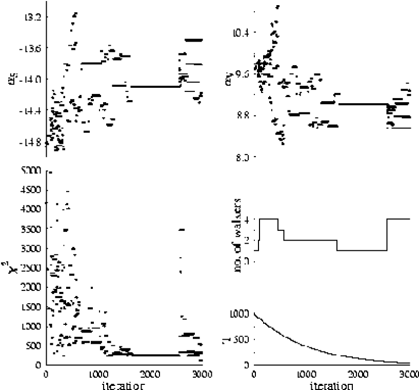
FIG. 1.: The upper two figures show the positions of the walkers in parameter space in $\alpha_{\rm S}$ and $\alpha_{\rm V}$ direction. For each walker, a dot is printed. The figure below on the left side shows the corresponding $\chi^{2}$ values. The other two figures indicate the size of the population and the external temperature.

FIG. 2.: Errors in percent for the observables binding energy, diffraction radius, surface thickness and rms charge radius for PC–F1 (filled diamonds) and NL–Z2 (open squares) are seen on the left. The right panels show the absolute mean errors for the corresponding observables, where the dashed lines indicate the chosen relative errors $\Delta O$ in the fitting procedure.

FIG. 3.: The left panel shows the energy per particle versus the vector density for the forces as indicated. On the right side, the effective nucleon mass (upper figure) and the scalar and vector mean-field potentials (lower figure) are drawn as emerging from the calculations.

FIG. 4.: Energy per particle versus neutron density for four RMF forces and the Skyrme force SLy6. The crosses mark data from Ref. [40].

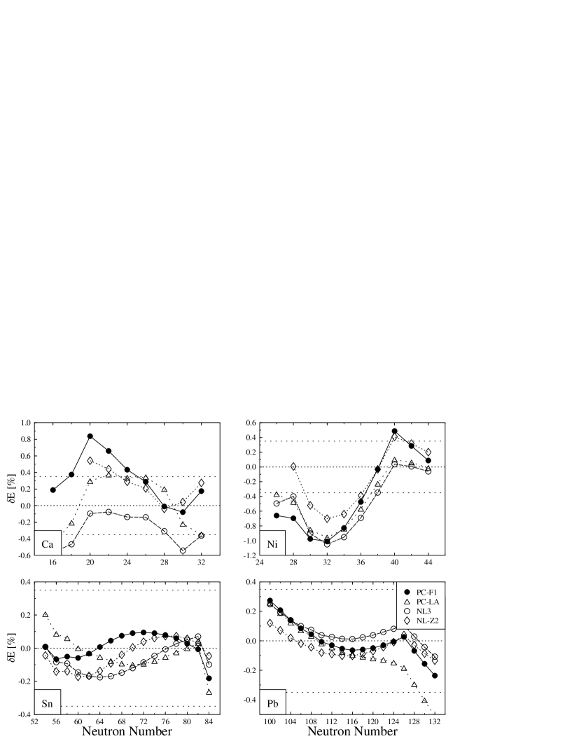
FIG. 5.: Deviation in % of the calculated energies from the experimental values in spherical calculations of isotopic chains. Note that the scales are different for each figure. The dotted lines indicate the accuracy that can be demanded from the models. The experimental errors are smaller than the size of the symbols used in the figure.

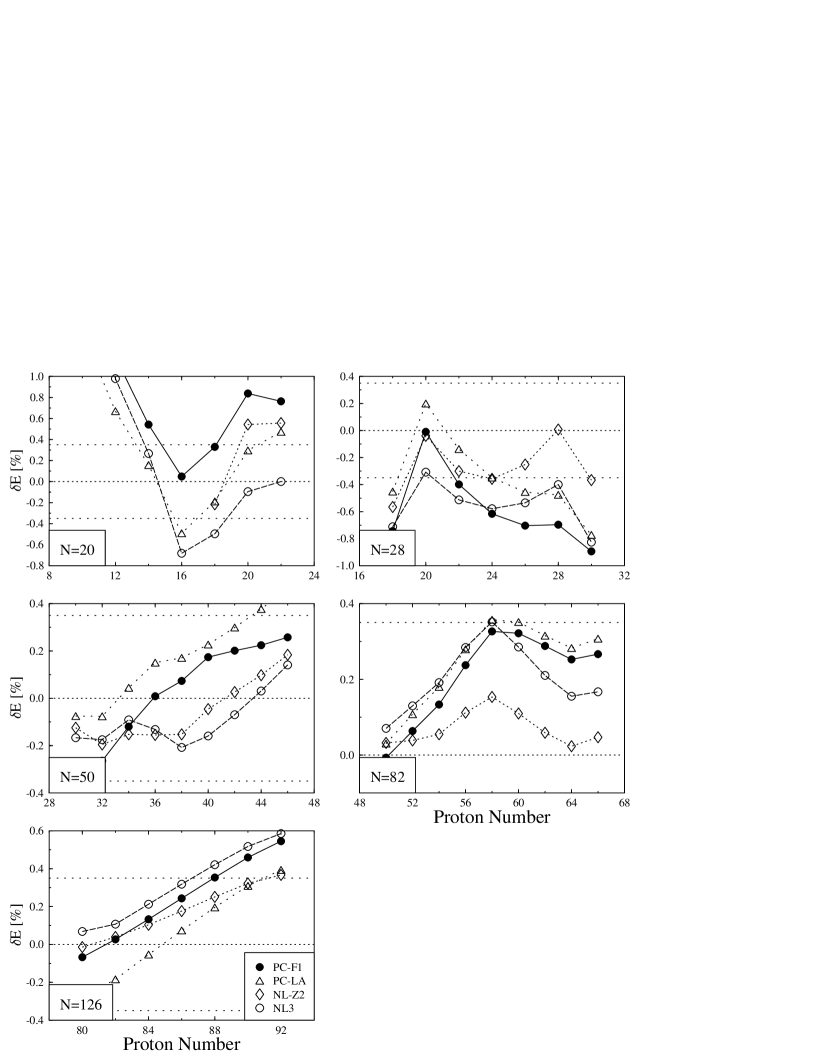
FIG. 6.: Deviation in % of the calculated energies from the experimental values in spherical calculations of isotonic chains. Note that the scales are different for each figure. The dotted lines indicate the accuracy demanded for energies. The experimental errors are smaller than the size of the symbols used in this figure.

FIG. 7.: Deviation in % of the calculated energies from the experimental values (upper figure) and ground-state deformations (lower figure) in axially deformed and reflection symmetric calculations. The errors for the binding energies are smaller than the size of the symbols used in this figure. The symbol with error bars indicates the measured ground-state deformation together with its uncertainty of ${}^{254}{\rm No}$ [43, 44].

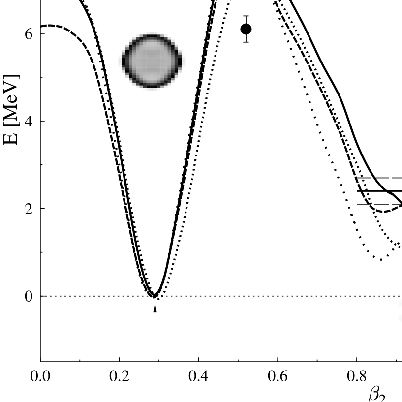
FIG. 8.: Fission barrier of ²⁴⁰Pu in axially- and reflection-asymmetric calculations with the forces as indicated. The experimental values for the ground-state deformation, the barrier height, and the energy of the second minimum are indicated, respectively, with an arrow, a symbol with error bars and three lines indicating the value and its errors. The data are taken from Ref. [46, 47, 48, 49].

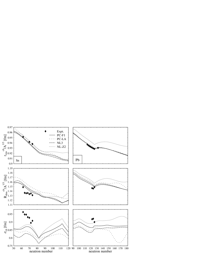
FIG. 9.: Surface thicknesses (lower figure), diffraction radii (middle) and rms charge radii (upper figure) for Sn (left) and Pb (right) isotopes emerging from spherical calculations. Note that the radii have been divided by $A^{1/3}$ to eliminate the liquid drop trend with mass number. The experimental data are from [29, 51, 52]. Their errors are smaller than the symbols used in this figure.

FIG. 10.: Total baryon densities of the nuclei ⁴⁸Ca and ¹⁰⁰Sn emerging from spherical calculations for the four RMF forces under consideration.

FIG. 11.: Formfactor of the charge density of the nucleus ⁴⁸Ca for the four RMF forces under consideration. The experimental data, which are taken from Ref. [55], are plotted in the momentum-transfer range $q=0.35-3.55~{}[{\rm fm^{-1}}]$, as in the original analysis.

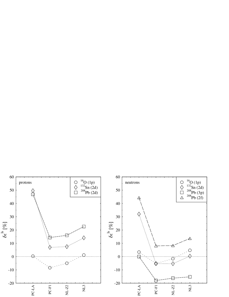
FIG. 12.: The percentage error in $ls$-splittings for protons (left) and for neutrons (right). The experimental errors are smaller than the size of the symbols used in these figures. The lines serve to guide the eye.

FIG. 13.: The neutron spin-orbit potential (upper figure) and effective mass (lower figure) in ²⁰⁸Pb for the forces under discussion.

observable	error	16O	88Sr	208Pb
$E_{\rm B}$	0.15 %	+	+	+
$r_{\rm rms}^{\rm ch}$	0.2 %	+	+	+
$\epsilon_{\rm ls}^{\rm p}$	5.0 %	+	+	+
$\epsilon_{\rm ls}^{\rm n}$	5.0 %	+	+	+

TABLE I.: Observables and chosen errors $\Delta O$ for set 1 of nuclei used for the SA fitting procedure. $E_{\rm B}$ denotes the binding energy, $r_{\rm rms}^{\rm ch}$ the rms charge radius and $\epsilon_{\rm ls}^{\rm p}$ and $\epsilon_{\rm ls}^{\rm n}$ the proton and neutron spin-orbit splittings of one selected level. A $+$ indicates an observable contributing to the total $\chi^{2}$. For the experimental values see Ref. [10].

observable	error	16O	40Ca	48Ca	56Ni	58Ni	88Sr	90Zr	100Sn	112Sn	120Sn	124Sn	132Sn	136Xe	144Sm	202Pb	208Pb	214Pb
$E_{\rm B}$	0.2 %	+	+	+	+	+	+	+	+	+	+	+	+	+	+	–	+	+
$R_{\mbox{dms}}$	0.5 %	+	+	+	–	+	+	+	–	+	+	+	–	–	–	–	+	–
$\sigma$	1.5 %	+	+	+	–	–	–	+	–	–	–	–	–	–	–	–	+	–
$r_{\mbox{rms}}^{\mbox{ch}}$	0.5 %	–	+	+	+	+	+	+	–	+	–	+	–	–	–	+	+	+
$\Delta_{\mbox{ p}}$	0.05 MeV	-	-	-	-	-	-	-	-	-	-	-	-	+	+	-	-	-
$\Delta_{\mbox{ n}}$	0.05 MeV	-	-	-	-	-	-	-	-	+	+	+	-	-	-	-	-	-

TABLE II.: Observables and chosen errors $\Delta O$ for set 2 of nuclei used for the Bevington fitting procedure. $R_{\rm diffr.}$ denotes the diffraction-radius, $\sigma$ the surface thickness, and $\Delta_{\rm p}$ and $\Delta_{\rm n}$ are the proton and neutron pairing gaps. A $+$ indicates an observable contributing to the total $\chi^{2}$. For the experimental values see Ref. [26]

coupling constant	value	dimension	uncorr. error [%]	corr. error [%]
$\alpha_{\rm S}$	$-3.83577\cdot 10^{-4}$	MeV-2	$2.6\cdot 10^{-3}$	$8.3\cdot 10^{-1}$
$\beta_{\rm S}$	$7.68567\cdot 10^{-11}$	MeV-5	$2.1\cdot 10^{-2}$	$4.7\cdot 10^{0}$
$\gamma_{\rm S}$	$-2.90443\cdot 10^{-17}$	MeV-8	$7.2\cdot 10^{-2}$	$1.4\cdot 10^{1}$
$\delta_{\rm S}$	$-4.1853\cdot 10^{-10}$	MeV-4	$2.0\cdot 10^{-1}$	$2.3\cdot 10^{1}$
$\alpha_{\rm V}$	$2.59333\cdot 10^{-4}$	MeV-2	$3.7\cdot 10^{-3}$	$1.2\cdot 10^{0}$
$\gamma_{\rm V}$	$-3.879\cdot 10^{-18}$	MeV-8	$4.4\cdot 10^{-1}$	$5.4\cdot 10^{1}$
$\delta_{\rm V}$	$-1.1921\cdot 10^{-10}$	MeV-4	$6.0\cdot 10^{-1}$	$7.6\cdot 10^{1}$
$\alpha_{\rm TV}$	$3.4677\cdot 10^{-5}$	MeV-2	$1.2\cdot 10^{0}$	$1.1\cdot 10^{1}$
$\delta_{\rm TV}$	$-4.2\cdot 10^{-11}$	MeV-4	$6.0\cdot 10^{1}$	$1.7\cdot 10^{3}$
$V_{\rm P}$	$-321$	MeV fm3	$1.3\cdot 10^{0}$	$2.0\cdot 10^{0}$
$V_{\rm N}$	$-308$	MeV fm3	$1.2\cdot 10^{0}$	$2.3\cdot 10^{0}$

TABLE III.: The set PC–F1 of coupling constants resulting from the final fitting procedure. In columns 4 and 5 the uncorrelated and correlated errors are shown as originating from the fitting procedure. Note that the values for the pairing strengths have been rounded according to the error marigins. The total $\chi^{2}$, $\chi^{2}$ per point and $\chi^{2}$ per degree of freedom are $\chi^{2}_{\rm tot}=99.1$, $\chi^{2}_{\rm pt}=2.11$, $\chi^{2}_{\rm df}=2.75$.

coupling constant	value	dimension	uncorr. error [%]	corr. error [%]
$\alpha_{\rm S}$	$-3.835821\cdot 10^{-4}$	MeV-2	$1.9\cdot 10^{-3}$	$8.1\cdot 10^{-1}$
$\beta_{\rm S}$	$7.6835\cdot 10^{-11}$	MeV-5	$1.6\cdot 10^{-2}$	$4.7\cdot 10^{0}$
$\gamma_{\rm S}$	$-2.91148\cdot 10^{-17}$	MeV-8	$5.2\cdot 10^{-2}$	$1.3\cdot 10^{1}$
$\delta_{\rm S}$	$-4.158\cdot 10^{-10}$	MeV-4	$2.6\cdot 10^{-1}$	$1.8\cdot 10^{1}$
$\alpha_{\rm V}$	$2.593511\cdot 10^{-4}$	MeV-2	$2.9\cdot 10^{-3}$	$1.3\cdot 10^{0}$
$\gamma_{\rm V}$	$-3.8234\cdot 10^{-18}$	MeV-8	$3.4\cdot 10^{-1}$	$5.2\cdot 10^{1}$
$\delta_{\rm V}$	$-1.218\cdot 10^{-10}$	MeV-4	$1.7\cdot 10^{0}$	$6.9\cdot 10^{1}$
$\alpha_{\rm TS}$	$2.34\cdot 10^{-6}$	MeV-2	$1.6\cdot 10^{1}$	$2.4\cdot 10^{3}$
$\alpha_{\rm TV}$	$3.241\cdot 10^{-5}$	MeV-2	$1.1\cdot 10^{0}$	$1.6\cdot 10^{2}$
$\delta_{\rm TV}$	$-6.0\cdot 10^{-11}$	MeV-4	$2.5\cdot 10^{1}$	$3.7\cdot 10^{2}$
$V_{\rm P}$	$-321$	MeV fm3	$8.7\cdot 10^{-1}$	$1.6\cdot 10^{0}$
$V_{\rm N}$	$-308$	MeV fm3	$8.1\cdot 10^{-1}$	$1.3\cdot 10^{0}$

TABLE IV.: The set PC–F2 of coupling constants emerging from the fitting procedure including the linear isovector-scalar term. In columns 4 and 5 the uncorrelated and correlated errors are shown as originating from the fitting procedure. The total $\chi^{2}$, $\chi^{2}$ per point and $\chi^{2}$ per degree of freedom are $\chi^{2}_{\rm tot}=98.5$, $\chi^{2}_{\rm pt}=2.10$, $\chi^{2}_{\rm df}=2.80$.

coupling constant	value	dimension	uncorr. error [%]	corr. error [%]
$\alpha_{\rm S}$	$-3.835796\cdot 10^{-4}$	MeV-2	$2.5\cdot 10^{-3}$	$9.9\cdot 10^{-1}$
$\beta_{\rm S}$	$7.6853\cdot 10^{-11}$	MeV-5	$2.0\cdot 10^{-2}$	$5.3\cdot 10^{0}$
$\gamma_{\rm S}$	$-2.9062\cdot 10^{-17}$	MeV-8	$6.9\cdot 10^{-2}$	$1.7\cdot 10^{1}$
$\delta_{\rm S}$	$-4.1797\cdot 10^{-10}$	MeV-4	$2.1\cdot 10^{-1}$	$2.4\cdot 10^{1}$
$\alpha_{\rm V}$	$2.593357\cdot 10^{-4}$	MeV-2	$3.5\cdot 10^{-3}$	$1.7\cdot 10^{0}$
$\gamma_{\rm V}$	$-3.8731\cdot 10^{-18}$	MeV-8	$4.4\cdot 10^{-1}$	$5.9\cdot 10^{1}$
$\delta_{\rm V}$	$-1.1997\cdot 10^{-10}$	MeV-4	$6.9\cdot 10^{-1}$	$8.0\cdot 10^{1}$
$\alpha_{\rm TV}$	$3.549\cdot 10^{-5}$	MeV-2	$1.2\cdot 10^{0}$	$7.6\cdot 10^{0}$
$\gamma_{\rm TV}$	$-5.4\cdot 10^{-17}$	MeV-8	$5.7\cdot 10^{1}$	$1.8\cdot 10^{2}$
$\delta_{\rm TV}$	$-4.0\cdot 10^{-11}$	MeV-4	$1.1\cdot 10^{2}$	$4.0\cdot 10^{2}$
$V_{\rm P}$	$-321$	MeV fm3	$1.4\cdot 10^{0}$	$1.7\cdot 10^{0}$
$V_{\rm N}$	$-308$	MeV fm3	$1.2\cdot 10^{0}$	$1.3\cdot 10^{0}$

TABLE V.: The set PC–F3 of coupling constants emerging from the fitting procedure including the nonlinear term in the isovector-vector density. In columns 4 and 5 the uncorrelated and correlated errors are shown as originating from the fitting procedure. The total $\chi^{2}$, $\chi^{2}$ per point and $\chi^{2}$ per degree of freedom are $\chi^{2}_{\rm tot}=98.8$, $\chi^{2}_{\rm pt}=2.10$, $\chi^{2}_{\rm df}=2.82$.

coupling constant	value	dimension	uncorr. error [%]	corr. error [%]
$\alpha_{\rm S}$	$-3.83564\cdot 10^{-4}$	MeV-2	$2.9\cdot 10^{-3}$	$1.0\cdot 10^{0}$
$\beta_{\rm S}$	$7.6806\cdot 10^{-11}$	MeV-5	$2.0\cdot 10^{-2}$	$5.7\cdot 10^{0}$
$\gamma_{\rm S}$	$-2.9105\cdot 10^{-17}$	MeV-8	$6.9\cdot 10^{-2}$	$1.9\cdot 10^{1}$
$\delta_{\rm S}$	$-4.16057\cdot 10^{-10}$	MeV-4	$2.1\cdot 10^{-1}$	$2.3\cdot 10^{1}$
$\alpha_{\rm V}$	$2.593614\cdot 10^{-4}$	MeV-2	$3.5\cdot 10^{-3}$	$1.5\cdot 10^{0}$
$\gamma_{\rm V}$	$-3.844\cdot 10^{-18}$	MeV-8	$4.4\cdot 10^{-1}$	$6.8\cdot 10^{1}$
$\delta_{\rm V}$	$-1.2154\cdot 10^{-10}$	MeV-4	$6.8\cdot 10^{-1}$	$7.6\cdot 10^{1}$
$\alpha_{\rm TS}$	$-5.92\cdot 10^{-6}$	MeV-2	$7.8\cdot 10^{0}$	$6.8\cdot 10^{3}$
$\delta_{\rm TS}$	$-1.12\cdot 10^{-10}$	MeV-4	$4.1\cdot 10^{1}$	$8.4\cdot 10^{2}$
$\alpha_{\rm TV}$	$3.937\cdot 10^{-5}$	MeV-2	$1.0\cdot 10^{0}$	$8.9\cdot 10^{1}$
$\delta_{\rm TV}$	$3.0\cdot 10^{-12}$	MeV-4	$1.5\cdot 10^{3}$	$3.1\cdot 10^{4}$
$V_{\rm P}$	$-321$	MeV fm3	$1.4\cdot 10^{0}$	$1.5\cdot 10^{0}$
$V_{\rm N}$	$-308$	MeV fm3	$1.2\cdot 10^{0}$	$1.4\cdot 10^{0}$

TABLE VI.: The set PC-F4 of eleven coupling constants emerging from the fitting procedure including 4 isovector coupling constants. In columns 4 and 5 the uncorrelated and correlated errors are shown as originating from the fitting procedure. The total $\chi^{2}$, $\chi^{2}$ per point and $\chi^{2}$ per degree of freedom are $\chi^{2}_{\rm tot}=98.2$, $\chi^{2}_{\rm pt}=2.09$, $\chi^{2}_{\rm df}=2.89$.

coupling constant	value from NL–Z2	PC–F1	PC–F2	PC–F3	PC–F4
$\alpha_{\rm S}$ [MeV]-2	$-4.225\cdot 10^{-4}$	$-3.836\cdot 10^{-4}$	$-3.836\cdot 10^{-4}$	$-3.836\cdot 10^{-4}$	$-3.836\cdot 10^{-4}$
$\delta_{\rm S}$ [MeV]-4	$-1.737\cdot 10^{-9}$	$-4.185\cdot 10^{-10}$	$-4.158\cdot 10^{-10}$	$-4.180\cdot 10^{-10}$	$-4.161\cdot 10^{-10}$
$\alpha_{\rm V}$ [MeV]-2	$2.739\cdot 10^{-4}$	$2.593\cdot 10^{-4}$	$2.594\cdot 10^{-4}$	$2.593\cdot 10^{-4}$	$2.594\cdot 10^{-4}$
$\delta_{\rm V}$ [MeV]-4	$4.502\cdot 10^{-10}$	$-1.192\cdot 10^{-10}$	$-1.218\cdot 10^{-10}$	$-1.120\cdot 10^{-10}$	$-1.215\cdot 10^{-10}$
$\alpha_{\rm TV}$ [MeV]-2	$3.566\cdot 10^{-5}$	$3.468\cdot 10^{-5}$	$3.241\cdot 10^{-5}$	$3.549\cdot 10^{-5}$	$3.937\cdot 10^{-5}$
$\delta_{\rm TV}$ [MeV]-4	$6.125\cdot 10^{-11}$	$-4.20\cdot 10^{-11}$	$-6.0\cdot 10^{-11}$	$-4.0\cdot 10^{-11}$	$3.0\cdot 10^{-12}$
$\alpha_{\rm TS}$ [MeV]-2	–	–	$2.34\cdot 10^{-6}$	–	$-5.92\cdot 10^{-6}$
$\delta_{\rm TS}$ [MeV]-4	–	–	–	–	$-1.12\cdot 10^{-10}$

TABLE VII.: Coupling constants from the RMF-FR interaction NL-Z2 and corresponding values from the RMF-PC interactions PC-F1 to PC-F4.

	PC–F1	PC–LA	NL-Z2	NL3	SLy6	SkI3
$\rho_{0}$ (fm-3)	$0.151$	0.148	0.151	0.148	0.159	0.158
$E/A$ (MeV)	$-16.17$	-16.126	-16.07	-16.24	-15.90	-15.96
$m^{*}/m$	0.61	0.575	0.583	0.595	0.690	0.577
$K$ (MeV)	270	264	172	272	230	258
$a_{\rm sym}$ (MeV)	37.8	37.194	39.0	37.4	32.0	34.8

TABLE VIII.: Bulk properties of nuclear matter for the forces under consideration

Coupling Constant	$c_{ln}(\rm{PC-F1})$	$c_{ln}(\rm{PC-F2})$	$c_{ln}(\rm{PC-F3})$	$c_{ln}(\rm{PC-F4})$	Order in $\Lambda$
$\alpha_{S}$	-1.641	-1.641	-1.641	-1.641	$\Lambda^{0}$
$\beta_{S}$	1.443	1.443	1.443	1.442	$\Lambda^{-1}$
$\gamma_{S}$	-2.695	-2.701	-2.696	-2.700	$\Lambda^{-2}$
$\delta_{S}$	-1.061	-1.054	-1.060	-1.055	$\Lambda^{-2}$
$\alpha_{V}$	1.109	1.109	1.109	1.109	$\Lambda^{0}$
$\gamma_{V}$	-0.360	-0.355	-0.359	-0.357	$\Lambda^{-2}$
$\delta_{V}$	-0.302	-0.309	-0.304	-0.308	$\Lambda^{-2}$
$\alpha_{TS}$	–	0.040	–	-0.101	$\Lambda^{0}$
$\delta_{TS}$	–	–	–	-1.134	$\Lambda^{-2}$
$\alpha_{TV}$	0.593	0.555	0.607	0.674	$\Lambda^{0}$
$\gamma_{TV}$	–	–	-80.470	–	$\Lambda^{-2}$
$\delta_{TV}$	-0.422	-0.612	-0.404	0.026	$\Lambda^{-2}$
# $c_{ln}$	9	10	10	11
# natural	9	9	9	9
$|\rm{max}|/|\rm{min}|$	8.92	67.5	264.7	103.8
$\chi^{2}_{df}$	2.75	2.80	2.82	2.89

TABLE IX.: QCD-Scaled Coupling Constants for Four Relativistic Point Coupling Interactions.

REFERENCES

- [1] B. D. Serot and J. D. Walecka, Phys. Lett. 87B, 172 (1979).
- [2] C. J. Horowitz and B. D. Serot, Nucl. Phys. A368, 503 (1981).
- [3] B. D. Serot and J. D. Walecka, Advances in Nuclear Physics, vol. 16 (Plenum Press, 1986).
- [4] M. Rufa, P. G. Reinhard, J. A. Maruhn, W. Greiner, and M. R. Strayer, Phys. Rev. C 38, 390 (1988).
- [5] P. G. Reinhard, Rep. Prog. Phys. 52, 439 (1989).
- [6] Y. K. Gambhir, P. Ring, and A. Thimet, Ann. Phys. 198, 132 (1990).
- [7] R. J. Furnstahl, B. D. Serot, and H. B. Tang, Nucl. Phys. A615, 441 (1997).
- [8] G. A. Lalazissis, J. Konig, and P. Ring, Phys. Rev. C 55, 540 (1997).
- [9] R. J. Furnstahl and J. J. Rusnak, Nucl. Phys. A632, 607 (1998).
- [10] B. A. Nikolaus, T. Hoch, and D. G. Madland, Phys. Rev. C 46, 1757 (1992).
- [11] T. Hoch, D. Madland, P. Manakos, T. Mannel, B. A. Nikolaus, and D. Strottman, Phys. Rep. 242, 253 (1994).
- [12] J. J. Rusnak and R. J. Furnstahl, Nucl. Phys. A627, 495 (1997).
- [13] P. Manakos and T. Mannel, Z. Phys. A 330, 223 (1988).
- [14] P. Manakos and T. Mannel, Z. Phys. A 334, 481 (1989).
- [15] J. A. Maruhn, T. Burvenich, and D. G. Madland, J. Comput. Phys. 169, 238 (2001).
- [16] S. P. Klevansky, Rev. Mod. Phys. 64, 649 (1992).
- [17] S. Weinberg, Phys. Lett. B 251, 288 (1990).
- [18] P. Quentin and H. Flocard, Ann. Rev. Nucl. Part. Sci. 21, 523 (1978).
- [19] J. Friedrich and P.-G. Reinhard, Phys. Rev. C 33, 355 (1986).
- [20] P.-G. Reinhard and H. Flocard, Nucl. Phys. A 584, 467 (1995).
- [21] J. L. Friar, D. G. Madland, and B. W. Lynn, Phys. Rev. C 53, 3085 (1996).
- [22] D. G. Madland, in International Conference on Nuclear Data for Science and Technology (Italian Physical Society, Bologna, 1997), vol. 1, p. 77.
- [23] M. E. J.D. Perdew, K. Burke, Phys. Rev. Lett. 77, 3865 (1996).
- [24] Y. Sugahara and H. Toki, Nucl. Phys. A 579, 557 (1994).
- [25] J. D. Bjorken and S. D. Drell, Relativistic Quantum Fields (McGraw-Hill, New-York, 1965).
- [26] M. Bender, K. Rutz, P.-G. Reinhard, J. A. Maruhn, and W. Greiner, Phys. Rev. C 60, 34304 (1999).
- [27] M. Bender, K. Rutz, P.-G. Reinhard, and J. A. Maruhn, Eur. Phys. J. A 8, 59 (2000).
- [28] M. Bender, K. Rutz, P.-G. Reinhard, and J. A. Maruhn, Eur. Phys. J. A 7, 467 (2000).
- [29] J. Friedrich and N. Vögler, Nucl. Phys. A 373, 192 (1982).
- [30] P. G. Reinhard and R. Y. Cusson, Nucl. Phys. A 378, 418 (82).
- [31] P. R. Bevington and D. K. Robinson, Data Reduction and Error Analysis for the Physical Sciences, second edition (WCB/McGraw-Hill, 1992).
- [32] M. Rufa, P. G. Reinhard, J. A. Maruhn, W. Greiner, and M. Strayer, Phys. Rev. C 38, 390 (1988).
- [33] W. H. Press, S. A. Teukolsky, W. T. Vettering, and B. P. Flannery, Numerical Recipes in C (Cambridge University Press, 1988).
- [34] J. Thijssen, Computational Physics (Cambridge University Press, 1999).
- [35] M. Bender, K. Rutz, P.-G. Reinhard, and J. A. Maruhn, Eur. Phys. J. A 8, 59 (2000).
- [36] G. Lalazissis, J. König, and P. Ring, Phys. Rev. C 55, 540 (1997).
- [37] E. Chabanat, Interactions effectives pour des conditions extremes d’isospin, Ph.D. thesis, Universite Claude Bernard Lyon-1 (1995).
- [38] W. D. Myers, Droplet Model of Atomic Nuclei (Plenum, New-York, 1977).
- [39] F. Tondeur, S. Goriely, J. M. Pearson, and M. Onsi, Phys. Rev. C 62, 024308 (2000).
- [40] B. Friedmann and V. Pandharipande, Nucl. Phys. A 361, 502 (1981).
- [41] W. Satula and R. Wyss, Phys. Lett. B 393, 1 (1997).
- [42] T. Bürvenich, K. Rutz, M. Bender, P.-G. Reinhard, J. A. Maruhn, and W. Greiner, Eur. Phys. J. A 3, 139 (1998).
- [43] P. Reiter et al., Phys. Rev. Lett. 82, 509 (1999).
- [44] M. Leino, Eur. Phys. Journ. A 6, 63 (1999).
- [45] K. Rutz, J. A. Maruhn, P.-G. Reinhard, and W. Greiner, Nucl. Phys. A 590, 680 (1995).
- [46] S. Bjørnholm and J. E. Lynn, Rev. Mod. Phys. 52, 725 (1980).
- [47] R. B. Firestone, V. S. Shirley, S. Y. F. Chu, C. M. Baglin, and J. Zipkin, Table of Isotopes (John Wiley & Sons New York, 1996).
- [48] K. E. G. Löbner, M. Vetter, and V. Hönig, Nucl. Data Tables A 7, 495 (1970).
- [49] C. E. Bemis Jr., F. K. McGowan, J. L. C. Ford Jr., W. T. Milner, P. H. Stelson, and R. L. Robinson, Phys. Rev. C 8, 1466 (1973).
- [50] P.-G. Reinhard and K. Goeke, Lecture Notes in Physics 89, 440 (1979).
- [51] E. W. Otten, Treatise on Heavy-Ion Science (D. A. Bromley ed.) vol. VIII (Plenum Press New York and London, 1989).
- [52] G. Fricke, C. Bernhardt, K. Heilig, L. A. Schaller, L. Schellenberg, E. B. Sherba, and C. W. D. Jaeger, At. Data Nucl. Data Tables 60, 177 (1995).
- [53] M. M. Sharma, G. Lalazissis, J. Koenig, and P. Ring, Phys. Rev. Lett. 74, 3744 (1995).
- [54] P.-G. Reinhard, Phys.Lett. A 169, 281 (1992).
- [55] H. de Vries, C. W. de Jager, and C. de Vries, Atomic Data and Nuclear Data Tables 36, 495 (1987).
- [56] K. Rutz, M. Bender, P.-G. Reinhard, J. Maruhn, and W. Greiner, Nucl. Phys. A 634, 67 (1998).
- [57] K. Rutz, M. Bender, T. Bürvenich, T. Schilling, P.-G. Reinhard, J. A. Maruhn, and W. Greiner, Phys. Rev. C 56, 238 (1997).
- [58] J. Decharge, J.-F. Berger, K. Dietrich, and M. S. Weiss, Phys. Lett. B 451, 275 (1999).
- [59] J.-F. Berger, L. Bitaud, J. Decharge, M. Girod, and K. Dietrich, Nucl. Phys. A 685, 1c (2001).
- [60] A. Manohar and H. Georgi, Nucl. Phys. B234, 189 (1984).
- [61] S. Weinberg, Physica 96A, 327 (1979).
- [62] B. W. Lynn, Nucl. Phys. B402, 281 (1993).
- [63] R. Machleidt, in M. B. Johnson and A. Picklesimer, eds., Relativistic Dynamics and Quark-Nuclear Physics (Wiley, New York, 1986), p. 71.