IFUP-TH 44/00

Coulomb-Nuclear Coupling and Interference Effects in the Breakup of Halo Nuclei

Abstract

Nuclear and Coulomb breakup of halo nuclei have been treated often as incoherent processes and structure information have been extracted from their study. The aim of this paper is to clarify whether interference effects and Coulomb-nuclear couplings are important and how they could modify the simple picture previously used. We calculate the neutron angular and energy distributions by using first order perturbation theory for the Coulomb amplitude and an eikonal approach for the nuclear breakup. This allows for a simple physical interpretation of the results which are mostly analytical. Our formalism includes the effect of the nuclear distortion of the neutron wave function on the Coulomb amplitude. This leads to a Coulomb-nuclear coupling term derived here for the first time which gives a small contribution for light targets but is of the same order of magnitude as nuclear breakup for heavy targets. The overall interference is constructive for light to medium targets and destructive for heavy targets. Thus it appears that Coulomb breakup experiments need to be analyzed with more accurate models than those used so far.

PACS number(s):25.70.Hi, 21.10Gv,25.60Ge,25.70Mn,27.20+n

Key-words Nuclear breakup, Coulomb breakup, interference, halo nuclei.

1 Introduction

This paper is concerned with the nuclear and Coulomb breakup of weakly bound nuclei, in particular halo nuclei in which the last neutron is very weakly bound and in a state of low angular momentum. As a consequence its distance from the core center is quite large and this makes the nuclear and Coulomb breakup strong effects in particular when the target is heavy.

There have been a large number of approaches [1]-[65] attempting to give an accurate description of this phenomenon and the most recent papers contain a review of the present situation [1, 2, 3]. The accuracy of the method is an important issue not only from the point of view of the understanding of the reaction mechanism but also because a number of parameters of the neutron initial state wave function such as the binding energy and the spectroscopic factor can be deduced from the data analysis [1]-[8].

An important aspect of the problem is that nuclear breakup is always present at the same time. It is dominant for a light target and it remains non negligible for heavy targets. Its contribution to the total breakup cross section on a heavy target has been a matter of debate but it should range from about 20% to 50%. In such conditions one expects to see interference effects. However most of the analysis of experimental data so far performed have relied on the assumption that interference effects are small in the intermediate energy range (40-80 A.MeV). Furthermore nuclear and Coulomb breakup have been treated as independent processes and calculated in the absence of each other to different orders in the interactions. Such approximations have been justified by the fact that the nuclear interaction is strong and has a short range, therefore needs to be treated to all orders. The Coulomb potential on the other hand is comparatively weaker and has a long range, therefore it has often been treated to first order.

One difficulty in the theoretical approach comes from the fact that one needs to have a consistent description of the nuclear and Coulomb breakup amplitudes from which the interference originates. In this respect the most accurate calculations presently available are the numerical solutions of the Schrödinger equation [2]. They treat both interactions to all orders and therefore contain also all possible interference effects. However it is not so easy to extract from them a simple picture of the coupling mechanisms. The numerical solution of the Schrödinger equation has also been used with only the nuclear [9] or the Coulomb potential [10, 11, 12] to test the accuracy of simpler models used to calculate the nuclear and Coulomb breakup separately. The conclusions of recent works have been that, for well developed haloes, nuclear breakup needs to be treated to all orders but the sudden and eikonal approximations are acceptable since they give an accuracy of about 20% [9, 13] compatible with the present experimental error bars. On the other hand it seems that Coulomb breakup can be safely treated to first order [1, 2, 10], but the time dependence needs to be retained in order to reproduce some very fine experimental observables such as the neutron-core final energy spectrum. DWBA [14, 15, 16], semiclassical [17, 18, 19], adiabatic [20] and coupled channel [21] approaches have also been proposed. A common feature of some of those approaches [2, 12, 18, 19] has been to give a smaller Coulomb breakup contribution than that calculated with the first order perturbation theory. Also many of them were concerned with proton breakup [21, 22] and lower energy regimes. Such situations are physically more challenging and we do not attempt to include them in the present discussion. Therefore we restrict ourselves to neutron breakup at intermediate energies in the attempt to clarify the role of Coulomb-nuclear couplings and interference and to make a link between numerical solutions and simple analytical methods.

An important issue is to determine the experimental observable on which couplings and interference effects would show up best. Interferences are a quantum mechanical manifestation of a coherence effect. Therefore in order to see them an observable of the ”exclusive” type is expected to be most suitable. Some work has been done [17, 21, 23, 24] to study interference effects on the ejectile angular distribution but nothing exists at present on the interference effects on the neutron angular distribution which we address here. Neutron angular distributions have been the best experimental proof of the existence of the two distinct mechanisms of Coulomb and nuclear diffractive breakup. Furthermore they give information on the relative strength of the two processes, on the target dependence and beam energy dependence of the reaction mechanisms.

Neutron angular distributions due to nuclear and Coulomb breakup were measured and calculated in [25] but information on the interferences were not extracted. Another reliable calculation of the neutron angular distribution from nuclear breakup alone was given in [26]. Models for the reaction mechanism and structure information extracted from the data can be considered reliable only if three aspects of the data are reproduced at the same time within a given model. One is the ejectile or neutron energy spectrum or its equivalent parallel momentum distribution. Another is the neutron angular distribution. Finally the absolute breakup cross section is important to fix the initial state parameters.

In this paper we will try to get some insight on the problem by a simple but consistent calculation of the Coulomb and the nuclear breakup in the presence of each other and of their interference. This will allow us to get both the neutron angular distribution as well as its energy spectrum due to the combined effects of the nuclear and Coulomb interaction. The absolute breakup cross section is obtained from the integration of the angular distribution. We will discuss under which experimental conditions interference effects could be seen and why they have not been clearly identified so far. An important result of our method is that it gives simple analytical expressions for the Coulomb cross section for any initial angular momentum state of the neutron.

Section 2 of the paper presents some theoretical background. The purpose is to clarify the assumptions made in deriving the nuclear and Coulomb breakup amplitudes. Section 3 gives expressions for the cross-section and the breakup amplitudes. The results of calculations are presented in section 4 and conclusions in section 5. Some details of the derivation of the Coulomb amplitude are given in the first Appendix. The calculations presented in the paper assume an s-state initial neutron wave function in the projectile. Some formulae which generalize the results for the Coulomb amplitude are given in the second appendix. They are included for completeness and are not used in the present paper.

2 Theoretical background

We consider the breakup of a halo nucleus like ¹¹Be consisting of a neutron bound to a ¹⁰Be core in a collision with a target nucleus. In previous works on halo breakup [26, 27] we have assumed that the projectile core and the target move along classical trajectories. Here we adopt a different approach. The system of the halo nucleus and the target is described by Jacobi coordinates $\left(\mathbf{R,r}\right)$ where $\mathbf{R}$ is the position of the center of mass of the halo nucleus relative to the target nucleus and $\mathbf{r}$ is the position of the neutron relative to the halo core, and the coordinate $\mathbf{R}$ is assumed to move on a classical path. This allows target recoil to be included in a consistent way. The Hamiltonian of the system is

$$H=T_{R}+T_{r}+V_{nc}\left(\mathbf{r}\right)+V_{2}\left(\mathbf{R,r}\right)$$ (1)

where $T_{R}$ and $T_{r}$ are the kinetic energy operators associated with the coordinates $\mathbf{R}$ and $\mathbf{r}$ and $V_{nc}$ is a real potential describing the interaction of the neutron with the core. The potential $V_{2}$ describes the interaction between the projectile and the target. It is a sum of two parts depending on the relative coordinates of the neutron and the target and of the core and the target

$$V_{2}\left(\mathbf{R,r}\right)=V_{nt}\left(\mathbf{\beta}_{2}\mathbf{r+R}\right)+V_{ct}\left(\mathbf{R-\beta}_{1}\mathbf{r}\right)$$ (2)

Here $\beta_{1}=m_{n}/m_{p}$, $\beta_{2}=m_{c}/m_{p}=1-\beta_{1}$, where $m_{n}$ is the neutron mass, $m_{c}$ is the mass of the projectile core and $m_{p}=m_{n}+m_{c}$ is the projectile mass. Both $V_{nt}$ and $V_{ct}$ are represented by complex optical potentials. The imaginary part of $V_{nt}$ describes absorption of the neutron by the target to form a compound nucleus. It gives rise to the stripping part of the halo breakup. The imaginary part of $V_{ct}$ describes reactions of the halo core with the target. The potential $V_{ct}$ also includes the Coulomb interaction between the halo core and the target. This part of $V_{ct}$ is responsible for Coulomb breakup.

The mass ratio $\beta_{1}$ is small for a halo nucleus with a heavy core. For example $\beta_{1}\approx 0.1$ and $\beta_{2}\approx 0.9$ in the case of ¹¹Be. This property is used here to approximate the neutron-target and neutron-core potentials by

$$V_{nt}\left(\mathbf{\beta}_{2}\mathbf{r+R}\right) \approx V_{nt}(\mathbf{r+R)}$$ (3)

$$V_{ct}\left(\mathbf{R-\beta}_{1}\mathbf{r}\right) \approx V_{ct}(\mathbf{R})\mathbf{+V}_{eff}\left(\mathbf{r,R}\right)$$ (4)

where

$$\mathbf{V}_{eff}\left(\mathbf{r,R}\right)=\mathbf{\beta}_{1}\mathbf{r\cdot F}_{ct}\left(\mathbf{R}\right)\qquad\mathrm{and}\qquad\mathbf{F}_{ct}\left(\mathbf{R}\right)=-\nabla V_{ct}\left(\mathbf{R}\right)$$ (5)

Here  $\mathbf{F}_{ct}\left(\mathbf{R}\right)$ is the classical force acting between the target and the projectile core. The halo breakup is caused by the direct neutron target interaction $V_{nt}$ or by a recoil effect due to the core-target interaction. Coulomb breakup of a one-neutron halo nucleus is a recoil effect due the Coulomb component $V_{ct}$ of the core-target interaction and is contained in $\mathbf{V}_{eff}\left(\mathbf{r,R}\right)$. It is proportional to the mass ratio $\beta_{1}$. The dipole expansion Eqs.(4),(5) is a good approximation provided $\beta_{1}r<<R$. In the case considered here $r$ is of the order of the halo radius (4 to 6 fm) and $R$ is larger than the core-target strong absorption radius ( about 6 fm for a ⁹Be target and 12 fm for a Pb target). As $\beta_{1}\approx 0.1$  for the ¹¹Be halo nucleus the dipole approximation should be valid.

The nuclear part of the core-target interaction can also contribute to $\mathbf{V}_{eff}$ and gives rise to the ’shake-off’ component of the breakup amplitude which is discussed in ref.[28]. They show that it can be important for a light target. It is not included in the present paper.

The theory in this paper is based on a time dependent approach which can be derived from an eikonal approximation. The projectile motion relative to the target is described by a time-dependent classical trajectory $\mathbf{R}\left(t\right)=\mathbf{d}+vt\mathbf{\hat{z}}$ with constant velocity $v$ and impact parameter $\mathbf{d}$ ( $\mathbf{\hat{z}}$ is a unit vector parallel to the z-axis). With the approximations (3,4) and (5) to the potentials the wave function $\phi\left(\mathbf{r,d},t\right)$ describing the dynamics of the halo neutron satisfies the time-dependent equation

$$i\hbar\frac{\partial\phi\left(\mathbf{r,}\mathbf{d},t\right)}{\partial t}=\left(H_{r}+V_{nt}(\mathbf{r+R}\left(t\right)\mathbf{)+V}_{eff}\left(\mathbf{r,R}\left(t\right)\right)\right)\phi\left(\mathbf{r,}\mathbf{d},t\right)$$ (6)

where $H_{r}=T_{r}+V_{nc}\left(\mathbf{r}\right)$ is the Hamiltonian for the halo nucleus. As $t\rightarrow-\infty$ the wave function tends to the initial halo nucleus wave-function

$$\phi\left(\mathbf{r,}\mathbf{d},t\right)\rightarrow\phi_{lm}\left(\mathbf{r},t\right)=\phi_{lm}\left(\mathbf{r}\right)\exp\left(-i\varepsilon_{0}t/\hbar\right)$$ (7)

with binding energy $\varepsilon_{0}$. The initial state $\phi_{lm}\left(\mathbf{r}\right)$ can be an s-state or a general single particle state with angular momentum $\left(l,m\right)$.

In the present paper we neglect the final state interactions between the neutron and the halo core, but include the final state interactions between the neutron and the target. This approximation should be satisfactory unless there are resonances in the neutron-core final state interaction which give rise to modification in the momentum distributions of the fragments of the type recently discussed in [9]. Such effects have not been seen so far in the experimental distributions. When the neutron-core final state interactions are neglected the breakup amplitude can be written as

$$g_{lm}\left(\mathbf{k,}\mathbf{d}\right)=\frac{1}{i\hbar}\int_{-\infty}^{\infty}dt\left\langle\phi_{f}\left(t\right)|\bar{V}_{2}\left(\mathbf{r},t\right)|\phi_{lm}\left(t\right)\right\rangle$$ (8)

where $\bar{V}_{2}\left(\mathbf{r,}t\right)=V_{nt}(\mathbf{r+R}\left(t\right)\mathbf{)+V}_{eff}\left(\mathbf{r,R}\left(t\right)\right)$ and $\phi_{f}\left(t\right)$ satisfies the equation

$$i\hbar\frac{\partial\phi_{f}\left(t\right)}{\partial t}=(T_{r}+\bar{V}_{2}\left(\mathbf{r},t\right))\phi_{f}\left(t\right)$$ (9)

with the boundary condition that $\phi_{f}\left(t\right)\sim\exp\left(i\mathbf{k\cdot r}-i\varepsilon_{\mathbf{k}}t/\hbar\right)$ when $t$ is large. The final step is to make an eikonal approximation for $\phi_{f}\left(t\right)$

$$\phi_{f}\left(t\right)=\exp\left(i\mathbf{k\cdot r}-i\varepsilon_{\mathbf{k}}t/\hbar\right)\exp\left(-\frac{1}{i\hbar}\int_{t}^{\infty}\bar{V}_{2}\left(\mathbf{r},t^{\prime}\right)dt^{\prime}\right)$$ (10)

The breakup amplitude becomes

$$g_{lm}\left(\mathbf{k,}\mathbf{d}\right)=\frac{1}{i\hbar}\int d^{3}\mathbf{r}\int dte^{-i\mathbf{k\cdot r}+i\omega t}e^{\left(\frac{1}{i\hbar}\int_{t}^{\infty}\bar{V}_{2}\left(\mathbf{r},t^{\prime}\right)dt^{\prime}\right)}\bar{V}_{2}\left(\mathbf{r},t\right)\phi_{lm}\left(\mathbf{r}\right)$$ (11)

where $\omega=\left(\varepsilon_{\mathbf{k}}-\varepsilon_{0}\right)/\hbar$.

The components $V_{nt}$ and $V_{eff}$ of $\bar{V}_{2}\left(\mathbf{r},t\right)$ have to be treated differently because of the long range of the Coulomb interaction in $V_{eff}$. The neutron-target interaction is strong and has a short range. In this paper we assume that the interaction time $\tau_{f}$ for this part of the interaction is very short in the sense that $\omega\tau_{f}$ is small compared with unity. On the other hand the dominant contribution to $V_{eff}$ comes from the long range Coulomb interaction between the halo core and the target. It is weaker and changes more slowly. In this paper we calculate the contribution of $V_{eff}$ to first order but include its full time dependence. We will show that under such hypothesis the total amplitude $g_{lm}\left(\mathbf{k,}\mathbf{d}\right)$ can be written as a sum of two parts

$$g_{lm}\left(\mathbf{k,}\mathbf{d}\right)=g_{lm}^{nucl}\left(\mathbf{k,}\mathbf{d}\right)+g_{lm}^{Coul}\left(\mathbf{k,}\mathbf{d}\right)$$ (12)

where $g_{lm}^{nucl}\left(\mathbf{k,}\mathbf{d}\right)$ is zero order in $V_{eff}$ and $g_{lm}^{Coul}\left(\mathbf{k,}\mathbf{d}\right)$ is first order. Explicit expressions for the Coulomb and nuclear contributions  are given in the next section.

3 Amplitudes and Cross Sections

3.1 The nuclear amplitude

The nuclear breakup amplitude is obtained from eq.(11) by expanding to first order in $V_{eff}$ and separating the term which is zero order in $V_{eff}$. We assume that the interaction time is so short that the $\omega$-dependence in eq.(11) can be neglected. This is the sudden approximation or ’frozen halo approximation’. The integral can be evaluated by changing the time variable to $t^{\prime}=t+z/v$. The nuclear breakup amplitude reduces to

$$g_{lm}^{nucl}\left(\mathbf{k,}\mathbf{d}\right) = \int d^{3}\mathbf{r}e^{-i\mathbf{k.r}}(\exp\left(-i\chi_{nt}\left(\mathbf{b}\right)\right)-1)\phi_{lm}\left(\mathbf{r}\right)$$

$$= \int d^{2}\mathbf{r}_{\perp}e^{-i\mathbf{k}_{\perp}\mathbf{.r}_{\perp}}\left(\exp\left(-i\chi_{nt}\left(\mathbf{b}\right)\right)-1\right)\tilde{\phi}_{lm}\left(\mathbf{r}_{\perp},k_{z}\right)$$

where the eikonal phase

$$\chi_{nt}\left(\mathbf{b}\right)=\frac{1}{\hbar}\int_{-\infty}^{\infty}V_{nt}\left(\mathbf{r}_{\perp}\mathbf{+d},t\right)dt.$$ (14)

The vector $\mathbf{b=r}_{\perp}+\mathbf{d}$ is the impact parameter of the neutron relative to the target. The breakup amplitude (3.1) is equivalent to the one used in [26, 13] except that in those references the dependence of the neutron-target interaction on the combination $z+vt$ is taken into account before setting $\omega=0$. The effect is to replace the z-component $k_{z}$ of the final momentum by $k_{1}$ where

$$k_{1}=k_{z}+\frac{\omega}{v}=k_{z}+\frac{\varepsilon_{\mathbf{k}}-\varepsilon_{0}}{\hbar v}.$$ (15)

3.2 The Coulomb amplitude

The calculation of Coulomb breakup is different from nuclear breakup because: i) The Coulomb force has a long range. ii) The Coulomb force does not act directly on the neutron but it affects it only indirectly by causing the recoil of the charged core. The recoil effect is included in the effective interaction $V_{eff}$. The Coulomb contribution can be obtained by putting the Coulomb potential in the definition (5) and is

$$V_{eff}(\mathbf{r,R}(t)) = +{\beta}_{1}Z_{P}Z_{T}e^{2}\left(\frac{\mathbf{r\cdot R}\left(t\right)}{R\left(t\right)^{3}}\right)$$ (16)

$$= +{\beta}_{1}Z_{P}Z_{T}e^{2}\frac{xd+zvt}{\left(d^{2}+\left(vt\right)^{2}\right)^{3/2}}$$ (17)

Equation (16) is the effective Coulomb potential on the neutron in the dipole approximation. The effective force on the neutron (5) is in the opposite direction to $\mathbf{R}\left(t\right)$.

The fact that the Coulomb interaction has a long range means that the dependence of the breakup amplitude on the excitation energy $\varepsilon_{\mathbf{k}}-\varepsilon_{0}=\hbar\omega$ cannot be neglected. In the present section we give an expression for the breakup amplitude which is correct to first order in the Coulomb interaction and which also contains the effects of the neutron-target interaction as well as the $\omega$-dependence. The Coulomb contribution to the breakup amplitude $g_{lm}^{Coul}\left(\mathbf{k,}\mathbf{d}\right)$ is obtained from (11) by writing $\bar{V}_{2}=V_{nt}+V_{eff}$ and expanding to first order in $V_{eff}$. The first order contribution to the integrand in (11) is proportional to

$$e^{-i\chi_{nt}\left(\mathbf{r,}t\right)}\left(V_{eff}\left(\mathbf{r},t\right)-i\chi_{eff}\left(\mathbf{r,}t\right)V_{nt}\left(\mathbf{r},t\right)\right)$$

$$=V_{eff}\left(\mathbf{r},t\right)-\left(1-e^{-i\chi_{nt}\left(\mathbf{r,}t\right)}\right)V_{eff}\left(\mathbf{r},t\right)-ie^{-i\chi_{nt}\left(\mathbf{r,}t\right)}\chi_{eff}\left(\mathbf{r,}t\right)V_{nt}\left(\mathbf{r},t\right)$$ (18)

where

$$\chi_{nt}\left(\mathbf{r,}t\right)=\frac{1}{\hbar}\int_{t}^{\infty}V_{nt}\left(\mathbf{r},t^{\prime}\right)dt^{\prime},\qquad\chi_{eff}\left(\mathbf{r,}t\right)=\frac{1}{\hbar}\int_{t}^{\infty}V_{eff}\left(\mathbf{r},t^{\prime}\right)dt^{\prime}$$ (19)

The qualitative effects of the neutron-target interaction in the Coulomb breakup amplitude for any value of $\omega$ can be understood by making a simple approximation to the nuclear part of the eikonal phase in eq.(18);

$$\chi_{nt}(\mathbf{r,}t)=\chi_{nt}\left(\mathbf{b}\right)\theta\left(t\right),\qquad\qquad$$ (20)

where $\theta\left(t\right)=0,t>0;\quad\theta\left(t\right)=1,t<0$.  The physical assumption is that the neutron target interaction is important only for a short time around $t=0$ corresponding to the point of closest approach between the projectile and the target. The Coulomb effective interaction is more slowly varying with time and has a contribution for $t>0$ when the nuclear phase eq.(20) is zero and a contribution for $t<0$ when the nuclear phase is important. With this approximation the Coulomb amplitude can be written as a sum of two terms

$$g_{lm}^{Coul}\left(\mathbf{k,}\mathbf{d}\right)=g_{lm}^{pert}\left(\mathbf{k,}\mathbf{d}\right)+g_{lm}^{nC}\left(\mathbf{k,}\mathbf{d}\right)$$ (21)

The first term is obtained from the first term in eq.(18). It depends only on the Coulomb interaction and yields the standard perturbation result for Coulomb breakup in the dipole approximation

$$g_{lm}^{pert}\left(\mathbf{k,}\mathbf{d}\right)=-i\int d^{3}\mathbf{r}e^{-i\mathbf{k.r}}\chi_{eff}\left(\mathbf{r},\omega\right)\phi_{lm}\left(\mathbf{r}\right)$$ (22)

where

$$\chi_{eff}\left(\mathbf{r},\omega\right)=\frac{1}{\hbar}\int_{-\infty}^{\infty}dte^{i\omega t}V_{eff}\left(\mathbf{r},t\right)$$ (23)

The second part of (21) has contributions from the second and the third terms in eq.(18). In the third term we treat again the neutron-target interaction in the sudden approximation. Then the sum of these two contributions is

$$g_{lm}^{nC}\left(\mathbf{k,}\mathbf{d}\right)=\int d^{3}\mathbf{r}e^{-i\mathbf{k.r}}(1-\exp\left(-i\chi_{nt}\left(\mathbf{b}\right)\right))B\left(x,z,\varpi\right)\phi_{lm}\left(\mathbf{r}\right)$$ (24)

where

$$B\left(x,z,\varpi\right)=\frac{i}{\hbar}\left[\int_{-\infty}^{0}dte^{i\omega t}V_{eff}\left(\mathbf{r},t\right)+\int_{0}^{\infty}dtV_{eff}\left(\mathbf{r},t\right)\right]$$ (25)

Explicit expressions for $g_{r}^{pert}\left(\mathbf{k,}\mathbf{d}\right)$ and $B\left(x,z,\varpi\right)$ are given in the appendix. The amplitude (24) has an interesting structure. It is exactly like the nuclear breakup amplitude (3.1) but with an effective neutron wave function

$$\phi_{eff}\left(\mathbf{r,\varpi}\right)=B\left(x,z,\varpi\right)\phi_{0}\left(\mathbf{r}\right)$$ (26)

If $\phi_{0}\left(\mathbf{r}\right)$ is an s-state then $\phi_{eff}\left(\mathbf{r,\varpi}\right)$ is a p-state.

The results presented in the next section have been obtained with the previous formulae, where the sudden approximation or frozen halo approximation has been made only for the neutron-target interaction. The same approximation can also be made for the Coulomb amplitude by putting the Coulomb adiabaticity parameter $\varpi=\omega d/v$ equal to zero in the above expressions. When $\hbar\omega=\varepsilon_{\mathbf{k}}-\varepsilon_{0}\approx 1$ MeV, $E_{lab}=41$ A.MeV and $d\approx R_{s}=11.5$ fm then $\varpi\approx 0.10$. This number is relatively small so the sudden approximation might also be reasonable for the Coulomb amplitude in some cases. Thus the expression for the complete amplitude (11) in the sudden approximation becomes

$$g_{lm}\left(\mathbf{k,}\mathbf{d}\right)=\int d^{2}\mathbf{r}_{\perp}e^{-i\mathbf{k}_{\perp}\mathbf{.r}_{\perp}}\left(\exp\left(-i(\chi_{nt}\left(\mathbf{b}\right)+\chi_{eff}\left(\mathbf{b}\right))\right)-1\right)\tilde{\phi}_{lm}\left(\mathbf{r}_{\perp},k_{z}\right)$$ (27)

The Coulomb part to first order is

$$g_{lm}^{Coul}\left(\mathbf{k,}\mathbf{d}\right)=-i\int d^{2}\mathbf{r}_{\perp}e^{-i\mathbf{k}_{\perp}\cdot\mathbf{r}_{\perp}}\chi_{eff}\left(\mathbf{b}\right)\exp\left(-i\chi_{nt}\left(\mathbf{b}\right)\right)\tilde{\phi}_{lm}\left(\mathbf{r}_{\perp},k_{z}\right)$$ (28)

which is consistent with eqs.(21,22) and (25).

3.3 Cross sections

This section contains the formulas needed for calculating neutron breakup cross sections. The final state for the 3-body system in the breakup reaction is specified by the momentum $\mathbf{k}$ conjugate to coordinate $\mathbf{r}$ and the momentum $\mathbf{K}$ conjugate to $\mathbf{R}$. They are related to final momenta of the core, neutron and target by

$$\mathbf{k}_{c}=-\mathbf{k+\beta}_{2}\mathbf{K,\qquad k}_{n}=\mathbf{k}+\beta_{1}\mathbf{K,\qquad k}_{T}=-\mathbf{K.}$$

In the eikonal approximation for the core-target scattering the full 3-body breakup amplitude $A\left(\mathbf{K,k}\right)$ is given by

$$A\left(\mathbf{K,k}\right)=\int d^{2}\mathbf{d}e^{-i\mathbf{K}_{\perp}\mathbf{.d}}S_{ct}\left(\mathbf{d}\right)g\left(\mathbf{k,d}\right)$$ (29)

where $S_{ct}\left(\mathbf{d}\right)$ is the profile function describing the scattering of the halo core by the target. It is given in terms of the core-target potential by the eikonal formula

$$S_{ct}\left(\mathbf{d}\right)=\exp\left(-\frac{i}{\hbar}\int_{-\infty}^{\infty}dtV_{ct}\left(\mathbf{d},vt\right)\right).$$ (30)

The differential cross-section integrated over $\mathbf{K}_{\perp}$ is

$$\frac{d\sigma}{d^{3}\mathbf{k}}=\frac{1}{\left(2\pi\right)^{5}}\int d^{2}\mathbf{K}_{\perp}|A\left(\mathbf{K,k}\right)|^{2}=\frac{1}{\left(2\pi\right)^{3}}\int d^{2}\mathbf{d|}S_{ct}\left(\mathbf{d}\right)|^{2}|g\left(\mathbf{k,d}\right)|^{2}.$$

If $\beta_{1}$ is small then $\mathbf{k}_{n}$ is almost the same as $\mathbf{k}$. If ${\bf k}_{f}=(k_{x},k_{y},k_{f_{z}})$ is the neutron final momentum in the target reference frame, while ${\bf k}=(k_{x},k_{y},k_{z})$ is in the projectile reference frame and $k_{z}=k_{f_{z}}-m_{n}v/\hbar$, $k_{\perp}^{2}=k_{x}^{2}+k_{y}^{2}$, then the above cross section is equivalent to the expression for  the cross section for emitting neutrons with energy $\varepsilon_{f}$ into the solid angle $d\Omega$. It is obtained by integrating the breakup probability distribution over the impact parameter $\mathbf{d}$ of the center of mass of the projectile relative to the target [68]

$${\frac{d^{2}\sigma}{d\varepsilon_{f}d\Omega}}=C^{2}S\int_{0}^{\infty}d^{2}\mathbf{d}{d^{2}P({\bf k_{f},d})\over d\varepsilon_{f}d\Omega}P_{el}(d),$$ (31)

where $P_{el}=|S_{ct}\left(\mathbf{d}\right)|^{2}$ is the probability that the projectile core-target system remains in the ground state during the reaction. Several simple parameterizations are possible for $P_{el}$. The profile function $S_{ct}\left(\mathbf{d}\right)$ can be calculated from the core-target optical potential with the eikonal formula (30). It can also be approximated by the strong absorption model

$$P_{el}=1\,\,\,\hbox{ for }\,\,d>R_{s}$$

$$P_{el}=0\,\,\,\hbox{ for }\,\,d<R_{s}$$ (32)

where $R_{s}$ is the strong absorption radius for the core-target collision. In this way the calculations are analytical up to the cross section formula [26]. The breakup probability is obtained from

$${\frac{d^{2}P(d)}{d\varepsilon_{f}d\Omega}}={\frac{1}{8\pi^{3}}}{\frac{m_{n}k_{f}}{\hbar^{2}}}{\frac{1}{2l+1}}\sum_{m}|A_{lm}^{nucl}+A_{lm}^{Coul}|^{2}.$$ (33)

The initial neutron bound state wave function in the projectile has angular momentum $\left(l,m\right)$ and the amplitudes $A_{lm}^{nucl}$ and $A_{lm}^{Coul}$ are related to $g_{lm}\left(\mathbf{k,}\mathbf{d}\right)$ by a phase factor

$$A_{lm}^{nucl}+A_{lm}^{Coul}=e^{-i\mathbf{k\cdot d}}g_{lm}\left(\mathbf{k,}\mathbf{d}\right).$$ (34)

The relation between the neutron-core relative energy and the neutron energy in the laboratory is

$$\varepsilon_{\mathbf{k}}=\varepsilon_{f}+{1\over 2}m_{n}v^{2}-k_{f_{z}}v\hbar.$$ (35)

Eq.(34) makes a connection with the notation in earlier works [68]. The phase factor has its origin in a different choice of the coordinate system.

In eq.(33) the momentum of the breakup neutron has polar angles $\left(\theta,\phi\right)$ where the azimuthal angle $\phi$ refers to the theoretical reaction plane defined by the incoming beam momentum $\mathbf{k}_{in}$ and the impact parameter $\mathbf{d}$. This plane is not an observable but when $K_{\perp}d>>1$ then it is almost the same as the plane defined by the incoming direction and the direction of $\mathbf{K=k}_{c}+\mathbf{k}_{n}$. This is because the main contribution to the integral (29) for $A\left(\mathbf{K,k}\right)$ comes from the range of angles where $\mathbf{K}_{\perp}$ is almost parallel to or almost antiparallel to $\mathbf{d}$.

4 Results

In this section we discuss some sample results for the breakup of the halo state in ${}^{11}Be$ obtained by using the formalism of the previous sections, and in order to asses the accuracy of the formalism we will compare to existing experimental data. Initial state parameters are the same as in [26]. Namely the initial neutron binding energy for the 2s state is $\varepsilon_{0}=-0.5MeV$ and the spectroscopic factor $C^{2}S=0.77$ [72]. The neutron-target optical potential, defined as in [67], for the Be target is given in Table 1 and it is the same as [27] for the other targets. We will show separately the cross sections due only to the nuclear amplitude, to the Coulomb amplitude and their coherent and incoherent sums. The Coulomb amplitude eq.(21) is a sum of two parts: the perturbation amplitude eq.(22) which depends only on the Coulomb interaction and the Coulomb-nuclear term eq.(24) which contains the distorting effect of the nuclear interaction on Coulomb breakup. Both neutron energy spectra and angular distributions will be discussed.

Table 1: Energy dependent optical model parameters for $n+^{9}$Be. a_R=0.387fm, r_I=1.368fm, a_I=0.3fm at all energies. $R_{R}=(1.447A_{T}^{1/3}-0.005(\varepsilon_{f}-20))fm.$

$\varepsilon_{f}$	$V_{R}$	$4W_{S}$	$W_{V}$
(MeV)	(MeV)	(MeV)	(MeV)
20-40	38.5-0.145$\varepsilon_{f}$	1.666+0.365$\varepsilon_{f}$	0.375$\varepsilon_{f}-7.5$
40-120		16.226-0.1($\varepsilon_{f}-40)$	7.5-0.02($\varepsilon_{f}-40)$
120-180		8.226-0.07($\varepsilon_{f}-120)$	5.9

The main purpose of the calculations presented here is first to clarify some differences in the mechanisms of Coulomb and nuclear breakup, then to asses the importance of the Coulomb-nuclear coupling term and of the interference effects. Their influence on the final neutron energy distribution is discussed in section 4.1 and on the energy-integrated angular distribution in section 4.2. The first results for the angular distribution in section 4.2 are integrated over the azimuthal angle of the outgoing neutron direction. This corresponds to an experimental situation where the final direction of the halo core is not measured.

In the second part of the discussion in section 4.2 the angular distributions are integrated over a limited range of azimuthal angles measured with respect to the plane of the classical trajectory. As explained at the end of the first part of section 3 this plane is almost the same as the plane defined by the incoming direction and the direction of $\mathbf{K=k}_{c}+\mathbf{k}_{n}$ provided $\left|\mathbf{K}_{\perp}\right|$ is large enough. In any case a measurement of such an angular distribution requires a measurement of both $\mathbf{k}_{n}$ and $\mathbf{k}_{c}$.

4.1 Energy distributions

Figure 1: Neutron energy distributions following nuclear (a) and Coulomb (b) breakup of ¹¹Be at 41A.MeV at fixed $\theta$ (¹⁹⁷Au target). Solide line $\theta=0$ degree, dashed line $\theta=1.5$ degrees, doted line $\theta=3$ degrees, dashed-dot line $\theta=6$ degrees.

In Figs. (1a) and (1b), we have represented the nuclear and Coulomb breakup spectra for different values of the angle $\theta$ as indicated, in the case of the Au target. In Fig. (1b) the Coulomb cross section at very forward angles ( $\theta=0$) is zero for $\epsilon_{f}\approx m_{n}v^{2}/2$ and it has then two asymmetric peaks. The double hump structure in the Coulomb breakup cross-section is a known feature of dipole Coulomb breakup from DWBA (eg. calculations by Okamura [64]). However it was stated in [64] that the origin of the double peak was not clear in the DWBA formalism. Its origin is instead very clear in our semiclassical treatment.

In fact from the approximation used in Eq.(4) one sees that the core target interaction gives rise to an effective interaction on the neutron Eq. (5). Then as Coulomb breakup is a reaction which transfers some momentum to the neutron, there cannot be breakup when the incident neutron keeps both its incident velocity and direction. This kinematical effect can be easily understood by looking at Eqs.(22) and (42). The initial wave function momentum distribution has a maximum at $k_{z}=0$ for s and p states. In such conditions $k_{f_{z}}=k_{f}cos\theta={m_{n}v\over\hbar}$ and the neutron going at zero degrees should keep all the momentum available from the relative motion. In fact the Coulomb operator contains a derivative with respect to $k_{z}$ which then gives a zero probability for such a process. On the other hand if the neutron is slightly deflected it can keep his incident energy with a maximum probability. The peaks at the other angles correspond to kinematical situations where the neutrons have all the available incident energy per nucleon at the distance of closest approach d corresponding to the velocity $v=(2(E_{CM}-V_{CB}(d))/\mu)^{1/2}$ where $\mu$ is the projectile-target reduced mass. Such an energy is slightly less than the incident energy per particle because of the Coulomb barrier. This is always the case for nuclear breakup as shown in Fig. (1a). The kinematics of Coulomb breakup can be easily understood by looking at Fig. (2) where we show the relevant momentum vectors in the laboratory reference frames, as indicated. The incident momentum per particle is $m{\bf v}$ and ${\bf p^{\prime}}$, ${\bf p^{\prime\prime}}$ are the two neutron momenta in the projectile reference frame corresponding to the same given neutron laboratory angle $\theta$. $|{\bf p^{\prime}}|$ and $|{\bf p^{\prime\prime}}|$ are equal to the averaged momentum transferred to the neutron by the Coulomb effective field. Along the laboratory final momentum axis we sketch the corresponding energy distribution as already given in Fig. (1b). It is clear that increasing the angle $\theta$ the two peaks tend to join each other, merging finally to just one peak at a critical angle $\theta_{c}=\sqrt{2mV_{CB}/A_{P}}/\mu v$ beyond which Coulomb breakup is kinematically suppressed. Note that $\theta_{c}$ is the angle at which the Coulomb breakup angular distribution is a maximum, as shown later in Fig.(5).

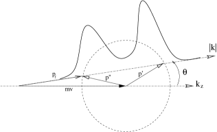
Figure 2: Kinematics of the breakup reaction. The solid curve represents the Coulomb energy distribution for a given small $\theta$.

On the other hand, in the nuclear breakup, Fig.(1a), the neutron average momentum in the projectile reference frame is $k_{z}\approx 0$, corresponding to the maximum of the initial momentum distribution and of the breakup probability. Then the energy distribution has just one peak at all angles, close to the incident energy (and momentum) per particle.

Double peaked longitudinal distributions are typical of reactions in which the mechanism of breakup involves an effective repulsive force between the fragments. For example in heavy-ion fragmentation reactions the so called Coulomb rings are observed [71]. This happens because the reaction goes through a kind of inelastic excitation in the projectile which then decays in flight. Therefore it is suggested that exclusive measurements of longitudinal distributions with the neutron in coincidence with the core, for fixed, small, angles $\theta$ could help distinguishing different reaction mechanisms. This could be very useful in the case of two-neutron halo breakup in which the second neutron decays in flight [29, 30, 31] from a resonant state and therefore with a mechanism different from the nuclear breakup which is responsible for the decay of the first neutron.

Figure 3: Neutron energy distributions following breakup of ¹¹Be at 41A.MeV for several targets (⁹Be, ⁴⁸Ti, ¹⁹⁷Au). Nuclear breakup distributions are represented by the dot-dashed line, Coulomb by the long dashed line, the Coulomb-nuclear coupling term by the dotted line, their coherent sum by the solid line. The dotted line with crosses is the nuclear plus the perturbative Coulomb incoherent sum.

We show in Figs.(3) the neutron final energy spectra for Coulomb and for nuclear breakup for the reactions ${}^{9}Be(^{11}Be,^{10}Be+n)^{9}Be$, ${}^{48}Ti(^{11}Be,^{10}Be+n)^{48}Ti$, ${}^{197}Au(^{11}Be,^{10}Be+n)^{197}Au$ at $E_{inc}$=41A.MeV [25] in the target reference frame. We have used the same low energy cutoff (27MeV) as in the experiment. We see that the nuclear breakup (dot-dashed line) is dominant for the ⁹Be target, for the ⁴⁸Ti target Coulomb (long dashed line) and nuclear give similar contributions, and for ¹⁹⁷Au, Coulomb breakup becomes dominant. The Coulomb-nuclear coupling term (dotted line) increases with the target mass and for ¹⁹⁷Au is of the same order as the pure nuclear term. From these results, we would expect big interferences between Coulomb and nuclear processes for ⁴⁸Ti and ¹⁹⁷Au. In fact the solid line which represents the coherent sum of the three processes is rather different from the dotted line with crosses, which is the incoherent sum of nuclear and perturbative Coulomb breakup.

Finally in Fig.(4a) we show the neutron energy spectrum in the projectile reference frame together with the data from [4] for Coulomb breakup on ${}^{208}Pb$ at $72$A.MeV. The same spectrum is also given in the target reference frame in Fig.(4b). Notation is the same as in Fig.(1). In this case as in the case of the Au target discussed before the contribution of the Coulomb-nuclear coupling term is very close to that of the pure nuclear term. Our results agree well with the experimental spectrum. We used the known spectroscopic factor $C^{2}S=0.77$ [72] for the s-initial state in ¹¹Be. The integrated Coulomb cross section is 1.70b to be compared with the experimental value of 1.8$\pm$ 0.4b. This is to show that our treatment of the Coulomb breakup by perturbation theory is accurate within the experimental error bars for the description of the shape and absolute magnitude of Coulomb breakup. It has been suggested [11, 12, 19, 20, 21] that a treatment beyond perturbation theory could be more accurate in same cases. Proton breakup, in particular at lower energies than those discussed here, is one of such cases. On the other hand methods that have studied consistently neutron breakup [1, 10] in first order or higher order, within the same model, have found negligible differences. Non perturbative treatments are also expected to be more accurate in the case of smaller neutron separation energies and lower beam energies [20] than those discussed here. The spectrum of Fig.(4) has been calculated and discussed in a number of theoretical works [10, 14, 15] which all use different non-perturbative methods but whose results are all consistent with each other and with our results, within the experimental error bars.

Figure 4: Neutron energy distributions following breakup of ¹¹Be on ²⁰⁸Pb at 72A.MeV in the projectile frame (a), and in the target frame (b). The notation is the same as in Fig.(1). Experimental points are from Nakamura [4].

4.2 Interference effects in the neutron angular distributions

Figure 5: Neutron angular distributions following breakup of ¹¹Be at 41A.MeV for several targets (⁹Be, ⁴⁸Ti, ¹⁹⁷Au). In the bottom figures the nuclear distribution is represented by the solid line, Coulomb by the long dashed line, and the Coulomb-nuclear term by the dotted line. In the top figures the coherent sum of the nuclear, Coulomb and Coulomb-nuclear terms by the solid line, the nuclear plus the perturbative Coulomb incoherent sum by the dashed line. Experimental points are from Anne [25].

Fig.(5) contains the data from the exclusive experiment of Ref. [25] in which the neutron angular distribution following the breakup from ¹¹Be was measured in coincidence with the ¹⁰Be ejectile. Three different targets were used to check on the relative importance of the nuclear and Coulomb breakup mechanisms. In the bottom part of the figure the solid line is the nuclear breakup cross section, the long dashed line is the Coulomb breakup while the dotted line is the Coulomb-nuclear coupling term. In the top part of the figure we show the experimental data together with the coherent sum of the three contributions (solid line). The dashed line is the nuclear plus the perturbative Coulomb incoherent sum. It is important to notice that the large angle scattering is due mainly to the nuclear breakup and it is sensitive to the neutron-target optical potential used. About two thirds of the total amount of nuclear breakup is due to large angle scattering. Therefore new measurements of neutron angular distributions, including large angle scattering data would greatly help in settling the question of the relative importance of nuclear and Coulomb breakup for heavy targets. On the other hand spectra of the type shown in Fig.(4a) correspond to small angle scattering only (typically $\theta<15$deg) where the nuclear is very small and therefore fitting them is not too significative for the understanding of the relative importance of the two reaction mechanisms.

Figure 6: Neutron angular distribution as in Fig.5, but 0$<\phi<$30 degrees for several targets (⁹Be, ⁴⁸Ti, ¹⁹⁷Au). The results in the top figures are integrated over the core target impact parameter d. The bottom figures are results at a fixed impact parameter $d=R_{s}$. The solid line represents the coherent sum of nuclear, Coulomb and Coulomb-nuclear terms. Their incoherent sum by the dashed line.

The theoretical results for the neutron angular distributions were summed over the neutron energy spectrum and averaged over its out-of-plane angle $\phi$ because this is what is contained in the experimental data. The peak values of the cross section show clearly an increase with the target due to the Coulomb breakup. From the comparison of the coherent and incoherent sums it is clear that coupling and interference effects are more important at the angles where nuclear and Coulomb terms are closer in magnitude, which happens at small $\theta$ for the ⁹Be target and around 20-30deg for the other two targets.

We have seen that the effects due to the interference are partially washed out by the average over $\phi$. On the other hand we have identified the reason of the lost of coherence at large $\theta$ in the integration of the probabilities over the core-target impact parameter d as contained in Eq.(31). To clarify these points we show in Fig. (6) similar calculations for the same targets as before but this time we have chosen to restrict the $\phi$ integration to the range $0\div 30$deg. In the top part the integral over the core-target impact parameter has been performed. In the bottom part of the figure the calculations have been performed integrating one fermi out of the strong absorption radius $R_{s}$. The results of these figures are however still summed over the neutron energy spectrum.

Figure 7: Cosinus of the Coulomb-nuclear phase as a function of the impact parameter for several $\theta$ angle and $\varepsilon_{f}=41MeV$ (fixed $k_{z}$, $k_{y}=0$, $k_{\perp}=k_{x}$). The solid line stands for $\theta=6$ degrees, the dashed line for $\theta=12$ degrees and the dot-dashed line for $\theta=18$ degrees. The target is ¹⁹⁷Au.

The solid lines are the results for the cross section obtained by summing coherently the nuclear and Coulomb and Coulomb-nuclear amplitudes while the dashed line is again the incoherent sum of the nuclear plus the perturbative Coulomb. From the bottom figure it is clear that the interferences change sign as a function of $\theta$.

Eqs.(16) and (22) show that the important contributions to the integral for the perturbative Coulomb amplitude come from the projectile region while integral (3.1) for the nuclear amplitude is weighted towards the target. As a consequence the Coulomb-nuclear phase difference has a dependence on the projectile-target impact parameter. The cosine of the relative Coulomb-nuclear phase as a function of $d$ is shown in Fig.(7) for a set of neutron emission angles. The neutron is emitted in the plane defined by the impact parameter and the incident beam direction. The cosine of the relative phase has a regular oscillatory behavior and the period of the oscillations decreases with increasing $\theta$. The oscillations reduce the magnitude of the Coulomb-nuclear interference. They also influence its sign as indicated by the integrated cross sections in Table 2.

Table 2: Integrated ($\theta=0\div 60$deg) breakup cross sections in barn. Incident energies in A.MeV.

Target	Einc	Coul-Nucl	Nuclear	Coulomb	Incoh. sum	Cohe. sum	%
9Be	30	0.6 10-3	0.200	0.011	0.212	0.222	5
	41	0.5 10-3	0.191	0.009	0.200	0.209	5
	120	0.4 10-4	0.044	0.004	0.048	0.050	5
48Ti	30	0.2 10-1	0.260	0.292	0.573	0.621	9
	41	0.2 10-1	0.252	0.229	0.496	0.531	8
	120	0.6 10-2	0.234	0.098	0.338	0.374	10
197Au	30	0.327	0.372	2.98	3.68	3.50	-5
	41	0.245	0.354	2.36	2.96	2.85	-4
	120	0.151	0.321	1.05	1.52	1.53	1
208Pb	72	0.148	0.346	1.70	2.19	2.17	-1

Finally we give in Table 2 the absolute cross sections for each individual term: the Coulomb-nuclear amplitude, the eikonal nuclear and Coulomb perturbative. Also their coherent and incoherent sums are shown, for the targets studied in this work. We have integrated in the experimental range $\theta=0\div 60$deg. In the calculations of this work we have used the strong absorption hypothesis Eq.(32) with the prescription $R_{s}=1.4(A_{P}^{1/3}+A_{T}^{1/3})fm$. Using the smooth absorption hypothesis [66] would reduce the absolute nuclear cross section but leave the energy and momentum distributions unchanged [8]. For example the total coherent cross sections on ⁹Be at the three given energies, with a smooth cut off are 0.221b, 0.200b and 0.042 b respectively. The same would happen using the new formalism proposed in [13]. The values without interference are very similar to those already obtained by some of us in [27]. We remind the reader that when the neutron is detected in coincidence with the core only the diffraction-type of nuclear breakup contributes. Cross section values are given at three incident energies $E_{inc}=30,41$ and $120$A.MeV and at $72$A.MeV for the ²⁰⁸Pb target. In the last column we give the percentage of interference effect. The effect of the interference on the angle integrated energy distribution is of the order of $4\div 10\%$ therefore small as already seen by other authors [2, 19, 32]. The interference is constructive for the ⁹Be and ⁴⁸Ti targets but destructive for the ¹⁹⁷Au and ²⁰⁸Pb targets. For the heavy targets it appears also that the interferences tend to vanish at high energy. Then from the analysis of the energy and angular distributions we conclude that the effect of the new Coulomb-nuclear coupling term and of the interferences is to give a slight increase with respect to the simple sum of the nuclear plus the Coulomb perturbative breakup. However from the analysis of the results for the total cross sections it appears that the total interference of the three terms can be destructive with respect to their sum for the heavy target. This is manly due to the imaginary part of the neutron target optical potential. The situation might be different in the case of the proton breakup studied in [17, 24, 21, 22] because the effective charge in the Coulomb potential Eq.(36) will be different from ours obtained for a neutron.

At this stage it is difficult to draw a general conclusion on the effects of the interference and of the Coulomb-nuclear coupling as they clearly depend on the target and on the incident energy and on the angular range covered by the experiment.

The results discussed in this paper are restricted to the 2s initial state in ¹¹Be. The Coulomb breakup from the d-component of the ground state gives a contribution two orders of magnitude smaller than the s-component and thus it has been neglected here. However the formulae given in the appendix hold for any initial angular momentum. Calculations for cases like the weakly bound carbon isotopes, where $l_{i}=2$ orbitals are important, will be presented elsewhere.

5 Conclusions

In this work we have derived an eikonal formalism leading to Eq.(11) to treat consistently the nuclear and Coulomb breakup to all orders in the interactions. This formula could be studied numerically. Here we have studied only the effect of the first order coupling and interference between the two processes. By taking first order terms in the Coulomb potential and the nuclear potential to all orders we have obtained a scheme in which the breakup amplitude is a sum of three terms. Two of them reduce to the well known forms of the nuclear breakup in the eikonal model and of the Coulomb breakup in first order perturbation theory. The third term, Eq.(24) which is derived here for the first time, depends on both the Coulomb and nuclear potentials and can be viewed as one of the lowest ”higher order coupling terms”. Within such a model numerical results show that interferences between nuclear and Coulomb breakup are present in halo nucleus reactions and in the data already existing. They are responsible for the peak at small angles in the angular distribution on the ⁹Be target and for the behavior at large $\theta$ in the case of heavier targets. They have not been seen so far more clearly in the data because of the averaging over the neutron out-of-the-reaction plane angle $\phi$ and the integration over the core-target impact parameter. However they would show up in neutron double differential angular distribution from halo breakup by making a selection on a small range of $\phi$ angles and detecting the core at fixed angles, provided it follows a Coulomb trajectory. In this case the reaction plane could be identified and a one by one correspondence between the core detection angle and the trajectory impact parameter could be applied.

The Coulomb-nuclear interference effects are small for the cases studied in the this paper. Interference terms do not have a definite sign in the angular distribution but they are overall constructive in the energy spectra and absolute cross sections at medium energies and for light to medium mass targets. For heavy targets the results presented here show an overall destructive interference which depends on the imaginary part of the neutron target optical potential and which tends to vanish increasing the beam energy. The effect of the new Coulomb-nuclear coupling term is rather small and negligible for light targets, while for heavy targets is of the same order as the pure nuclear term. This is evident in the energy distributions and in the small angle angular distributions. The comparison with the data and with other works is reassuring in so far as the neglect of higher order terms in the Coulomb amplitude is concerned. They scale as powers of the effective charge, that is as powers of $C=\beta_{1}Z_{P}Z_{T}e^{2}/\hbar v$ and $\beta_{1}$ is small ($\beta_{1}=0.1)$ for the ¹¹Be projectile. Higher order terms will be very small for light targets but could become more important for heavy targets. They have not been studied here but they can be evaluated within the adiabatic approximation Eq.(27).

Thus it appears that the so-called Coulomb experiments would need a more accurate theoretical analysis than performed so far. Also we think that it would be very important to measure more neutron angular distributions, like the ones [25] discussed in this paper. They are a beautiful tool to identify the reaction mechanism and to test the theoretical methods. Therefore we suggest that in more exclusive kind of experiments it should be possible to see better the effects discussed in this work. It will be necessary to have more intense radioactive beams giving also a better statistics and to use neutron position sensitive detectors over a wide angular range. New facilities of the type being planned in Europe (EURISOL) and USA (RIA) are therefore most welcome.

Acknowledgments

We wish to thank E. Piasecki for drawing Ref.[71] to our attention and for suggesting Fig.(2).

Appendix A Details of the Coulomb and Coulomb-nuclear amplitudes.

The Coulomb contribution to the effective interaction is

$$V_{eff}(\mathbf{r},t)=+{\beta}_{1}Z_{P}Z_{T}e^{2}\frac{xd+zvt}{\left(d^{2}+\left(vt\right)^{2}\right)^{3/2}}$$ (36)

We need to evaluate several integrals. The first is the Fourier transform

$$\chi_{eff}\left(\mathbf{r},\omega\right)=\frac{1}{\hbar}\int_{-\infty}^{\infty}dte^{i\omega t}V_{eff}\left(\mathbf{r},t\right)$$ (37)

By making a change of variables $s=vt/d$ the first integral becomes

$$\chi_{eff}\left(\mathbf{r},\omega\right) = \frac{C}{d}\int_{-\infty}^{\infty}dse^{i\varpi s}\frac{x+zs}{\left(1+s^{2}\right)^{3/2}}$$ (38)

$$= 2\frac{C}{d}\left(x\varpi K_{1}\left(\varpi\right)+iz\varpi K_{0}\left(\varpi\right)\right)$$

where

$$\varpi=\frac{\omega d}{v}=\frac{(\varepsilon_{\mathbf{k}}-\varepsilon_{0})d}{\hbar v}.$$ (39)

and the constant $C={\beta}_{1}Z_{P}Z_{T}e^{2}/\hbar v$ is a dimensionless interaction strength. The functions$K_{0}$ and $K_{1}$ are modified Bessel functions and can be defined by the integrals

$$\varpi K_{1}\left(\varpi\right) = {\frac{1}{2}}\int_{-\infty}^{\infty}\frac{\cos\left(\varpi t\right)dt}{\left(1+t^{2}\right)^{3/2}}$$ (40)

$$\varpi K_{0}\left(\varpi\right) = {\frac{1}{2}}\int_{-\infty}^{\infty}\frac{t\sin\left(\varpi t\right)dt}{\left(1+t^{2}\right)^{3/2}}$$ (41)

Substituting eq.(38) into eq.(22) yields the perturbation amplitude

$$g_{r}^{pert}\left(\mathbf{k,}\mathbf{d}\right) = -i\frac{2C}{d}\int d^{3}\mathbf{r}e^{-i\mathbf{k.r}}\left(x\varpi K_{1}\left(\varpi\right)+iz\varpi K_{0}\left(\varpi\right)\right)\phi_{lm}\left(\mathbf{r}\right)$$ (42)

$$= 2\frac{{C}}{d}\left(\varpi K_{1}\left(\varpi\right)\frac{d}{dk_{x}}+i\varpi K_{0}\left(\varpi\right)\frac{d}{dk_{z}}\right)\tilde{\phi}_{lm}\left(\mathbf{k}\right).$$

The constant $C={\beta}_{1}Z_{P}Z_{T}e^{2}/\hbar v$ is a dimensionless interaction strength and $\varpi$ is the adiabaticity parameter. The functions $K_{0}$ and $K_{1}$ are modified Bessel functions and $\tilde{\phi}_{lm}\left(\mathbf{k}\right)$ is the Fourier transform of $\phi_{lm}\left(\mathbf{r}\right)$. First order perturbation theory in $\ V_{eff}$ should be a good approximation if $CR_{p}/d<1/2$ where $R_{p}$ is the radius of the halo nucleus. Numerical values for the modified Bessel functions show that the adiabatic or ’frozen halo’ approximation should be satisfactory if $\varpi<0.2$.  Eq.(42) is the standard dipole expression for Coulomb breakup.

The function

$$B\left(x,z,\varpi\right)=\frac{i}{\hbar}\left[\int_{-\infty}^{0}dte^{i\omega t}V_{eff}\left(\mathbf{r},t\right)+\int_{0}^{\infty}dtV_{eff}\left(\mathbf{r},t\right)\right]$$ (43)

involves two integrals. The first is

$$\frac{1}{\hbar}\int_{0}^{\infty}dtV_{eff}\left(\mathbf{r},t\right)=\frac{C}{d}\left(x+z\right)$$ (44)

The other is a one-sided Fourier transform

$$\frac{1}{\hbar}\int_{-\infty}^{0}dte^{i\omega t}V_{eff}\left(\mathbf{r},t\right)=\frac{1}{\hbar}\int_{0}^{\infty}dte^{-i\omega t}V_{eff}\left(\mathbf{r},-t\right)$$ (45)

It can be expressed in terms of $\varpi K_{0}\left(\varpi\right),\varpi K_{1}\left(\varpi\right)$ and two new integrals

$$\varpi\bar{K}_{1}\left(\varpi\right) = \int_{0}^{\infty}\frac{\sin\left(\varpi t\right)dt}{\left(1+t^{2}\right)^{3/2}}$$ (46)

$$\varpi\bar{K}_{0}\left(\varpi\right) = \int_{0}^{\infty}\frac{t\cos\left(\varpi t\right)dt}{\left(1+t^{2}\right)^{3/2}}$$ (47)

Putting everything together

$$B\left(x,z,\varpi\right)=i\frac{C}{d}\left(x(\varpi K_{1}\left(\varpi\right)+1-i\varpi\bar{K}_{1}\left(\varpi\right))-z\left(\varpi\bar{K}_{0}\left(\varpi\right)-1-i\varpi K_{0}\left(\varpi\right)\right)\right)$$ (48)

Appendix B Initial states with general angular momenta.

B.1 The Coulomb breakup amplitude.

If the initial state wave function is approximated by its asymptotic form which is an Hankel function [73]

$$\phi_{lm}(r)=-i^{l}C_{i}\gamma_{0}h_{l}^{(1)}(i\gamma_{0}r)Y_{lm}(\theta,\phi),\,\,\,\gamma_{0}r>>1,$$ (49)

where $C_{i}$ is the asymptotic normalization constant [70] and $\gamma_{0}=\sqrt{-2m\varepsilon_{0}}/\hbar$, then the general form of the initial state momentum distribution is given by the Fourier transform of Eq.(49)

$$\widetilde{\phi}_{lm}({\bf k_{\perp}},k_{z})=4\pi C_{1}{{k}^{l}\over\gamma_{0}^{l}(k_{\perp}^{2}+k_{z}^{2}+\gamma_{0}^{2})}Y_{l,m}(\hat{k})$$ (50)

where ${\bf{k}}\equiv(k_{x},k_{y},k_{z})$ is a real vector.

In nuclear breakup reactions the use of the asymptotic part of the initial bound state wave function is justified because of the short range nature of the nuclear interaction which gives breakup form factors in Eq.(3.1) localized in the overlap region between the two interacting nuclei. The amplitude for Coulomb breakup is expressed in terms of the Fourier transform of the bound state wave function in Eq.(42). This Fourier transform is well approximated by the Fourier transform Eq.(50) of the corresponding Hankel function provided that $\gamma_{0}R<<1$ and $kR<<1$ where $R$ is the nuclear radius. These conditions are often satisfied in the Coulomb breakup of a halo nucleus. We have checked this for ¹¹Be using wave functions calculated in a square-well potential and have shown that for $|\varepsilon_{0}|\leq 1$MeV and up to $l=2$ the contribution of the internal part of the wave function to the full Fourier transform can be neglected.

We want to evaluate $2\pi<\sum_{m}|A_{lm}^{Coul}|^{2}>_{\varphi}$ where $<>_{\varphi}$ stands for the average over the $\varphi$ angle of ${\bf k}_{f}$. Some definitions for the neutron momenta are: ${\bf k}_{f}=(k_{x},k_{y},k_{f_{z}})$ is the neutron final momentum in the target reference frame, while ${\bf k}=(k_{x},k_{y},k_{z})$ is in the projectile reference frame and $k_{z}=k_{f_{z}}-m_{n}v/\hbar$, $k_{\perp}^{2}=k_{x}^{2}+k_{y}^{2}$.

We define

$${\cal A}_{lm}^{Coul}=\left(K_{1}(\bar{\omega})\frac{\partial}{\partial k_{x}}+iK_{0}(\bar{\omega})\frac{\partial}{\partial k_{z}}\right)F_{lm}({\bf k})$$ (51)

where $K_{1}$ and $K_{2}$ are modified Bessel functions and

$$F_{lm}(\hat{k}) = f_{l}(k)Y_{lm}(\hat{\bf k})$$ (52)

$$f_{l}(k) = \frac{k^{l}}{\gamma_{0}^{l}(\gamma_{0}^{2}+k_{\perp}^{2}+k_{z}^{2})}$$ (53)

with $\gamma_{0}=\sqrt{-2m\epsilon_{0}}/h$. Then

$${\cal B}_{l}=\sum_{m}F_{lm}^{*}({k}^{\prime})F_{lm}({k})=\frac{2l+1}{4\pi}f(k^{\prime})f(k)P_{l}(\cos\Theta)$$ (54)

with $\cos\Theta={\bf k}.{\bf k}^{\prime}/k^{\prime}k$.

We calculate the derivatives like $\partial^{2}{\cal B}_{l}/\partial k^{\prime}_{x}\partial k_{x}$ and finally put ${\bf k}^{\prime}={\bf k}$. Note that $\partial/\partial k^{\prime}_{x}P_{l}(\cos\theta)|_{{\bf k}={\bf k}^{\prime}}=0$.

Using the above results in Eq.(51) and averaging over $\varphi$

$$2\pi<\sum_{m}|{\cal A}_{lm}^{Coul}|^{2}>_{\varphi} = \frac{2l+1}{2(k_{\perp}^{2}+k_{z}^{2})^{2}}\left(K_{1}^{2}(\bar{\omega})\left[f^{\prime 2}k^{2}k_{\perp}^{2}/2+P^{\prime}_{l}(1)f^{2}(k_{z}^{2}+k_{\perp}/2)\right]\right.$$ (55)

$$+ \left.K_{0}^{2}(\bar{\omega})\left[f^{\prime 2}k^{2}k_{z}^{2}/2+P^{\prime}_{l}(1)f^{2}k_{\perp}^{2}\right]\right)$$

After simplifications, the final result is

$$2\pi<\sum_{m}|{\cal A}_{lm}^{Coul}|^{2}>_{\varphi} = \frac{2l+1}{2}\left(K_{1}^{2}\,[{\cal U}_{l}+\frac{1}{2}k_{\perp}^{2}{\cal V}_{l}]+K_{0}^{2}\,[{\cal U}_{l}+k_{z}^{2}{\cal V}_{l}]\right)$$ (56)

with

$${\cal U}_{l}(k) = \frac{l(l+1)}{2}\frac{k^{2l-2}}{\gamma^{2l}(\gamma_{0}^{2}+k^{2})^{2}}$$ (57)

$${\cal V}_{l}(k) = \frac{k^{2l-4}}{\gamma_{0}^{2l}(\gamma_{0}^{2}+k^{2})^{4}}\left[\frac{l(l-1)}{2}(\gamma_{0}^{2}+k^{2})^{2}-4lk^{2}(\gamma_{0}^{2}+k^{2})+4k^{4}\right]$$ (58)

B.2 The Coulomb cross section.

We give in the following the analytical formulae for the cross section due to Coulomb breakup only obtained using Eqs.(31,32,42). In the integral Eq.(31) over the impact parameter d we change variable of integration from d to $\bar{\omega}$ given in Eq.(39). Furthermore to compare to experimental angular distributions we average over the angle $\phi$. The expressions for the double differential cross section, in the case of an initial s and p state are

$${d^{2}\sigma_{Coul}\over d\varepsilon_{f}d\Omega}={mk_{f}\over\hbar^{2}}\left({CC_{1}\bar{\bar{\omega}}}\right)^{2}{2\over\pi(k_{\perp}^{2}+k_{z}^{2}+\gamma_{0}^{2})^{4}}\left[{\cal A}(K_{1}^{2}-K_{0}^{2})+{\cal B}K_{0}K_{1}\right]$$ (59)

where

$${\cal A}=4\left(k_{z}^{2}-{k_{\perp}^{2}\over 2})\right)$$ (60)

and

$${\cal B}=4{k_{\perp}^{2}\over\bar{\bar{\omega}}}$$ (61)

in the case of an s-initial state, while for a p-initial state we get

$${\cal A}={1\over\gamma_{0}^{2}}\left(k_{\perp}^{4}+(k_{z}^{2}+\gamma_{0}^{2})^{2}+{k_{\perp}^{2}\over 2(k_{\perp}^{2}+\gamma_{0}^{2})}(k_{\perp}^{2}+\gamma_{0}^{2}-k_{z}^{2})^{2}+4k_{z}^{2}(2k_{\perp}^{2}+\gamma_{0}^{2})\right)$$ (62)

$${\cal B}=-{1\over\gamma_{0}^{2}}\left({2\over\bar{\bar{\omega}}}\left(k_{\perp}^{4}+(k_{z}^{2}+\gamma_{0}^{2})^{2}+{k_{\perp}^{2}\over 2(k_{\perp}^{2}+\gamma_{0}^{2})}(k_{\perp}^{2}+\gamma_{0}^{2}-k_{z}^{2})^{2}\right)\right)$$ (63)

$\bar{\bar{\omega}}={\bar{\omega}}(d=R_{s})$ is the argument of the modified Bessel functions in Eq.(59).

References

- [1] S. Typel and G. Baur, Phys. Rev. C 64, 024601 (2001).
- [2] S. Typel and R. Shyam, Phys. Rev. C 64, 024605 (2001).
- [3] H. Esbensen, Proceedings of the 4th course of the International School in Heavy Ion Physics, Erice, May 1997, Ed. R. A. Broglia end P. G. Hansen, World Scientific.
- [4] T. Nakamura, Phys. Lett. B331, 296 (1994).
- [5] T. Nakamura et al., Phys. Rev. Lett. 83, 1112 (1999).
- [6] V. Maddalena et al., Phys. Rev. C63, 024613 (2001) and references therein.
- [7] V. Maddalena and R. Shyam, Phys. Rev. C63 , 051601 (2001).
- [8] A. Bonaccorso, Phys. Rev. C60, 054604 (1999), and references therein.
- [9] H. Esbensen, and G. F. Bertsch, Phys. Rev. C 64 (2001) 014608.
- [10] H. Esbensen, G. Bertsch and C.A. Bertulani, Nucl. Phys. A581 107 (1995).
- [11] T. Kido, K. Yabana and Y. Suzuki Phys. Rev. C53 2296 (1996).
- [12] V. S. Melezhik and D. Baye, Phys. Rev. C59 3232 (1999).
- [13] A. Bonaccorso and G. F. Bertsch, Phys. Rev. C63, 044604 (2001).
- [14] P. Banerjee, I. J. Thompson and J. A. Tostevin, Phys. Rev. C58 1042 (1998).
- [15] R. Chatterjee, P. Banerjee, R. Shyam, Nucl. Phys. A675 477 (2000).
- [16] P. Banerjee and R. Shyam, Phys. Rev. C61 047301 (2000).
- [17] C. H. Dasso, S. M. Lenzi and A. Vitturi, Nucl. Phys. A639, 635 (1998).
- [18] C. H. Dasso, S. M. Lenzi and A. Vitturi, Phys. Rev. C59 539 (1999).
- [19] M. Fallot, J. A. Scarpaci, D. Lacroix, Ph. Chomaz and J. Margueron, Nucl. Phys. A (2001) in press.
- [20] J. A. Tostevin, S. Rugmai and R. C. Jonhson, Phys. Rev. C57 3225 (1998). J.A. Tostevin, ”Fission and Properties of Neutron-rich Nuclei”, Proceedings of the Second International Conference (St Andrews, Scotland, 28 June - 3 July 1999) ed J H Hamilton, W R Phillips and H K Carter, World Scientific (Singapore), March 2000, pp 429-438.
- [21] F. M. Nunes and I. J. Thompson, Phys. Rev. C59, 2652 (1999).
- [22] H. Esbensen and K. Hencken, Phys. Rev. C61, 054606 (2000).
- [23] H. Esbensen, and G. F. Bertsch Nucl. Phys. A600 37 (1996) .
- [24] R. Shyam and I. J. Thompson, Phys. Rev. C59, 2645 (1999).
- [25] R. Anne et al., Nucl.Phys. A575, 125 (1994).
- [26] A. Bonaccorso and D. M. Brink, Phys. Rev. C57, R22 (1998).
- [27] A. Bonaccorso and D. M. Brink, Phys. Rev. C58, 2864 (1998).
- [28] F. Barranco and P. G. Hansen, Eur. Phys. J. A7 479 (2000).
- [29] F. Barranco, E. Vigezzi and R. A. Broglia, Phys.Lett. B319, 387 (1993).
- [30] L. V. Chulkov et al, Phys. Rev. Lett. 79 201 (1997). L. V. Chulkov and G. Schrieder, Z. Phys. A359 231 (1997). D. Aleksandrov et al., Nucl. Phys. A669 51 (2000) and references therein.
- [31] F. M. Marqués et al., Phys. Rev. C 64, 061301 (2001).
- [32] C. A. Bertulani and G. Baur, Nucl. Phys. A480 615 (1988).
- [33] C. A. Bertulani and K. W. Mc Voy, Phys. Rev. C46, 2638 (1992).
- [34] Y. Ogawa, K. Yabana, and Y. Suzuki, Nucl. Phys.A543 (1992) 722.
- [35] H. Sagawa and N. Takigawa, Phys. Rev. C50, 985 (1994) .
- [36] A. A. Korsheninnikov and T. Kobayashi , Nucl.Phys. A 576, (1994) 97.
- [37] K. Hencken, G. Bertsch and H. Esbensen, Phys.Rev. C54, 3043, (1996).
- [38] T. Kobayashi et al, Phys. Lett. B232 (1989) 51
- [39] T. Kobayashi et al, Nucl. Phys. A538 (1992) 343c
- [40] K. Ieki et al, Phys. Rev. Lett. 70 (1993) 730
- [41] D. Sackett et al, Phys. Rev. C48 (1993) 118
- [42] S. Schimoura et al, Phys. Lett. B348 (1995) 29
- [43] T. Kobayashi, Nucl. Phys. A553 (1993) 465c
- [44] A. A. Korsheninnikov et al, Phys. Rev. C53 (1996) R537
- [45] P. G. Hansen and B. Jonson, Europhys.Lett.4 (1887) 409
- [46] G. Bertsch and J. Foxwell, Phys. Rev. C41 (1990) 1300
- [47] G. Bertsch and H. Esbensen, Nucl. Phys. A542 (1992) 310
- [48] K. Ikeda, Nucl. Phys. A538 (1992) 355c
- [49] Y. A. Lurie, A. M. Shirokov and Y. F. Smirnov, Conference ”Halo-94”-Copenhagen (1994)
- [50] C. A. Bertulani, G. Baur and M. S. Hussein, Nucl. Phys. A526 (1991)751
- [51] C. A. Bertulani and L. F. Canto, Nucl. Phys. A539 (1992) 163
- [52] H. Sagawa, N. Takigawa and N. Van Giai, Nucl. Phys. A543 (1992) 575
- [53] F. Catara, C.H. Dasso and A. Vitturi, Nucl. Phys. A602 (1996) 181.
- [54] A. Bonaccorso and N. Vinh Mau, Nucl. Phys. A 615 (1997) 245.
- [55] A. I. Amelin et al, Sov.J. Nucl. Phys. 52 (1990) 782.
- [56] M. Zinser et al, Phys. Rev. Lett. 75 (1995) 1719.
- [57] M. Bernas, J. C. Peng and N. Stein, Phys. Lett. B116 (1982) 7.
- [58] H. Sagawa et al, Z. Phys. A351 (1995) 385
- [59] G. Bertsch, H. Esbensen and A. Sustich, Phys. Rev. C42 (1990) 758.
- [60] H. Esbensen, Phys. Rev. C44 (1991) 440.
- [61] A. Sustich, Z. Phys. A342 (1992) 31.
- [62] H. Riisager et al, Nucl. Phys. A540(1992)365.
- [63] R. Shyam and P. Danielewicz, Phys. Rev. C63 054608 (2001).
- [64] H. Okamura et al., Phys. Lett. B325 308 (1994).
- [65] A. Winther and K. Adler, Nucl. Phys. A319 518 (1979).
- [66] A. Bonaccorso, D. M. Brink and L. Lo Monaco, J. Phys. G 13, (1987) 1407.
- [67] A. Bonaccorso and D. M. Brink, Phys. Rev. C44, 1559 (1991).
- [68] A. Bonaccorso and D. M. Brink, Phys. Rev. C38, 1776 (1988).
- [69] A. Bonaccorso and D. M. Brink, Phys. Rev. C44 (1991) 1559.
- [70] A. Bonaccorso, G. Piccolo and D. M. Brink, Nucl.Phys. A441, 555 (1985).
- [71] R. J. Charity et al., Nucl. Phys. A476, 516 (1988), Nucl. Phys. A483, 371 (1988).
- [72] F. Ajzenberg-Selove, Nucl. Phys. A506 1 (1990).
- [73] L. I. Schiff, Quantum Mechanics, Mc Graw-Hill Kogasha Ltd , Tokyo 1968, Pag. 44.