Coherent Compton scattering on light nuclei in the $\Delta$-resonance region

Abstract

Coherent Compton scattering on light nuclei in the $\Delta$ resonance region is studied in the impulse approximation and is shown to be a sensitive probe of the in-medium properties of the $\Delta$ resonance. The elementary amplitude on a single nucleon is calculated from the unitary K-matrix approach developed previously. Modifications of the properties of the $\Delta$ resonance due to the nuclear medium are accounted for through the self-energy operator of the $\Delta$, calculated from the one-pion loop. The dominant medium effects such as the Pauli blocking, mean-field modification of the nucleon and $\Delta$ masses, and particle-hole excitations in the pion propagator are consistently included in nuclear matter.

2001 PACS numbers: 25.20.Dc, 13.60.Fz

I Introduction

Coherent Compton scattering on nuclei in the region of the $\Delta$ resonance is of considerable interest. The reaction allows one to study the propagation and decay of the $\Delta$ in the nuclear medium. In particular the shift of the pole position and a change of the width of the $\Delta$ peak, reflect sensitively in the cross section and polarization observables.

For a comprehensive review on Compton scattering we refer to the recent reference [1]. Here we only mention several models relevant for the present study. The so-called ”schematic and extended” models [2, 3] made use of the optical theorem and dispersion relations to relate the Compton-scattering amplitude with the total photoabsorption cross section. Important contributions to the amplitude, such as nuclear kinetic and meson seagull terms, and $\Delta$ excitation, were added explicitly [3]. The data for Compton scattering were described quite well at forward scattering angles.

Compton scattering was extensively studied in the $\Delta$-hole model [3, 4, 5] which was originally developed by Koch, Moniz and Ohtsuka in [6, 7]. The $\Delta$ excitation is included through the $M1$ transition, the background is represented by the Kroll-Ruderman part of the virtual-pion photoproduction amplitude, while in Refs. [3, 5] the proton Thomson term (with $E1$ multipolarity) is also added.

The starting point of the present model is the full Compton-scattering amplitude $T_{N}$ on a free nucleon that includes all dominant mechanisms at energies up to, at least, the $\Delta$ resonance. This amplitude has been obtained in the unitary K-matrix approach, similar to the calculations presented in refs. [8, 9] for pion-nucleon scattering, pion photoproduction and Compton scattering on the proton. Parameters of the model are fixed from a detailed fit to observables for the above elementary reactions. The Thomson limit dictated by the low-energy theorem on the nucleon and the Kroll-Ruderman term of the photoproduction amplitude are automatically included.

Medium effects are taken into account via the self-energy of the $\Delta$, while the self-energy is calculated from the pion-loop mechanism embedded in nuclear matter, as described in detail in sect.II. In particular, Pauli blocking effects, mean-field modifications of the nucleon and $\Delta$ masses, and particle-hole contributions to the pion propagator are consistently calculated. Thus we avoid arbitrariness associated with introducing a parameterized self-energy.

The amplitude on a nucleus is calculated in the impulse approximation. A formfactor is introduced to account for finite size effects. The specific density dependence of the medium effects is accounted for through a local density approximation. Fermi-motion is treated in the so-called factorization approximation, in which the elementary Compton-scattering amplitude is calculated on a nucleon with an effective momentum [10, 11, 12, 13]. The latter is taken in such a way that the energy-momentum conservation for the $\gamma\,N$ scattering holds, thus ensuring gauge invariance at the one-body level.

Differential cross sections and photon asymmetries are calculated for light nuclei (⁴He and ¹²C) in the energy region 150 – 250 MeV.

The structure of the paper is as follows. In sect.II we describe the calculation of medium effects in the $\Delta$ propagator. Sect.III presents the basic formalism for calculating the Compton-scattering amplitude on nuclei in the impulse approximation. Results for the cross section and photon asymmetry are presented in sect.IV. Conclusions and prospects are further outlined. In Appendix A formulas for the pion self-energy are collected. Details of the kinematics involved in the reaction on a nucleus are contained in Appendix B.

II Medium modifications of the $\Delta$ resonance

The properties of the $\Delta$ in the nuclear medium are calculated in a relativistic framework for symmetrical nuclear matter, along the lines of Refs. [14, 15, 16]. The medium modifications, which are expressed through the dressing of the $\Delta$ propagator, are investigated using different levels of approximation. The imaginary part of the $\Delta$ self-energy (or the $\Delta$ decay width) is calculated in different models for the nuclear medium. Dispersion relations are used to determine the real part (mass modification) of the $\Delta$ self-energy.

In a first subsection the Rarita-Schwinger formalism is introduced to describe the $\Delta$ resonance. The next three subsections deal with the $\Delta$ decay width. In a first step the nuclear medium is presented as a non-interacting Fermi-sea of nucleons leading to the calculation of the Pauli-corrected decay width and the spreading width. Subsequently mean-field effects are included within the $\sigma\omega-$model of Walecka [17]. Throughout, the conventions of Bjorken and Drell [18] are used, and all expressions are derived in the nuclear matter rest frame.

A Formalism for the $\Delta$ self-energy

The free $\Delta$ propagator in the Rarita-Schwinger formalism has the following form [19]:

$$G_{\Delta}^{0}(p_{\Delta})^{\mu\nu} = \frac{1}{\hbox to0.0pt{/\hss}p_{\Delta}-M_{\Delta}+i\epsilon}\,\Biggl{[}\,g^{\mu\nu}-\frac{1}{3}\gamma^{\mu}\gamma^{\nu}-\frac{2p_{\Delta}^{\mu}p_{\Delta}^{\nu}}{3M_{\Delta}^{2}}-\frac{\left(\gamma^{\mu}p_{\Delta}^{\nu}-\gamma^{\nu}p_{\Delta}^{\mu}\right)}{3M_{\Delta}}\,\Biggr{]}$$ (1)

with the mass $M_{\Delta}=1232$ MeV and $p_{\Delta}=(p_{\Delta}^{0},\,\vec{p}_{\Delta})$. The invariant mass of the $\Delta$ resonance will be denoted by $W_{\Delta}=(p_{\Delta}^{2})^{1/2}$.

The propagator has to be dressed due to the interaction of the $\Delta$ with the nuclear medium. This is taken into account by introducing the self-energy in the equation for the inverse propagator

$$(G_{\Delta}^{-1})^{\mu\nu} = ((G^{0}_{\Delta})^{-1})^{\mu\nu}-\Sigma_{\Delta}^{\mu\nu}=(\hbox to0.0pt{/\hss}p_{\Delta}-M_{\Delta})\,({\cal P}^{3/2})^{\mu\nu}$$ (2)

$$- 2(\hbox to0.0pt{/\hss}p_{\Delta}-M_{\Delta})\,({\cal P}^{1/2}_{11})^{\mu\nu}+\sqrt{3}M_{\Delta}[\,({\cal{P}}^{1/2}_{12})^{\mu\nu}+({\cal P}^{1/2}_{21})^{\mu\nu}\,]-\Sigma_{\Delta}^{\mu\nu}\,,$$ (3)

where the inverse free propagator is written in terms of the projection operators on the spin-3/2 and spin-1/2 sectors [20] ($\,{\cal P}^{3/2},\,{\cal P}^{1/2}_{ij},\,ij=11,\,22,\,12,\,21\,$). In this paper we concentrate on the dominant spin-3/2 component of the $\Delta$ propagator, and therefore the self-energy is taken as

$$\Sigma_{\Delta}^{\mu\nu}=\Sigma_{\Delta}^{3/2}\;({\cal{P}}^{3/2})^{\mu\nu},$$ (4)

where we discarded terms proportional to the spin-1/2 projection operators. The spin-3/2 component of the self-energy has the structure

$$\Sigma_{\Delta}^{3/2}=C_{\Delta}(p_{\Delta})+D_{\Delta}(p_{\Delta})\,\hbox to0.0pt{/\hss}{p_{\Delta}}\,,$$ (5)

and the dressed propagator becomes

$$G_{\Delta}(p_{\Delta})^{\mu\nu} = \frac{1}{\hbox to0.0pt{/\hss}p_{\Delta}-M_{\Delta}-\Sigma_{\Delta}^{3/2}}\ ({\cal P}^{3/2})^{\mu\nu}$$ (6)

$$= [{\hbox to0.0pt{/\hss}p_{\Delta}}(1-ReD_{\Delta}(p_{\Delta}))-(M_{\Delta}+ReC_{\Delta}(p_{\Delta}))$$ (7)

$$- i(ImC_{\Delta}(p_{\Delta})+ImD_{\Delta}(p_{\Delta})\hbox to0.0pt{/\hss}{p_{\Delta}})]^{-1}\ ({\cal{P}}^{3/2})^{\mu\nu}.$$ (8)

Note that in vacuum $C_{\Delta}(p_{\Delta})$ and $D_{\Delta}(p_{\Delta})$ are functions of the invariant $W_{\Delta}$ only, while in the medium these functions acquire additional dependencies on the 3-momentum $|\vec{p}_{\Delta}|$ and the nuclear density $\rho$. We keep $p_{\Delta}$ as an argument in Eq. (5) for the general situation.

B Width of the $\Delta$ resonance and Pauli blocking

The imaginary part of the $\Delta$ self-energy is calculated from an effective interaction Lagrangian. We focus on the pion-nucleon decay channel in a nuclear environment. The $\pi N\Delta$ interaction Lagrangian is taken in the form [20, 21, 22]

$${\cal L}_{\pi N\Delta}=\frac{f_{\pi N\Delta}}{m_{\pi}}\ g^{\mu\nu}\overline{\Delta}_{\mu}\vec{T}^{\dagger}\Psi\ (\partial_{\nu}\vec{\pi})\ +\ H.c.\,,$$ (9)

where $\Psi$ ($\Delta_{\mu}$) is the nucleon ($\Delta$) field operator, $\vec{\pi}$ the pion field, and ${T}_{i}$ is the isospin $\frac{1}{2}\leftrightarrow\frac{3}{2}$ transition operator with the normalization condition ${T}_{i}{T}^{\dagger}_{j}=\delta_{ij}-\frac{1}{3}{\tau}_{i}{\tau}_{j}\,,\;\;\;(i,j=1,2,3)\,.$ In the above Lagrangian we dropped the off-shell coupling of the $\Delta$ described by the parameter $z_{\pi}$ [20, 21, 22], since it affects only the spin-1/2 components which are not considered in the present work.

The width of the resonance is defined by the imaginary part of the self-energy as

$$\Gamma_{\Delta}(p_{\Delta})=-2Im\,[\,C_{\Delta}(p_{\Delta})+W_{\Delta}D_{\Delta}(p_{\Delta})\,].$$ (10)

This can more formally be written as a trace

$$\Gamma_{\Delta}(p_{\Delta})=-2Im\,\left[\frac{1}{4}\,Tr\,\left(\,\Sigma_{\Delta}^{\mu\nu}\,({\cal P}^{3/2})_{\nu\mu}\,\frac{(\hbox to0.0pt{/\hss}{p}_{\Delta}+W_{\Delta})}{2W_{\Delta}}\,\right)\right]$$ (11)

The contribution to the self-energy for a $\Delta$ decaying into a nucleon and a pion is

$$-i\left(\Sigma_{\Delta}\right)_{\mu\nu}=\Big{(}\frac{f_{\pi N\Delta}}{m_{\pi}}\Big{)}^{2}\sum_{a=1,2,3}\int\frac{d^{4}k}{(2\pi)^{4}}q_{\mu}T^{\dagger}_{a}G_{N}(k)(-q_{\nu})T_{a}D_{\pi}(q),$$ (12)

where $q=p_{\Delta}-k$, and $G_{N}(k)$ and $D_{\pi}(q)$ are the nucleon and pion propagators, the structure of which depends on the model used for the nuclear medium. We will now discuss different approximations and their implications for the $\Delta$ decay width.

In vacuum the nucleon and pion propagators in (12) reduce to the free nucleon propagator

$$G_{N}^{0}(k)=\frac{1}{\hbox to0.0pt{/\hss}{k}-M_{N}+i\epsilon}=\frac{M_{N}}{E_{\vec{k}}}\left(\frac{\Lambda^{+}(\vec{k})}{k_{0}-E_{\vec{k}}+i\epsilon}-\frac{\Lambda^{-}(-\vec{k})}{k_{0}+E_{\vec{k}}-i\epsilon}\right)$$ (13)

and the free pion propagator

$$D_{\pi}^{0}(q)=\frac{1}{q^{2}-m_{\pi}^{2}+i\epsilon}\,,$$ (14)

where $E_{\vec{k}}=\sqrt{|\vec{k}|^{2}+M_{N}^{2}}$ and $\Lambda^{\pm}$ are the projection operators

$$\Lambda^{\pm}(\pm\vec{k})=\frac{\pm\gamma_{0}E_{\vec{k}}-\vec{\gamma}\cdot\vec{k}\ +M_{N}}{2M_{N}}\,.$$ (15)

Applying the Cutcosky rules for the discontinuity of the loop integral in Eq.(12), and using $\,\sum_{a=1,2,3}T^{\dagger}_{a}T_{a}=1\,$ one gets the conventional expression for the width in vacuum

$$\Gamma_{\Delta}^{vac}=\frac{f_{\pi N\Delta}^{2}\left(E_{{k}_{\pi}}+M_{N}\right)}{12\pi m_{\pi}^{2}W_{\Delta}}{k}_{\pi}^{3}\,,$$ (16)

where

$${k}_{\pi}^{2}=\frac{1}{4W_{\Delta}^{2}}\,{[W_{\Delta}^{2}-(M_{N}+m_{\pi})^{2}][W_{\Delta}^{2}-(M_{N}-m_{\pi})^{2}]}$$ (17)

and $E_{{k}_{\pi}}=\sqrt{{k}_{\pi}^{2}+M_{N}^{2}}$. Putting $W_{\Delta}=M_{\Delta}$ in Eq. (16) and using the experimental value ${\Gamma}^{vac}_{\Delta}=115$ MeV one obtains the coupling constant $f_{\pi N{\Delta}}=2.15$.

The effect of Pauli blocking is included by replacing the free nucleon propagator by a medium-modified one. If one models the nuclear environment as a non-interacting Fermi-sea of nucleons the propagator becomes (see, e.g., [23])

$$G_{N}^{FG}(k) = \left[\frac{\theta(|\vec{k}|-k_{F})}{\hbox to0.0pt{/\hss}{k}-M_{N}+i\epsilon}+\frac{\theta(k_{F}-|\vec{k}|)}{\hbox to0.0pt{/\hss}{k}-M_{N}-i\epsilon}\right]\theta(k^{0})+\frac{\theta(-k^{0})}{\hbox to0.0pt{/\hss}{k}-M_{N}+i\epsilon}$$ (18)

$$= \frac{M_{N}}{E_{\vec{k}}}\left(\Lambda^{+}(\vec{k})\left(\frac{\theta(|\vec{k}|-k_{F})}{k_{0}-E_{\vec{k}}+i\epsilon}+\frac{\theta(k_{F}-|\vec{k}|)}{k_{0}-E_{\vec{k}}-i\epsilon}\right)-\frac{\Lambda^{-}(-\vec{k})}{k_{0}+E_{\vec{k}}-i\epsilon}\right)\,.$$ (19)

This is written in the nuclear-matter rest frame, an explicitly covariant form is discussed in [14]. Implementing this propagator in Eq. (12) and defining the Fermi-energy $\,E_{F}=\sqrt{k_{F}^{2}+M_{N}^{2}}$ and $\,E_{\pm}=(p_{\Delta}^{0}E_{k_{\pi}}\pm|\vec{p}_{\Delta}|k_{\pi})/W_{\Delta}$ we obtain the Pauli-corrected $\Delta$ decay width

$$\Gamma_{\Delta}^{D}(p_{\Delta})=\frac{f_{\pi N\Delta}^{2}\left(E_{{k}_{\pi}}+M_{N}\right){k}_{\pi}^{2}}{24\pi m_{\pi}^{2}|\vec{p}_{\Delta}|}\,[E_{+}-\mbox{max}(E_{-},E_{F})]\ \theta(E_{+}-E_{F})\,.$$ (20)

This result can be separated into three different energy regions:

1. $E_{-}>E_{F}$ : the Pauli-corrected decay width reduces to the vacuum expression (16), making the width $|\vec{p}_{\Delta}|$-independent;

2. $E_{+}>E_{F}>E_{-}$ :

   $$\Gamma_{\Delta}^{D}(p_{\Delta})=\frac{f_{\pi N\Delta}^{2}\left(E_{{k}_{\pi}}+M_{N}\right)}{24\pi m_{\pi}^{2}W_{\Delta}|\vec{p}_{\Delta}|}{k}_{\pi}^{2}(E_{{k}_{\pi}}p_{\Delta}^{0}+|\vec{p}_{\Delta}|{k}_{\pi}-W_{\Delta}E_{F})\,.$$ (21)

   The width becomes $|\vec{p}_{\Delta}|$- and density-dependent. Taking the limit $|\vec{p}_{\Delta}|\rightarrow 0$ reduces the width to its vacuum value if $E_{k_{\pi}}>E_{F}$, and to zero if $E_{k_{\pi}}\leq E_{F}$;

3. $E_{F}>E_{+}$ : the width becomes zero ($\Gamma_{\Delta}^{D}(p_{\Delta})=0$). This means the Fermi-sphere engulfs the decay sphere completely, making the Pauli blocking complete.

In Fig. (1)(a) the full dependence on $\rho$ and $|\vec{p}_{\Delta}|$ is shown for $W_{\Delta}=1232$ MeV. The results at densities 1.2, 0.8, 0.4 and 0.05 times normal nuclear matter density $\rho_{0}$ ($k_{F}^{0}=1.333fm^{-1}$) are plotted separately in Fig. (1)(b). At high $\Delta$-momenta and low densities the energy of the decay nucleon lies well above the Fermi energy, and no blocking occurs. At somewhat lower momenta of the $\Delta$ part of the momenta of the decay nucleon are Pauli blocked. With increasing density this blocking may become complete for the lowest $\Delta$-momenta making the $\Delta$ unable to decay into a pion-nucleon pair (see dashed and dotted curves in Fig. (1)(b)). These phase-space considerations result in a strong energy-dependence of the $\Delta$ decay width.

C Spreading width

In the nuclear medium the pion will strongly interact with the surrounding baryons creating nucleon-hole and $\Delta$-hole excitations. This can be taken into account by dressing the pion propagator with the proper pion self-energy

$$D_{\pi}(q)=\frac{1}{q^{2}-m_{\pi}^{2}-\Pi_{\pi}(q)+i\epsilon}\ ,$$ (22)

where $\Pi_{\pi}(q)=\Pi_{ph}(q)+\Pi_{{\Delta}h}(q)$ is the polarization self-energy of the pion. In our calculations we use the pion-nucleon pseudo-vector coupling

$${\cal L}_{{\pi}NN}=\frac{f_{{\pi}NN}}{m_{\pi}}\overline{\Psi}{\gamma}^{\mu}{\gamma}_{5}\vec{\tau}{\Psi}\,(\partial_{\mu}\vec{\pi})$$ (23)

with the $\pi NN$-coupling constant $f_{\pi NN}=1.01$ [15]. In this work we limit ourselves to forward and backward scattered particle-hole excitations, and omit anti-nucleon excitations in Eq. (19), which play a role only for very large pion momenta. Also intermediate $\Delta$-hole states are omitted from the pion self-energy. We expect that their contribution is more suppressed than the estimate in ref.[14] when the width of the $\Delta$ resonance is taken into account. In principle, a complete calculation of the $\Delta$-hole states would require self-consistency between the pion and $\Delta$ self-energies, which falls outside the scope of the present paper.

The lowest-order pion self-energy now reads

$$\Pi_{ph}^{0}(q) = -i\left(\frac{f_{{\pi}NN}}{m_{\pi}}\right)^{2}2\int\frac{d^{4}k}{(2\pi)^{4}}Tr\left[\hbox to0.0pt{/\hss}q{\gamma}_{5}(\hat{\hbox to0.0pt{/\hss}l}+M_{N})\hbox to0.0pt{/\hss}q{\gamma}_{5}(\hat{\hbox to0.0pt{/\hss}k}+M_{N})\right]$$ (26)

$$\ \ \times\ \frac{1}{4E_{\vec{k}+\vec{q}}E_{\vec{k}}}\left[\frac{\theta(|\vec{k}+\vec{q}|-k_{F})}{(k_{0}+q_{0}-E_{\vec{k}+\vec{q}}+i\epsilon)}\frac{\theta(k_{F}-|\vec{k}|)}{(k_{0}-E_{\vec{k}}-i\epsilon)}\right.$$

$$\left.\ \ \ \ \ \ \ \ \ \ \ +\ \ \ \frac{\theta(k_{F}-|\vec{k}+\vec{q}|)}{(k_{0}+q_{0}-E_{\vec{k}+\vec{q}}-i\epsilon)}\frac{\theta(|\vec{k}|-k_{F})}{(k_{0}-E_{\vec{k}}+i\epsilon)}\right]$$

$$= 8\left(\frac{f_{{\pi}NN}}{m_{\pi}}\right)^{2}\left[|\vec{q}|^{2}C_{0}(|\vec{q}|)-C_{2}(|\vec{q}|)+2M_{N}^{2}q^{2}L_{0}(q)\right]\,,$$ (27)

where $\hat{k}=(E_{\vec{k}},\vec{k})$ and $\hat{l}=(E_{\vec{k}+\vec{q}},\vec{k}+\vec{q})$. The analytical expressions for the functions $L_{0}$, $C_{0}$ and $C_{2}$ are given in Appendix A. When summing the series of particle-hole bubbles the effects of short-range correlations are important. These short-range correlations are accounted for in the standard way by introducing the Landau-Migdal parameter $g_{NN}^{\prime}=0.6$ [24],

$$\Pi_{ph}(q)=q^{2}\frac{\Pi_{ph}^{0}(q)}{q^{2}+g_{NN}^{\prime}\Pi_{ph}^{0}(q)}\,.$$ (28)

Using the pion self-energy ${\Pi}_{ph}$ in the pion propagator from (22) we get the spreading width of the $\Delta$ resonance in the medium

$$\Gamma_{\Delta}^{S}(p_{\Delta})=\left(\frac{2}{3W_{\Delta}^{3}}\right)\left(\frac{f_{{\pi}N{\Delta}}}{m_{\pi}}\right)^{2}\int_{k_{F}}^{\sqrt{(p_{\Delta}^{0})^{2}-M_{N}^{2}}}d|\vec{k}|\frac{|\vec{k}|^{2}}{(2\pi)^{2}}\int_{-1}^{1}d\cos\theta\left(\hat{k}\cdot p_{\Delta}+M_{N}W_{\Delta}\right)$$ (29)

$$\times\left(W_{\Delta}^{2}\hat{q}^{2}-(p_{\Delta}\cdot\hat{q})^{2}\right)\frac{1}{2E_{\vec{k}}}\;\frac{Im\Pi_{ph}(\hat{q})\;\theta(-\hat{q}^{2})}{[\hat{q}^{2}-m_{\pi}^{2}-Re\Pi_{ph}(\hat{q})]^{2}+[Im\Pi_{ph}(\hat{q})]^{2}}$$ (30)

where $\hat{q}=p_{\Delta}-\hat{k}$. Since the pion self-energy only receives contributions from the particle-hole excitations, its imaginary part is non-zero only for space-like pion momenta. This puts restrictions on the integration boundaries in Eq. (30). The two-dimensional integral was evaluated numerically. As an example we have plotted in the upper panel of Fig. (2) the imaginary part of the pion self-energy in function of the pion momentum $|\vec{q}|$, as it appears in Eq. (30) for the specific $\Delta$ kinematics : $W_{\Delta}=1232$ MeV, $|\vec{p}_{\Delta}|=200$ MeV and pion energy $q^{0}=(p_{\Delta}^{0}-E_{F})/2$.

The results for the spreading width are shown in Fig. (3). The spreading width is roughly proportional to the density, which can be understood on the basis of the phase space available for the hole states. As can be seen from Fig. (3)(b) it is only weakly dependent on the 3-momentum $\mid\vec{p}_{\Delta}\mid$. Also the dependence on $W_{\Delta}$ turns out to be rather weak in the region of interest. The total width of the $\Delta$ in this non-interacting Fermi-sea of nucleons is given by the sum of this spreading width and the Pauli-corrected decay width from the previous section.

D Mean-field effects in the nucleon and $\Delta$ self-energy

A refinement to the free Fermi-gas model can be made using the Walecka $\sigma\omega-$model [17] in the mean-field approximation. Here the $\sigma-$ and $\omega-$meson couple to the nucleon resulting in the mean scalar and vector fields $\langle\Phi_{s}\rangle$ and $\langle V^{\mu}\rangle$.

In the nuclear matter rest frame the spatial part of $\langle V^{\mu}\rangle$ is averaged to zero, and the constant mean-field contribution to the nucleon self-energy becomes

$$\Sigma_{N}(k)=-g_{s}^{N}\Phi+g_{v}^{N}V{\gamma}_{0},$$ (31)

where $g_{s}^{N}$ and $g_{v}^{N}$ are the coupling constants of the scalar and vector field with masses $m_{s}$ and $m_{v}$ respectively, and $\langle\Phi_{s}\rangle=\Phi$, $\langle V^{\mu}\rangle={\delta}_{\mu 0}V$. This self-energy can be implemented in the modified Dirac equation [17]

$$\left[\hbox to0.0pt{/\hss}{k}-M_{N}-\Sigma_{N}(k)\right]\Psi_{N}(k)=0\,.$$ (32)

Introducing the effective nucleon four-momentum $k^{\star}=(k^{0}-g_{v}^{N}V,\vec{k})$ and mass $M_{N}^{\star}=M_{N}-g_{s}^{N}\Phi$, the nucleon spectrum is modified to ${k^{\star}}^{2}={M_{N}^{\star}}^{2}$, or $k_{0}=g_{v}^{N}V\pm E_{\vec{k}}^{\star}$, where $E_{\vec{k}}^{\star}=\sqrt{|\vec{k}|^{2}+(M_{N}^{\star})^{2}}\,$.

In order to assess the sensitivity of the results to the mean-field parameters we have performed calculations taking 2 parameter sets from [23], henceforth called set I and II. Set I, called QHD-I in [23], results from a pure mean-field approximation to the binding energy. The dimensionless ratios of coupling constants and meson masses have values $C_{s}^{2}=(g_{s}^{N}M_{N}/m_{s})^{2}=267.1$, $C_{v}^{2}=(g_{v}^{N}M_{N}/m_{v})^{2}=195.9$. The nuclear matter equilibrium density is at $k_{F}^{0}=1.42fm^{-1}$, with binding energy 15.75 MeV and an effective nucleon mass $M_{N}^{\star}/M_{N}=0.56$ at ${\rho}_{0}$. The full density dependence of the effective mass is defined explicitly by the self-consistency equation

$$M_{N}^{\star}=M_{N}-\frac{(g_{s}^{N})^{2}}{m_{s}^{2}}\frac{M_{N}^{\star}}{\pi^{2}}\left[k_{F}E_{F}^{\star}-(M_{N}^{\star})^{2}\ln\left(\frac{k_{F}+E_{F}^{\star}}{M_{N}^{\star}}\right)\right].$$ (33)

where $E_{F}^{\star}=\sqrt{k_{F}^{2}+(M_{N}^{\star})^{2}}\,$. Set II, called the relativistic Hartree approximation in [23], takes into account vacuum fluctuation corrections to the binding energy. The parameters are $C_{s}^{2}=228.2$, $C_{v}^{2}=147.8$. The equilibrium density is taken at $k_{F}^{0}=1.30fm^{-1}$, with a binding energy of 15.75 MeV leading to an effective nucleon mass $M_{N}^{\star}/M_{N}=0.73$ at equilibrium density and the self-consistency equation reads :

$$M_{N}^{\star}=M_{N} -\,\,\frac{(g_{s}^{N})^{2}}{m_{s}^{2}}\frac{M_{N}^{\star}}{\pi^{2}}\left[k_{F}E_{F}^{\star}-(M_{N}^{\star})^{2}\ln\left(\frac{k_{F}+E_{F}^{\star}}{M_{N}^{\star}}\right)\right]$$ (34)

$$+ \frac{(g_{s}^{N})^{2}}{m_{s}^{2}}\frac{1}{{\pi}^{2}}\left[{M_{N}^{\star}}^{3}\ln\left(\frac{M_{N}^{\star}}{M_{N}}\right)-{M_{N}^{2}}(M_{N}^{\star}-M_{N})\right.$$ (35)

$$\left.-\,\,\,\frac{5}{2}{M_{N}}(M_{N}^{\star}-M_{N})^{2}-\frac{11}{6}(M_{N}^{\star}-M_{N})^{3}\right].$$ (36)

The full density dependence of the effective nucleon masses in both cases are shown in Fig. (4). We see a strong reduction of the effective nucleon mass compared to the free nucleon mass with increasing density in both cases, with a slower decline when the influence of negative energy-states is considered.

In the extended mean-field model of ref. [14] the $\Delta$ is assumed to move in the mean $\sigma$ and $\omega$ fields. The mean-field contributions to the $\Delta$ self-energy can be treated in an analogous way as for the nucleon, i.e. they are absorbed in the effective $\Delta$ mass $M_{\Delta}^{\star}$ and 4-momentum $p_{\Delta}^{\star}$. In this paper we employ the so-called universal couplings [14]: $g_{s}^{N}=g_{s}^{\Delta}$ and $g_{v}^{N}=g_{v}^{\Delta}$ and as a result the $\Delta$ effective mass $M_{\Delta}^{\star}(\rho)$ may be expressed as $M_{\Delta}^{\star}(\rho)=M_{\Delta}-(M_{N}-M_{N}^{\star})$.

We can now investigate the influence of these mean-field modifications on the Pauli-corrected decay width and the spreading width of the $\Delta$ by replacing the Fermi-gas nucleon propagator (Eq. (19)) in the expression (12) and in the calculation of the pion self-energy (see Eq.(26)) with the mean-field propagator

$$G_{N}^{\sigma\omega}(k) = \left[\frac{\theta(|\vec{k}|-k_{F})}{\hbox to0.0pt{/\hss}{k^{\star}}-M_{N}^{\star}+i\epsilon}+\frac{\theta(k_{F}-|\vec{k}|)}{\hbox to0.0pt{/\hss}{k^{\star}}-M_{N}^{\star}-i\epsilon}\right]\theta(k^{\star}_{0})+\frac{\theta(-k^{\star}_{0})}{\hbox to0.0pt{/\hss}{k^{\star}}-M_{N}^{\star}+i\epsilon}$$ (37)

$$= \frac{M_{N}^{\star}}{E_{\vec{k}}^{\star}}\left({{\Lambda}^{{\star}+}}(\vec{k})\left(\frac{\theta(|\vec{k}|-k_{F})}{k_{0}^{\star}-E_{\vec{k}}^{\star}+i\epsilon}+\frac{\theta(k_{F}-|\vec{k}|)}{k_{0}^{\star}-E_{\vec{k}}^{\star}-i\epsilon}\right)-\frac{{\Lambda^{{\star}-}}(-\vec{k})}{k_{0}^{\star}+E_{\vec{k}}^{\star}-i\epsilon}\right)\,,$$ (38)

where ${\Lambda}^{{\star}\pm}$ follows from Eq. (15) with the nucleon energy $E_{\vec{k}}$ and the nucleon mass $M_{N}$ replaced by the effective variables $E_{\vec{k}}^{\star}$ and $M_{N}^{\star}$. The resulting expressions are formally identical to the free Fermi-gas expressions, if all kinematical quantities are replaced by their effective equivalents. In particular, we introduce the effective in-medium mass of the $\Delta$, $W_{\Delta}^{\star}=({p_{\Delta}^{\star}}^{2})^{1/2}$. In what follows we will use these effective kinematical quantities in all expressions; it is understood that they reduce to the original kinematical quantities for the free Fermi-gas calculations.

In the middle and lower panel of Fig. (2) we depict the imaginary part of the pion self-energy in function of the pion momentum $|\vec{q}|$ for both mean-field calculations at the $\Delta$ kinematics : $W_{\Delta}^{\star}=M_{\Delta}^{\star}$, $|\vec{p}_{\Delta}|=200$ MeV and pion energy $q^{0}=[({p_{\Delta}^{\star}})^{0}-E_{F}^{\star}]/2$.

The results in the $\sigma\omega-$model for the Pauli-corrected decay width $\Gamma^{D}_{\Delta}$ and the spreading width $\Gamma^{S}_{\Delta}$ at the on-shell point $W^{\star}_{\Delta}=M_{\Delta}^{\star}(\rho)$ for both parameter sets are depicted in Fig. (5) and Fig. (6). It is seen that the structure of the decay width hardly changes when effective masses are introduced; only the limiting value at large $\mid\vec{p}_{\Delta}\mid$ now becomes density-dependent. Because of the stronger reduction of the effective masses the Pauli-blocking is more pronounced using parameter set I.

The mean-field effects result in an overall reduction of the spreading width as compared to the Fermi-gas calculation (see Fig. (3)). For the relevant nuclear densities ${\rho}/{\rho_{0}}\leq 1.2$, this reduction is stronger at larger densities. It can be shown that for vanishing $\Delta$ momentum the spreading width is roughly proportional to the integrated pion propagator divided by the effective $\Delta$ mass. The reduction of the effective mass explains the global density dependence of the spreading width in this region. For larger densities the effect of the pion propagator makes the spreading width saturate and eventually decrease in the mean-field models. The mean-field model I yields a maximal spreading width at around the equilibrium density. In the mean-field model II, the spreading width saturates at much larger densities.

E Real part of the $\Delta$ self-energy. Renormalization

In the previous sections we have obtained the imaginary part of the $\Delta$ self-energy due to the pion dynamics, i.e., the sum of the Pauli-corrected decay width and the spreading width. This imaginary part generates a contribution to the real part of the $\Delta$ self-energy, which can in general be obtained via a dispersion relation. Based on the general structure of the $\Delta$ self-energy in Eq. (5), one can find $Re[C_{\Delta}(p_{\Delta}^{\star})]$ and $Re[D_{\Delta}(p_{\Delta}^{\star})]$ through a dispersion relation in terms of $Im[C_{\Delta}(p_{\Delta}^{\star})]$ and $Im[D_{\Delta}(p_{\Delta}^{\star})]$ calculated for arbitrary $W_{\Delta}^{\star}$. The imaginary parts of $C_{\Delta}(p_{\Delta}^{\star})$ and $D_{\Delta}(p_{\Delta}^{\star})$ are retrieved from the following relations

$${\mbox{\sl Im\ }}C_{\Delta}(p_{\Delta}^{\star})=-\frac{1}{4}(\,\Gamma_{\Delta}^{+}+\Gamma_{\Delta}^{-}\,)\,,\;\;\;\;\;\;\;\;{\mbox{\sl Im\ }}D_{\Delta}(p_{\Delta}^{\star})=-\frac{1}{4W_{\Delta}^{\star}}(\,\Gamma_{\Delta}^{+}-\Gamma_{\Delta}^{-}\,)\,,$$ (39)

where ${\Gamma}_{\Delta}^{\pm}$ is defined as

$${\Gamma}_{\Delta}^{\pm} = -2Im\,\left[\frac{1}{4}\,Tr\,\left(\,\Sigma_{\Delta}^{\mu\nu}\,({\cal P}^{3/2})_{\nu\mu}\,\frac{(\pm\hbox to0.0pt{/\hss}{p}_{\Delta}^{\star}+W_{\Delta}^{\star})}{2W_{\Delta}^{\star}}\,\right)\right]$$ (40)

$$= -2\ Im[C_{\Delta}(p_{\Delta}^{\star})\pm W_{\Delta}^{\star}\,D_{\Delta}(p_{\Delta}^{\star})]\,.$$ (41)

For instance, the imaginary parts for the one-pion loop in vacuum ($W_{\Delta}^{\star}$ reduces to $W_{\Delta}$) are

$${\mbox{\sl Im\ }}C_{\Delta}(p_{\Delta})=-\frac{f_{\pi N\Delta}^{2}k_{\pi}^{3}M_{N}}{24\pi m_{\pi}^{2}{W_{\Delta}}}\,,\;\;\;\;\ \ {\mbox{\sl Im\ }}D_{\Delta}(p_{\Delta})=-\frac{f_{\pi N\Delta}^{2}k_{\pi}^{3}E_{k_{\pi}}}{24\pi m_{\pi}^{2}W_{\Delta}^{2}}\,.$$ (42)

The in-medium expressions for $ImC_{\Delta}$ and $ImD_{\Delta}$ (at non-zero nucleon density) are more complicated than Eqs. (42), and depend on both $W_{\Delta}^{\star}$ and $|{\vec{p}}_{\Delta}|$.

We make the assumption that an unsubtracted dispersion relation holds at fixed values of $|{\vec{p}}_{\Delta}|$, namely

$$Re[C_{\Delta}({W_{\Delta}^{\star}}^{2},|\vec{p}_{\Delta}|) + \hbox to0.0pt{/\hss}p_{\Delta}^{\star}\,D_{\Delta}({W_{\Delta}^{\star}}^{2},|\vec{p}_{\Delta}|)]=$$ (44)

$$\ \frac{1}{\pi}\ \int_{W_{th}^{2}}^{\infty}\frac{[\mbox{\sl Im\ }C_{\Delta}({W_{\Delta}^{\prime}}^{2},|\vec{p}_{\Delta}|)+\hbox to0.0pt{/\hss}p_{\Delta}^{\star}\mbox{\sl Im\ }D_{\Delta}({W_{\Delta}^{\prime}}^{2},|\vec{p}_{\Delta}|)]}{{W_{\Delta}^{\prime}}^{2}-{W_{\Delta}^{\star}}^{2}}f_{\Delta}^{2}({W_{\Delta}^{\prime}}^{2})d{{W_{\Delta}^{\prime}}^{2}}\,,$$

where the formfactor $f_{\Delta}({W_{\Delta}^{\prime}}^{2})$ is introduced for convergence. Eq.(44) actually implies two separate relations for $C_{\Delta}$ and $D_{\Delta}$. The threshold $W_{th}$ is $M_{N}+m_{\pi}$ in vacuum, while in medium it is a more complicated function of masses, Fermi momentum, and 3-momentum $|\vec{p}_{\Delta}|$.

The propagator is renormalized in such a way that in vacuum it has a pole at the physical mass $M_{\Delta}=1232$ MeV with a residue equal to unity, as if the $\Delta$ were a stable particle. These conditions give rise to the renormalized functions (for arbitrary $W_{\Delta}$)

$$ReC_{\Delta}^{R}(p_{\Delta}) = ReC_{\Delta}(p_{\Delta})-\delta M_{\Delta}+M_{\Delta}(1-Z^{-1})\,,$$ (45)

$$ReD_{\Delta}^{R}(p_{\Delta}) = ReD_{\Delta}(p_{\Delta})-(1-Z^{-1})\,.$$ (46)

The mass shift (the physical mass minus the bare mass) and wave function renormalization constant are given respectively by

$$\delta M_{\Delta}=[\,ReC_{\Delta}(p_{\Delta})+M_{\Delta}ReD_{\Delta}(p_{\Delta})\,]|_{W_{\Delta}=M_{\Delta}}\,,$$ (47)

$$Z=\left\{1-ReD_{\Delta}(p_{\Delta})|_{W_{\Delta}=M_{\Delta}}-2M_{\Delta}\left[ReC_{\Delta}^{\prime}(p_{\Delta})+M_{\Delta}ReD_{\Delta}^{\prime}(p_{\Delta})\,\right]|_{W_{\Delta}=M_{\Delta}}\right\}^{-1}\,,$$ (48)

with the notation $ReC_{\Delta}^{\prime}(p_{\Delta})=\partial ReC_{\Delta}(p_{\Delta})/\partial W_{\Delta}^{2}$ and similarly for $ReD_{\Delta}^{\prime}(p_{\Delta})$. The required properties of the renormalized propagator in vacuum are ensured by the relations

$$(\Sigma_{\Delta}^{3/2})^{R}|_{\hbox to0.0pt{/\hss}p_{\Delta}=M_{\Delta}}=\frac{\partial}{\partial\hbox to0.0pt{/\hss}p_{\Delta}}(\Sigma_{\Delta}^{3/2})^{R}|_{\hbox to0.0pt{/\hss}p_{\Delta}=M_{\Delta}}=0\,,$$ (49)

$$(\Sigma_{\Delta}^{3/2})^{R}=C_{\Delta}^{R}(p_{\Delta})+D_{\Delta}^{R}(p_{\Delta})\,\hbox to0.0pt{/\hss}{p_{\Delta}}\,.$$ (50)

Finally, the in-medium $\Delta$ propagator, which is used in the calculations described in sect. III, reads

$$G^{\mu\nu}_{\Delta}(p_{\Delta}^{\star}) = \left[{\hbox to0.0pt{/\hss}p_{\Delta}^{\star}}\left(1-ReD_{\Delta}^{R}(p_{\Delta}^{\star})\right)-\left(M_{\Delta}+ReC_{\Delta}^{R}(p_{\Delta}^{\star})\right)\right.$$ (52)

$$\left.\ \ -i\left(ImC_{\Delta}^{R}(p_{\Delta}^{\star})+ImD_{\Delta}^{R}(p_{\Delta}^{\star})\hbox to0.0pt{/\hss}{p_{\Delta}^{\star}}\right)\right]^{-1}\ ({\cal{P}}^{3/2})^{\mu\nu}\,.$$

In the calculation of the dispersion integrals we use a similar formfactor as in [25],

$$f_{\Delta}({W_{\Delta}^{\prime}}^{2})=\left(\frac{(\Lambda^{2}_{\Delta}-M^{2}_{N})^{2}+(M^{2}_{\Delta}-M^{2}_{N})^{2}}{(\Lambda^{2}_{\Delta}-M^{2}_{N})^{2}+(M_{N}^{2}-{\tilde{W}_{\Delta}}^{2})^{2}}\right)^{2}$$ (53)

where $\tilde{W}_{\Delta}^{2}=(W_{\Delta}^{\prime}+M_{\Delta}-M_{\Delta}^{\star})^{2}$ and the normalization is chosen such that $f_{\Delta}(M_{\Delta}^{\star 2})=1$ which is appropriate for the in-medium calculation. The cut-off parameter is taken the same as in [25]: ${\Lambda}_{\Delta}=1.506$ GeV.

The mean-field description of the nuclear medium necessitated another modification of the formfactor. At large values of the nuclear density the decrease in the effective masses of N and $\Delta$ results in values close to zero for the threshold invariant mass $W_{th}$ of the dispersion integral (44), if $|{\vec{p}}_{\Delta}|$ is large. Since the projection operator on the spin-3/2 sector of the $\Delta$ appearing in the calculations of ${\Gamma}_{\Delta}^{\pm}$, leading to $Im[C_{\Delta}(p_{\Delta}^{\star})]$ and $Im[D_{\Delta}(p_{\Delta}^{\star})]$, has negative powers of the $\Delta$ invariant mass, this would cause unphysical large contributions to the dispersion integral coming from the region of the invariant mass close to zero. We eliminated these contributions by multiplying the formfactor in Eq. (53) with $g(\tilde{W}_{\Delta})=\theta(M_{N}-\tilde{W}_{\Delta})(1-(\tilde{W}_{\Delta}-M_{N})^{2}/{M_{N}^{\star}}^{2})$. We checked that the multiplying factor $g(\tilde{W}_{\Delta})$ hardly changes the $\Delta$ real self-energy for the values of $|{\vec{p}}_{\Delta}|$ and $\rho$ that enter the description of the Compton cross section in the next section; it is added simply to extend the $\rho$ and $|{\vec{p}}_{\Delta}|$ range of validity of the real part of the $\Delta$ self-energy.

III Compton Scattering

The amplitude for the process of Compton scattering on a finite nucleus is calculated in the impulse approximation. We apply the so-called factorization approximation (see [26], ch.11, sect.2) which was shown to work well in pion photoproduction [10, 11, 12] and pion scattering [13, 27] on nuclei, in particular for the light nuclei in section IV, where the nuclear wave function is well described by a harmonic oscillator model. A large part of the effects of the Fermi-motion are accounted for by evaluating the amplitude on a nucleon moving with the effective momentum $p$ ($p^{\prime}=p+q$) in the initial (final) state, where $q=k-k^{\prime}$ is the momentum transfer (see Appendix B for precise definitions). The amplitude in this approximation is written as

$$K_{A}=A\,\langle\,{T}_{N}(\vec{p})\,\rangle\;F_{\rho}(q)\,,$$ (54)

where $F_{\rho}(q)$ is the Fourier-transform of the density distribution (formfactor). In Eq. (54), the formfactor of the $1s$-$1p$-shell nuclei with $Z=N=A/2$ is constructed on the basis of the experimental charge densities in [28] (see table V therein), correcting for proton finite size effects and assuming equal proton and neutron densities. $\langle{T}_{N}\rangle$ is the spin averaged single-nucleon amplitude defined as

$$\langle\,{T_{N}(\vec{p})}\,\rangle=\frac{1}{2}\sum_{m_{s}=\pm 1/2}<\,\vec{k}^{\prime},\lambda^{\prime}_{\gamma};\vec{p}^{\prime},m_{s}|\,T_{N}|\vec{k},\lambda_{\gamma};\vec{p},m_{s}\,>\,,$$ (55)

where $\vec{p}$ is the effective nucleon momentum in Eq. (B5) and $m_{s}$ is the projection of the nucleon spin on the $OZ$ axis. For isospin-saturated systems (to which we restrict our present discussion) an isospin average is also performed.

The cross section for unpolarized photons in the Lab frame can now be expressed as

$$\frac{d\sigma}{d\Omega^{\prime}}|_{Lab}=\frac{k^{\prime 3}E^{\prime}_{A}}{4\pi^{2}kM_{A}}\;\frac{1}{2}\sum_{\lambda_{\gamma},\lambda^{\prime}_{\gamma}}\;|K_{A}|^{2}\,,$$ (56)

where $E^{\prime}_{A}=\omega+M_{A}$, $\omega=k-k^{\prime}$ and $\lambda_{\gamma},\lambda^{\prime}_{\gamma}$ are the photon helicities. It is convenient to redefine the Compton T-matrix through the amplitude ${\cal T}_{N}(\vec{p})$

$$T_{N}(\vec{p})=\Big{(}\,\frac{M_{N}}{E_{N}(\vec{p})}\frac{M_{N}}{E_{N}(\vec{p}^{\prime})}\frac{1}{2k}\frac{1}{2k^{\prime}}\,\Big{)}^{1/2}{\cal T}_{N}(\vec{p})\,.$$ (57)

The latter is normalized according to [29] (App.A.3) and has simpler properties under Lorentz boosts. Calculating the amplitude in the ${\gamma}N$ CM frame (marked with superscript “$c$”) we obtain

$$\frac{d\sigma}{d\Omega^{\prime}}|_{Lab}=\frac{1}{16\pi^{2}}\Big{(}\frac{k^{\prime}}{k}\Big{)}^{2}\,\frac{E^{\prime}_{A}}{M_{A}}\frac{M_{N}^{2}}{E_{N}(\vec{p})E_{N}(\vec{p}+\vec{q})}A^{2}F_{\rho}^{2}(\vec{q})\;\frac{1}{2}\sum_{\lambda_{\gamma},\lambda^{\prime}_{\gamma}}\;|\langle\,{\cal T}_{N}(\vec{p}\,^{c})\,\rangle|^{2}\,.$$ (58)

The photon asymmetry which can be measured with a linearly-polarized photon beam is defined as

$$\Sigma_{\gamma}=\frac{d\,\sigma_{\perp}-d\,\sigma_{\parallel}}{d\,\sigma_{\perp}+d\,\sigma_{\parallel}}\,,$$ (59)

where $d\,\sigma_{\parallel}$ ($d\,\sigma_{\perp}$) is the cross section for the photon polarization vector in the scattering plane (perpendicular to it).

The cross section in the $\gamma\,A$ center-of-mass frame can be related to the cross section in the Lab frame as

$$\frac{d\sigma}{d\Omega^{\prime}}\mid_{{}_{cm}}=\Big{(}\frac{k}{k^{\prime}}\Big{)}^{2}\,\frac{M_{A}^{2}}{s_{A}}\;\frac{d\sigma}{d\Omega^{\prime}}\mid_{{}_{Lab}}\,,$$ (60)

where $s_{A}=M_{A}(M_{A}+2k)$ is the total invariant energy squared, and the center-off-mass photon momentum and the scattering angle are

$$k_{cm}=kM_{A}/\sqrt{s_{A}}\,,\;\;\;\;\;\;\;\;\;\;\;\;(\cos{\theta_{\gamma}})_{cm}=1-\frac{kk^{\prime}}{k^{2}_{cm}}(1-\cos{\theta_{\gamma}})\,.$$ (61)

The single-nucleon amplitude is decomposed into one part which corresponds to the amplitude on the free nucleon, plus a term which accounts for the modification of the $\Delta$ resonance in the medium, i.e.

$$T_{N}=T^{free}_{N}+\left(K^{\Delta_{d}}_{N}-K^{\Delta_{f}}_{N}\right)\;.$$ (62)

The first term is the $T$ matrix for Compton scattering on the free nucleon; the term between brackets accounts for the nuclear-medium modification of the $\Delta$ resonance. To avoid double counting the vacuum contribution is subtracted.

The T-matrix for Compton scattering off a free proton, $T^{free}_{N}$, is calculated in a K-matrix model very similar to that of ref. [9]. This covariant coupled-channels calculation of pion scattering, pion photoproduction and Compton scattering on the nucleon, satisfies unitarity constraints below the two-pion production threshold and is gauge invariant. In the calculation of $T^{free}_{N}$ the $\Delta$ is treated as a genuine spin-3/2 resonance [30] in order to be compatible with the present treatment of the in-medium $\Delta$ resonance. The change in the structure of the $\gamma N\Delta$ and $\pi N\Delta$ vertices (the disappearance of the spin-1/2 off-shell couplings) necessitated modification of parameters of the $\rho$ and $\sigma$ exchanges in the t - channel. A comparable fit to the data as in ref. [9] could be obtained. In Fig. (7) the results for Compton scattering are compared to data. At the pion-production threshold, E${}_{\gamma}\approx 150$MeV, the calculation overestimates the data which might be related to ignoring in the K-matrix calculation the real pion-loop contributions which are responsible for the cusp structure in the $f_{EE}^{1-}$ Compton multipole [32, 33].

The dressed $\Delta$ contribution $K^{\Delta_{d}}_{N}$ is based on a calculation in which only the s-type tree-level contribution is taken into account using the medium-modified $\Delta$ propagator as defined in sect.II (see Eq. (52)). Note that in the impulse approximation the photon is absorbed on a free nucleon and thus one has to work with the free nucleon mass $M_{N}$ instead of the medium-modified one $M^{\star}_{N}$. The $\Delta$ self-energy parameters will depend on the difference between the $\Delta$ invariant mass and the nucleon mass ($\delta=W_{\Delta}-M_{N}$) and are therefore evaluated at $W^{\star}_{\Delta}=M^{\star}_{N}+\delta$. The subtracted $\Delta$ contribution $K^{\Delta_{f}}_{N}$ in vacuum is obtained from a similar calculation using the free propagator instead.

In the limit of low photon energies the cross section for Compton scattering is given by the Thomson limit, where the matrix element is proportional to $Z^{2}/A$. In the present calculation only the contribution to Compton scattering proportional to $Z$, the total number of protons, is taken into account, thus the contribution proportional to $NZ$ is omitted. As such the Thomson limit is violated since $Z^{2}/A=Z-NZ/A$. The neglected contribution is thought to arise from intermediate excitations to collective giant dipole resonance states and be related to the finite extent of the nuclear system[34, 35]. For this reason one expects this contribution to be vanishingly small at forward angles. At backward angles, where the one-proton cross section is suppressed by the formfactor due to the large momentum transfer, the two-body mechanism may give a significant contribution. In our approach the equivalent contribution would arise from two-body contributions to the electromagnetic current arising from the nucleon-nucleon interaction. As argued, such a contribution is of marginal importance at forward angles but large at backward angles. In a future work this will be included explicitly, presently we have ignored these two-body currents.

IV Results for coherent Compton scattering

Cross sections have been calculated for ⁴He and ¹²C at several densities to investigate medium effects. To compare with data an average over density ($\rho_{A}$), based on the Local Density Approximation (LDA), has been performed. The density profile ($\rho_{A}$) was taken consistently with the formfactor in Eq. (54).

In Fig. (8) we have plotted, for various nuclear densities, the cross section and photon asymmetry for Compton scattering on ⁴He in mean-field model I, both at fixed lab angle ${\theta}_{\gamma}=37^{o}$ and lab energy $E_{\gamma}=206$ MeV. The results show a strong density dependence. In order to obtain more insight we have plotted in the upper panels of Fig. (9) the values of the 3-momentum $|\vec{p}_{\Delta}|$ and (kinematical) invariant mass $W_{\Delta}$ of the ${\Delta}$ as enter in the calculations presented in Fig. (8). In the lower panels we show the real and imaginary part of the $\Delta$ self-energy. We concentrate on the dominant imaginary part, as this seems sufficient to explain the global density dependence of the cross section. At fixed $E_{{\gamma}}=206$ MeV by far the largest contribution to the imaginary part is due to the spreading width. The decay width in this energy regime vanishes for the larger densities and is very small for the lowest densities. The width therefore almost vanishes at zero density. At fixed ${\theta}_{{\gamma}}=37^{o}$ and with increasing energy the Pauli-corrected decay width becomes more important, showing up in the $\Delta$ width at small density and in the global increase with energy starting at 300 MeV.

Much of the density dependence of the cross sections in Fig. (8) can be understood from the density dependence of the imaginary part of the $\Delta$ self-energy. At a photon energy of 206 MeV one is relatively far from the peak of the $\Delta$ resonance. An increase in the width of the resonance therefore results in an increase of the cross section at this energy. The opposite happens when one approaches the peak of the resonance, where the cross section decreases with density. The data show clear evidence that this is indeed the correct mechanism, at 206 MeV the vacuum calculation falls below the data while the LDA result shows a good correspondence with the data at forward angles. Near the resonance the vacuum calculation overestimates the data by a factor 2 while the LDA result gives a much better prediction or even lies below. The sharp fall-off of the cross section with angle is mostly due to the formfactor which falls off strongly with increasing momentum transfer.

At backward angles the cross section is not reproduced, which is probably due to the double-scattering contribution which is missing from the present calculations. The photon asymmetry at 206 MeV shows only a minor density dependence as compared to the error bars on the data.

In Fig. (10) we compare the ⁴He cross section and asymmetry with LDA calculations for the Fermi-gas and mean-field calculations I and II. The Fermi-gas calculation undershoots the data at small angles for $E_{\gamma}=206$ MeV and at large energies for ${\theta}_{\gamma}=37^{o}$, and deviates from the asymmetry data points. The mean field calculations tend to improve this.

The cross sections for ¹²C is shown in Fig. (11). Because of the larger radius of ¹²C the cross section falls off faster with angle than that for ⁴He. The drop in the cross section at energies beyond 250 MeV is partly due to an increased width of the $\Delta$ resonance and partly due to the formfactor cutting the cross section at larger momentum transfers. This effect is also seen in the data.

V Summary and Conclusions

In this paper we have presented a calculation of the cross section for Compton scattering on ⁴He and ¹²C in a K-matrix model where the amplitudes are calculated in the impulse approximation. Fermi-motion is incorporated using the factorization approximation scheme. The medium effects are included by replacing the free $\Delta$ propagator by a medium-modified $\Delta$ propagator in the s-type resonant tree-level diagram. The medium-properties of the $\Delta$ resonance are investigated in a relativistic framework for symmetrical nuclear matter.

This involves the calculation of the $\Delta$ self-energy which was performed in a Fermi-gas model and two mean-field models. The imaginary part includes the Pauli-corrected decay width and the spreading width incorporating ph-excitations; the real part was calculated using dispersion integrals. In both the Fermi-gas and mean-field calculations the width is increased as compared to the free $\Delta$ width. This increase tends to be stronger for the Fermi-gas model than for the mean-field models.

The differential Compton scattering cross section shows a strong density dependence. Within a Local Density Approximation, the density dependence of the $\Delta$ propagator results in a much better description of the data, as compared to a calculation using the vacuum $\Delta$ propagator. Mean-field models which incorporate a reduced effective mass of the nucleon and $\Delta$ tend to improve on the results in a Fermi-gas calculation. Both mean-field results are quite close indicating that the cross section is not that sensitive to the used effective masses.

The present one-body mechanism is unable to describe the data at backward angles. In order to improve this, it is imperative that multiple scattering should be incorporated in the model.

A Analytical expressions for the pion self-energy

The real and imaginary part of the pion self-energy can be expressed as

$$Re{\Pi}^{0}_{ph}(q) = 8\left(\frac{f_{{\pi}NN}}{m_{\pi}}\right)^{2}\left[|\vec{q}|^{2}C_{0}(|\vec{q}|)-C_{2}(|\vec{q}|)+2M_{N}^{2}q^{2}Re[L_{0}(q)]\right]$$ (A1)

$$Im{\Pi}^{0}_{ph}(q) = 8\left(\frac{f_{{\pi}NN}}{m_{\pi}}\right)^{2}\left[2M_{N}^{2}q^{2}Im[L_{0}(q)]\right]$$ (A2)

where the expressions for the functions $C_{0}$ and $C_{2}$ read as

$$C_{0}(|\vec{q}|) = \int\frac{d\vec{k}}{(2{\pi})^{3}}\frac{\theta(|\vec{k}|-k_{F})\theta(k_{F}-|\vec{k}+\vec{q}|)}{4E_{\vec{k}}E_{\vec{k}+\vec{q}}}\left[E_{\vec{k}}-E_{\vec{k}+\vec{q}}\right]$$ (A3)

$$= \left[\frac{1}{96{{\pi}^{2}}|\vec{q}|}\right]\Biggl{[}\left[3(|\vec{q}|^{2}-k_{F}^{2}-|\vec{q}||\vec{k}|)-2M_{N}^{2}+|\vec{k}|^{2}\right]E_{\vec{k}}+\left[|\vec{q}|^{2}-2(M_{N}^{2}+|\vec{k}|^{2})\right.\Biggr{.}$$ (A5)

$$\left.\Biggl{.}\left.+|\vec{q}||\vec{k}|\right]E_{|\vec{k}|-|\vec{q}|}+3E_{F}|\vec{k}|^{2}+3{|\vec{q}|M_{N}^{2}}ln\left(\frac{(E_{\vec{k}}+|\vec{k}|)}{(E_{|\vec{k}|-|\vec{q}|}+|\vec{k}|-|\vec{q}|)}\right)\Biggr{]}\right|_{|\vec{k}|=k_{1}}^{|\vec{k}|=k_{2}}$$

$$C_{2}(|\vec{q}|) = \int\frac{d\vec{k}}{(2{\pi})^{3}}\frac{\theta(|\vec{k}|-k_{F})\theta(k_{F}-|\vec{k}+\vec{q}|)}{4E_{\vec{k}}E_{\vec{k}+\vec{q}}}\left[E_{\vec{k}}-E_{\vec{k}+\vec{q}}\right]\left[E_{\vec{k}}+E_{\vec{k}+\vec{q}}\right]^{2}$$ (A6)

$$= \left[\frac{1}{16{{\pi}^{2}}|\vec{q}|}\right]\Biggl{[}(2M_{N}^{2}-k_{F}^{2})\frac{E_{F}}{6}|\vec{k}|^{2}+\frac{E_{F}}{4}|\vec{k}|^{4}+\frac{1}{60}\left[15|\vec{q}|^{4}-40M_{N}^{2}|\vec{q}|^{2}-8M_{N}^{4}\right.\Biggr{.}$$ (A10)

$$\left.-\ 15k_{F}^{4}-20M_{N}^{2}k_{F}^{2}-30|\vec{q}|^{3}|\vec{k}|+10k_{F}^{2}|\vec{k}|^{2}+20|\vec{q}|^{2}|\vec{k}|^{2}+4M_{N}^{2}|\vec{k}|^{2}-3|\vec{k}|^{4}\right]E_{\vec{k}}$$

$$-\ \frac{1}{30}\left[4|\vec{k}|^{4}-|\vec{q}|^{4}+4M_{N}^{4}+4|\vec{q}||\vec{k}|^{3}-6|\vec{q}|^{2}|\vec{k}|^{2}-|\vec{q}|^{3}|\vec{k}|+8M_{N}^{2}|\vec{k}|^{2}\right.$$

$$\left.\Biggl{.}\left.+\ 18M_{N}^{2}|\vec{q}|^{2}+4M_{N}^{2}|\vec{q}||\vec{k}|\right]E_{|\vec{k}|-|\vec{q}|}+\frac{|\vec{q}|^{3}M_{N}^{2}}{2}\ ln\left(\frac{(E_{|\vec{k}|}+|\vec{k}|)}{E_{|\vec{k}|-|\vec{q}|}+|\vec{k}|-|\vec{q}|}\right)\Biggr{]}\right|_{|\vec{k}|=k_{1}}^{|\vec{k}|=k_{2}}$$

with the integration boundaries

$$k_{1}=\mbox{max}(k_{F},|\vec{q}|-k_{F})\ \ \ ,\ \ \ \ k_{2}=k_{F}+|\vec{q}|.$$ (A11)

The relativistic equivalent of the Lindhard function is

$$L_{0}(q)=\int\frac{d\vec{k}}{(2{\pi})^{3}}\frac{\theta(|\vec{k}|-k_{F})\theta(k_{F}-|\vec{k}+\vec{q}|)}{4E_{\vec{k}}E_{\vec{k}+\vec{q}}}\left[\frac{1}{E_{\vec{k}}-E_{\vec{k}+\vec{q}}-q_{0}-i\epsilon}-\frac{1}{E_{\vec{k}}-E_{\vec{k}+\vec{q}}+q_{0}-i\epsilon}\right].$$ (A12)

Based on the work in [38, 39] the real and imaginary part of $L_{0}$ can be written as

$$Re[L_{0}(q)] = \frac{1}{8(2{\pi})^{2}|\vec{q}|}\Biggl{[}2E_{F}I_{+}^{(-)}(q_{0})+q_{0}I_{-}^{(-)}(q_{0})+2\left(E_{+}^{(-)}-E_{-}^{(-)}\right)\Biggr{.}$$ (A15)

$$-\ \sqrt{{\alpha}}\left[\theta(q^{2}-4M_{N}^{2})+\theta(-q^{2})\right]I_{-}^{(+)}(\sqrt{{\alpha}})+\ |\vec{q}|I_{-}^{(+)}(|\vec{q}|)$$

$$\left.+\ 2\sqrt{-{\alpha}}\ \theta(q^{2})\ \theta(4M_{N}^{2}-q^{2})\left[arctg\left(\frac{E_{+}^{(+)}}{\sqrt{-{\alpha}}}\right)-arctg\left(\frac{E_{-}^{(+)}}{\sqrt{-{\alpha}}}\right)\right]\right]$$

$$Im[L_{0}(q)] = \frac{{\pi}}{8(2{\pi})^{2}|\vec{q}|}\left[[(2E_{F}+q_{0})-f(q_{0})]\ \theta(q_{0}-\mbox{max}(0,E_{-}^{(-)}))\ \theta(E_{+}^{(-)}-q_{0})\right.$$ (A17)

$$\left.-\ \theta(2k_{F}-|\vec{q}|)\ [(2E_{F}-q_{0})-f(q_{0})]\ \theta(q_{0})\ \theta(-E_{-}^{(-)}-q_{0})\right]$$

where

$$I_{+}^{(\pm)}(x) = ln\left[\frac{(E_{+}^{(\pm)}+x)(E_{+}^{(\pm)}-x)}{(E_{-}^{(\pm)}+x)(E_{-}^{(\pm)}-x)}\right];\ I_{-}^{(\pm)}(x)=ln\left[\frac{(E_{-}^{(\pm)}+x)(E_{+}^{(\pm)}-x)}{(E_{+}^{(\pm)}+x)(E_{-}^{(\pm)}-x)}\right]$$ (A18)

$$E_{+}^{(\pm)} = E_{k_{F}+|\vec{q}|}\pm E_{F}\ \ ;\ \ \ E_{-}^{(\pm)}=E_{k_{F}-|\vec{q}|}\pm E_{F}$$ (A19)

$$f(x) = |\vec{q}|\sqrt{1+\frac{4M_{N}^{2}}{|\vec{q}|^{2}-x^{2}}}\ \ ;\ \ \ \alpha=f^{2}(q_{0})$$ (A20)

$$E_{|\vec{k}|\pm|\vec{q}|} = \sqrt{|\vec{k}|^{2}\pm 2|\vec{k}||\vec{q}|+|\vec{q}|^{2}+M_{N}^{2}}.$$ (A21)

All analytic expressions have also been checked numerically.

B Kinematics

We consider kinematics in the laboratory frame for the $\gamma\;A$ scattering, where the initial nucleus is at rest,

$$\omega+M_{A}=\sqrt{M_{A}^{2}+\vec{q}^{2}}$$ (B1)

and $(\omega,\vec{q})=(k-k^{\prime},\vec{k}-\vec{k}^{\prime})$ is the 4-momentum transferred to the nucleus $A$. The energy of the final photon is

$$k^{\prime}=\frac{k}{1+k/M_{A}\,(1-\cos{\theta_{\gamma}})}$$ (B2)

where $\theta_{\gamma}$ is the photon scattering angle.

The nucleon “effective” momentum $\vec{p}$ can be found by assuming energy-momentum conservation on the constituent nucleon

$$\omega+\sqrt{M_{N}^{2}+\vec{p}^{2}}=\sqrt{M_{N}^{2}+(\vec{p}+\vec{q})^{2}}$$ (B3)

with the same 4-momentum transfer.

In the non-relativistic approximation, where $|\vec{q}|\ll m$, one obtains from Eqs. (B1) and (B3)

$$2\vec{p}\vec{q}={\vec{q}}^{\,2}(\frac{M_{N}}{M_{A}}-1)\,.$$ (B4)

A possible solution of Eq. (B4) is given by

$$\vec{p}=-\alpha\vec{q}\,$$ (B5)

with

$$\alpha=\frac{1}{2}(1-\frac{M_{N}}{M_{A}})\approx\frac{1}{2}(1-\frac{1}{A})\,.$$ (B6)

The component of the momentum $\vec{p}$ perpendicular to $\vec{q}$ is not determined from Eq. (B4) and may be conveniently chosen equal to zero.

In the relativistic case the solution of Eq. (B3) is more complicated. If we seek for an effective momentum in the form of Eq. (B5) then we obtain two solutions

$$\alpha_{\pm}=\frac{1}{2}\Big{(}1\pm\frac{\omega}{|\vec{q}|}\sqrt{1+2\frac{M_{N}^{2}}{\omega M_{A}}}\;\Big{)}\,.$$ (B7)

It is easy to check that for the non-relativistic kinematics $\alpha_{-}$ in Eq. (B7) reduces to Eq. (B6). Forward scattering ($\theta_{\gamma}=0$) is a special case for which $\omega=\vec{q}=0$. In this case the exact solution is given by Eq. (B6).

To make a transformation of the single-nucleon T-matrix from the system where the nucleon moves with a momentum $\vec{p}$ to the $\gamma\;N$ center-of-mass system we consider the invariant Mandelstam variables

$$s_{N}=(k+p)^{2}=M_{N}^{2}+2kE_{N}(\vec{p})-2\vec{k}\vec{p}\,,$$ (B8)

$$t_{N}=(k-k^{\prime})^{2}=-2kk^{\prime}(1-\cos{\theta_{\gamma}})\,.$$ (B9)

The corresponding center-of-mass 3-momentum and photon scattering angle can be obtained from

$$|\vec{p}^{c}|=|\vec{k}^{c}|=(s_{N}-M_{N}^{2})/2\sqrt{s_{N}}\,,\;\;\;\;\;\;\;\;\;\;\;\;\cos{\theta_{N}^{c}}=1+t_{N}/2(\vec{k}^{c})^{2}\,.$$ (B10)

FIG. 1.: (a) In the left panel the Pauli-corrected $\Delta$ decay width is depicted as a function of the density $\rho$ (in units of the equilibrium density ${\rho}_{0}$ [$k_{F}^{0}=1.333fm^{-1}$]) and the $\Delta$ 3-momentum $|{\vec{p}}_{\Delta}|$ at $W_{\Delta}=1232$ MeV calculated in the Fermi-gas model. (b) The right panel shows the results for this calculation in function of the $\Delta$ 3-momentum $|{\vec{p}}_{\Delta}|$ for the 4 different densities stated in the figure.

FIG. 2.: The imaginary part of the pion self-energy in function of the pion 3-momentum $|{\vec{q}}|$ at $q^{0}=[(p_{\Delta})^{0}-E_{F}]/2$ for the ${\Delta}$ kinematics $W_{\Delta}=1232$ MeV and $|\vec{p}_{\Delta}|=200$ MeV within the Fermi-gas model and at $q^{0}=[({p_{\Delta}^{\star}})^{0}-E_{F}^{\star}]/2$ for the ${\Delta}$ kinematics $W_{\Delta}^{\star}=M_{\Delta}^{\star}$ and $|\vec{p}_{\Delta}|=200$ MeV for the mean-field models I and II. The markers on the figures indicate the $|\vec{q}|$-values for $cos{\theta}$ equal to -1 (first marker), 0 (second) and 1 (third) for the specific kinematics stated above which appear in the spreading width calculation, see Eq. (30).

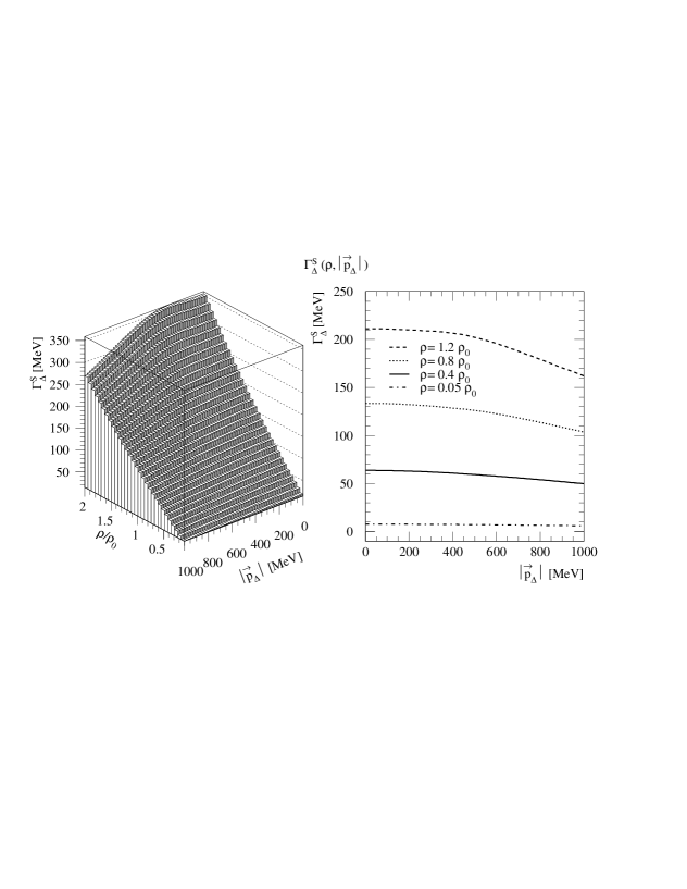
FIG. 3.: (a) In the left panel the spreading width is depicted as a function of the density $\rho$ (in units of the equilibrium density ${\rho}_{0}$ [$k_{F}^{0}=1.333fm^{-1}$]) and the $\Delta$ 3-momentum $|{\vec{p}}_{\Delta}|$ at $W_{\Delta}=1232$ MeV calculated in the Fermi-gas model. (b) The right panel shows the results for this calculation in function of the $\Delta$ 3-momentum $|{\vec{p}}_{\Delta}|$ for the 4 different densities stated in the figure.

FIG. 4.: The effective nucleon mass $M_{N}^{\star}$ as a function of the density $\rho$ (in units of the equilibrium density ${\rho}_{0}$ (value depending on the model)) for the mean-field calculations I and II as explained in section II D.

FIG. 5.: The Pauli-corrected decay width $\Gamma_{\Delta}^{D}$ and the spreading width $\Gamma_{\Delta}^{S}$ as a function of the $\Delta$ 3-momentum $|{\vec{p}}_{\Delta}|$ calculated in the $\sigma\omega-$model at $W^{\star}_{\Delta}=M_{\Delta}^{\star}(\rho)$ for 4 different densities and for the two mean-field calculations as explained in the text.

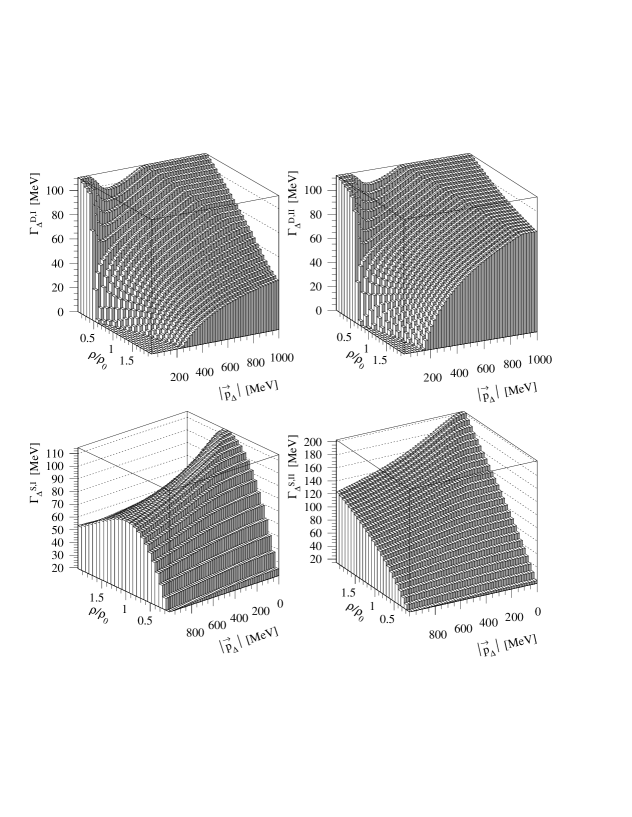
FIG. 6.: The Pauli-corrected $\Delta$ decay width $\Gamma^{D}_{\Delta}$ and the spreading width $\Gamma^{S}_{\Delta}$ in function of the density $\rho$ (in units of the equilibrium density ${\rho}_{0}$ (value depending on the model)) and the $\Delta$ 3-momentum $|{\vec{p}}_{\Delta}|$ calculated in the mean-field model I and II (marked by index I and II respectively) at $W^{\star}_{\Delta}=M_{\Delta}^{\star}(\rho)$.

FIG. 7.: The calculated cross section for Compton scattering off the proton as a function of angle at fixed photon energy, and as a function of photon energy at fixed angle. Data are taken from [31].

FIG. 8.: Differential cross section and photon asymmetry for Compton scattering off ⁴He at an energy of 206 MeV as a function of angle and at an angle of 37^o as a function of energy. The curves represent the results of the Local Density Approximation calculation (LDA) and those for different densities (in units of saturation density) for the mean-field calculation I. Data are taken from [3, 36].

FIG. 9.: Values of the parameters which define the self-energy of the $\Delta$ resonance evaluated at the $\Delta$ invariant mass ($W_{\Delta}$) and three momentum ($|\vec{p}_{\Delta}|$) appropriate for Compton scattering off ⁴He as shown in Fig. (8).

FIG. 10.: LDA calculation of coherent Compton scattering off ⁴He in the Fermi-gas model and the mean-field models I and II. The data are from ref. [3, 36].

FIG. 11.: LDA calculation of coherent Compton scattering off ¹²C in the Fermi-gas model and the mean-field models I and II. The data are from ref. [37].

REFERENCES

- [1] M.-Th. Hütt, A. I. L’vov, A. I. Milstein and M. Schumacher, Phys. Rep. 323, 457 (2000).
- [2] E. Hayward and B. Ziegler, Nucl. Phys. A414, 333 (1984).
- [3] A. Kraus, O. Selke, F. Wissmann et al., Phys. Lett. B 432, 45 (1998).
- [4] B. Körfgen, F. Osterfeld and T. Udagawa, Phys. Rev. C 50, 1637 (1994).
- [5] B. Pasquini and S. Boffi, Nucl. Phys. A598, 485 (1996).
- [6] J. H. Koch and E. J. Moniz, Phys. Rev. C 27, 751 (1983).
- [7] J. H. Koch, E. J. Moniz and N. Ohtsuka, Ann. Phys. (N.Y.) 154, 99 (1984).
- [8] O. Scholten, A. Yu. Korchin, V. Pascalutsa and D. Van Neck, Phys. Lett. B 384, 13 (1996).
- [9] A. Yu. Korchin, O. Scholten and R. Timmermans, Phys. Lett. B 438, 1 (1998).
- [10] L. Tiator, A. K. Rej and D. Drechsel, Nucl. Phys. A333, 343 (1980).
- [11] R. A. Eramzhyan, M. Gmitro and S. S. Kamalov, Phys. Rev. C 41, 2865 (1990).
- [12] D. Drechsel, L. Tiator, S.S. Kamalov and Shin Nan Yang, Nucl. Phys. A660, 423 (1999), nucl-th/9906019.
- [13] R. H. Landau, S. C. Phatak and F. Tabakin, Ann. Phys. (N.Y.) 78, 299 (1973).
- [14] T. Herbert, K. Wehrberger and F. Beck, Nucl. Phys. A541, 699 (1992).
- [15] H. Kim, S. Schramm and S.H. Lee, Phys. Rev. C 56, 1582 (1997).
- [16] L. Liu, X. Luo, Q. Zhou, W. Chen and M. Nakano, Phys. Rev. C 51, 3421 (1995).
- [17] J. D. Walecka, Ann. Phys. (N.Y.) 83, 491 (1974).
- [18] J.D. Bjorken and S.D. Drell, Relativistic Quantum Mechanics (McGraw-Hill,New York, 1964)
- [19] W. Rarita and J. Schwinger, Phys. Rev. 60, 61 (1941).
- [20] M. Benmerrouche, R.M. Davidson and N.C. Mukhopadhyay, Phys. Rev. C 39, 2339 (1989).
- [21] L.M. Nath and B.K. Bhattacharyya, Z. Phys. C 5, 9 (1980).
- [22] M.G. Olsson and E.T. Osypowski, Nucl. Phys. B87, 399 (1975).
- [23] B.D. Serot and J.D Walecka, Adv. Nucl. Phys. 16, 1 (1986).
- [24] T. Suzuki and H. Sakai, Phys. Lett. B 455, 25 (1999).
- [25] F. Gross and W. Surya, Phys. Rev. C 47, 703 (1993).
- [26] M. L. Goldberger and K. M. Watson, Collision Theory (John Wiley and Sons, Inc., 1964).
- [27] R. H. Landau and A. W. Thomas, Phys. Lett. B 61, 361 (1976).
- [28] H De Vries, C. W. De Jager and C. De Vries, Atomic Data and Nuclear Data Tables 36, 495 (1987).
- [29] C. Itzykson and J. -B. Zuber, Quantum Field Theory ( McGraw-Hill Book Company, 1980), p.705.
- [30] V. Pascalutsa, Phys. Lett. B 503, 85 (2001).
- [31] E.L. Hallin et al., Phys. Rev. C 48, 1497 (1993).
- [32] J. C. Bergstrom and E. L Hallin, Phys. Rev. C 48, 1508 (1993).
- [33] S. Kondratyuk and O. Scholten, Nucl. Phys. A677, 396 (2000); nucl-th/0103006.
- [34] D. Drechsel and A. Russo, Phys. Lett. B 137, 294 (1984).
- [35] M.-Th. Hütt and A.I. Milstein, Phys. Rev. C 57, 305 (1998).
- [36] D.Moricciani et al., Few Body Supp. 9, 349 (1995).
- [37] F. Wissmann et al., Phys. Lett. B 335, 119 (1994).
- [38] H. Kurasawa and T. Suzuki, Nucl. Phys. A445, 685 (1985).
- [39] Liang-gang Liu, Phys. Rev. C 51, 3421 (1995).